2
Defining System Context
2.1 Introduction
It is impossible to create a rigorous system model without a precise and formal delineation of the system’s boundaries. We use the term context to describe a boundary definition that includes both the interactions between the system and its environment and the things in the environment with which the system interacts. Defining the system context early is crucial to the effective management of a system’s life-cycle. Omitting this step is an open invitation to uncoordinated and inefficient development, since there is no verified agreement between developers and sponsors on the scope of what is to be built.
Context definition must be done carefully in order to ensure its usefulness. We consider both the context schema, which will be described in this chapter, and its associated lower-level details as parts of the essential (implementation-independent) system model. Therefore, we need to explore how implementation independence will affect our view of the system in its environment. Furthermore, since some consideration of the system’s context must precede any investigation of its function, a context definition should be constructed as an aid in furthering the modeling process.
2.2 Notation for Context Definition
The notation for representing system context is illustrated in Figure 2.1. The context schema uses an extension of the transformation schema notation; each box represents a terminator – something outside the system boundary with which the system interacts – and the transformation, flow, and store symbols are defined as in the transformation schema illustrated in Chapter 6 of Volume 1. The context schema is governed by a number of conventions:
![]() First, only one transformation representing the entire activity of the system appears on the context diagram.
First, only one transformation representing the entire activity of the system appears on the context diagram.
![]() Second, only flows that cross the system boundary may appear on the diagram; flows internal to the system are not shown.
Second, only flows that cross the system boundary may appear on the diagram; flows internal to the system are not shown.
![]() Third, single terminators are used to represent sets of things with which a system interacts. For instance, the terminator Bottle-Filling Valve on the context schema for the Bottling System (Appendix B) represents the set of individual valves with which the system deals.
Third, single terminators are used to represent sets of things with which a system interacts. For instance, the terminator Bottle-Filling Valve on the context schema for the Bottling System (Appendix B) represents the set of individual valves with which the system deals.
![]() Fourth, the store symbol represents stored data shared between the system and a terminator (for example, data about the configuration of the plant, or data to be used in computations). Modification of the stored data by a terminator does not affect the system; likewise, if the system modifies the stored data, the terminators are not affected. The system must be active with respect to the store to obtain input.
Fourth, the store symbol represents stored data shared between the system and a terminator (for example, data about the configuration of the plant, or data to be used in computations). Modification of the stored data by a terminator does not affect the system; likewise, if the system modifies the stored data, the terminators are not affected. The system must be active with respect to the store to obtain input.
![]() Finally, except for flows from a store, the direction of a flow indicates the direction of causality. Output flows are produced by the system, and it is the terminator’s responsibility to handle the flows when they arrive. Similarly, input flows to the system are caused by terminators, and it is the system’s responsibility to decide what to do when they arrive.
Finally, except for flows from a store, the direction of a flow indicates the direction of causality. Output flows are produced by the system, and it is the terminator’s responsibility to handle the flows when they arrive. Similarly, input flows to the system are caused by terminators, and it is the system’s responsibility to decide what to do when they arrive.
Although a flow from a terminator may be prompted by the system, the production of the desired flow is still the responsibility of the terminator. When, and if, the flow finally arrives from the terminator, the system must then respond to it. Note that the idea of causality refers to the responsibility for producing the flow, not to the implementation mechanism for acquiring it. An input flow means the system must accept the flow when it is “there,” even if a read is required to obtain it.
Figure 2.1 Context Schema Notation.

2.3 Context Definition in a Systems Engineering Environment
When a complex system is developed, all the subsystems often evolve together. In the case of a surveillance system, for example, it may be necessary to proceed with development of the embedded computer system that does the data analysis before a final decision has been made about the nature of the sensors that will capture the data. This parallel development situation presents a problem in context definition. The precise nature of the interface to the embedded system may simply not be known at development time.
The extent of this problem may be illustrated by detailing some of the complications that may occur in developing even a simple system. Consider the Cruise Control System (Appendix A). In order to function successfully, the system must perceive the motion of the automobile relative to the Earth. There are a number of ways it could do this. An inertial guidance system is costly and quite exotic by automotive standards, but it would clearly do the job. The guidance system produces a signal proportional to the acceleration of the car. The speed is the time integral of the acceleration, and thus a zero output indicates a constant speed. More realistically, the system might perceive the rotation rate of the wheels by observing the rotation of some mechanical component linked to the wheels. A feasible mechanism for doing this is to attach a magnet to the drive shaft, and to surround the shaft with another magnet. The relative motion of the magnets as the shaft rotates will produce an alternating electric current whose frequency is proportional to the rotation rate. Another feasible mechanism is a mirror affixed to the speedometer cable. If a source of light is aimed at the cable, the mirror will produce a reflected beam once per rotation that can be aimed at a photodetector. The photodetector in turn produces an electrical pulse each time it is illuminated. Although both the magnet and the mirror detection mechanisms produce an alternating electric current, the frequency corresponding to a given speed might be quite different in the two cases.
Let’s now follow the sensor output as it finds its way to the embedded computer system that will use the data to keep the automobile at a constant speed. Assuming the Cruise Control System will utilize a digital processor, the inertial guidance system output would have to be digitized by an analog-digital converter before it could be used; the converter would most likely be connected to the processor by a parallel interface. The inputs of the other two sensors could (after suitable alteration or amplification) be fed into a serial input line of the processor. Alternatively, the signal could drive a pulse counter, which when triggered would provide its current count to the processor across a parallel or serial interface.
Pity the developer of the embedded system when faced with this type of uncertainty! The input signals:
![]() may represent either rotation rate or acceleration,
may represent either rotation rate or acceleration,
![]() may be input in parallel or serial mode, and
may be input in parallel or serial mode, and
![]() may arrive in the form of individual pulses, pulse or digitized translations of analog signals.
may arrive in the form of individual pulses, pulse or digitized translations of analog signals.
As we will demonstrate in the following section, uncertainties of this kind need not preclude a rigorous definition of system boundaries, provided that the concept of implementation-dependence is properly exploited. There are two major guidelines that will assist in creating a context diagram that usefully describes the essence of a system. First, the terminators and flows should be identified from the point of view of the subject matter of the system. Second, the transformation that represents the system should be considered to exclude the interface technology.
2.4 Identification of Terminators and Flows
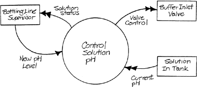
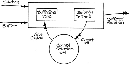
In order to examine terminator and flow identification, let’s use the Bottle-Filling System (Appendix B) as an illustration. The purpose of the embedded system modeled in Figure 2.2 is to control part of the operation by maintaining the solution that is put in the bottles at the proper pH. The subject matter of this system is chemical engineering. However, the flows and terminators have names drawn mainly from computer technology and give a reader no help in understanding the fundamental nature of the system. In Figure 2.3, the problem has been corrected by renaming the flows and terminators with chemical engineering terminology.
Figure 2.2 Context Schema with Poorly Chosen Names.

It is instructive to reexamine Figures 2.2 and 2.3 considering the terminology described in Chapter 1, that is, in terms of the perception/action space, sensors/actors, communication links, and processors. Figure 2.2 shows the embedded system’s interaction with the communications links. Figure 2.3, on the other hand, describes interaction with things in the system’s perception/action space, such as the solution, and with sensors/actors, such as the buffer inlet valve; the supervisor could be in either category. Thus, saying that the description of the system’s environment has moved away from the immediate surroundings of the system and toward the perception/action space, and saying that the terminology has become more subject-matter-oriented, reflects two views of the same phenomenon. Showing the system input as Current pH rather than as Digital Input permits rigorous definition of input characteristics (for example, range and required precision of measurement), while deferring issues such as serial versus parallel to the implementation model.
Figure 2.3 Context Schema with Well-Chosen Names.
Let’s return to the observation that in Figure 2.3 the decision has been made to retain (in the case of the buffer inlet valve) some details of the actor technology. It would have been possible as an alternative to show an output called Required pH Change from the system to the Solution terminator. However, the system context seems easier to visualize from Figure 2.3 as shown. Here are some rough guidelines for making such choices. Show the sensor/actor technology when:
![]() the sensor/actor technology has been defined in detail;
the sensor/actor technology has been defined in detail;
![]() the sensor/actor technology is more closely related to the subject matter of the system than to the technology of computer peripheral devices;
the sensor/actor technology is more closely related to the subject matter of the system than to the technology of computer peripheral devices;
![]() a sensor must be controlled by the embedded system in order to perform its function (for example, a movable optical detector); and/or
a sensor must be controlled by the embedded system in order to perform its function (for example, a movable optical detector); and/or
![]() the nature of the data received from or sent to the environment is fundamentally dependent on the choice of sensor or actor.
the nature of the data received from or sent to the environment is fundamentally dependent on the choice of sensor or actor.
Show the objects in the system’s perception/action space when:
![]() the sensor/actor technology is not well-defined;
the sensor/actor technology is not well-defined;
![]() the sensor/actor technology is not closely related to the subject matter of the system (for example, general purpose I/O peripherals);
the sensor/actor technology is not closely related to the subject matter of the system (for example, general purpose I/O peripherals);
![]() a sensor passively sends through data about the perception space to the embedded system;
a sensor passively sends through data about the perception space to the embedded system;
![]() the nature of the data sent to or received from the environment is relatively independent of sensor/actor technology; and/or
the nature of the data sent to or received from the environment is relatively independent of sensor/actor technology; and/or
![]() the interface between the system and a human operator is being described.
the interface between the system and a human operator is being described.
The basic principle is to show the sensor/actor technology only when it is likely to be visible to the software or hardware carrying out the application-specific work of the system.
Let’s now look at the second guideline for creating the context schema.
2.5 Exclusion of Interface Technology
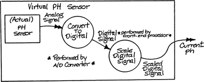
It may seem superfluous to say that the transformation represented on the context schema contains no interface implementation details, since no details of the transformation are shown in any case. However, we want to show that the modeler’s picture of how the interface technology relates to the context schema can affect the way the diagram is built. Consider again the relationship between Figures 2.2 and 2.3. It is tempting to think that in moving to Figure 2.3 we have incorporated the display terminal and the converters into our view of the system. A better way to visualize the situation – suggested by Figure 2.4 – is that interface technology surrounds the context diagram, separating the real actors, sensors, and perception/action space objects from the virtual actors, sensors, and objects perceived by the system. (This idea is closely related to the idea of a virtual device as advocated by Britton, Parker, and Parnas [1]). A specific instance of this placement of implementation technology is shown in Figure 2.5, which shows details of the current pH input from the solution terminator in Figure 2.3. This shows the sequence of transformations necessary to connect a portion of the real environment of the pH control system to its virtual environment. The box surrounding the implementation technology may be thought of as the “virtual pH sensor.”
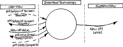
As another illustration, this time from the point of view of a human interface, we may return to Figure 2.3 and focus on the input labeled New pH Level. Now consider the actual procedure that a supervisor sitting at a video display terminal might carry out to enter a new setpoint:
(1) Hit a control key that causes display of a setpoint screen. This screen shows the current setpoint and permits overwriting it.
(2) Overwrite all or part of the current setpoint to specify a new value.
(3) Receive an error message describing any errors made such as an out-of-range value entered.
(4) Correct any errors and hit a control key indicating that the data is complete.
Figure 2.4 Visualization of Implementation Technology.
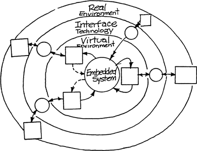
Figure 2.5 Implementation Technology Detail.
Notice that the user’s view of the data entry procedure is quite different from the system’s view (Figure 2.6) – the system’s view is implementation-independent; the user’s view is dependent on the implementation technology of user-system interface. For this reason, modeling the user view of the system interface is deferred to the implementation model.
Figure 2.6 User and System Views of Data Entry.
As with the identification conventions described in the last section, excluding interface details allows a precise description of system boundaries. The effect of this exclusion is a prescription of the required interface between the essential system and the world outside. The implementer is then free to choose sensors, actors, and communication links at will as long as the essential interface characteristics are preserved.
2.6 Expanded Contexts – Material and Energy Transformations
In all the examples given so far in this chapter, the terminators have been communication links, sensors/actors, or objects in the perception/action space of the system. Correspondingly, the flows have represented data or control messages between the embedded system and the terminators. We have shown that in such cases, the concept of a virtual environment for the embedded system allows development to proceed in the absence of final decisions about sensor/actor technology.
Let’s now consider a different strategy. Suppose that the overall system includes transformations of material or of energy from one form to another. Suppose also that either the nature of the sensors and actors that will perform these transformations, or the details of the interface between the sensors/actors and the embedded system, are unknown. Figure 2.7 illustrates a context schema for the Bottle-Filling System (Appendix B) that would be appropriate in such a situation. The characteristics of this context schema are:
![]() The material/energy flows depict the objects that enter and leave the perception/action space of the system.
The material/energy flows depict the objects that enter and leave the perception/action space of the system.
![]() The terminators that send and receive the material and energy flows are outside the perception/action space.
The terminators that send and receive the material and energy flows are outside the perception/action space.
![]() The material and energy transformations are visualized as being inside the transformation that represents the system boundary.
The material and energy transformations are visualized as being inside the transformation that represents the system boundary.
Figure 2.7 An Expanded Context Schema.

Modeling a system in this way is often helpful in understanding data transformation requirements in a system such as a manufacturing plant, where the structure of the data and control transformations is determined by the nature of the production process. It is vital to understand the flow of material/energy in such a system, where the complexity of the manufacturing process is a barrier to an integrated view of the plant. The specification for systems of this kind is ultimately dependent on the physics, chemistry, or biology of the underlying processes.
However, the context of the embedded system must ultimately be defined for detailed development to occur. In order to carry out this “context reduction,” the individual material and energy transformations must first be modeled, as illustrated by Figure 2.8. Each material or energy transformation contained within the expanded context must be reconstructed to show the objects or sensors and actors in the real world, and the embedded system with which they interact. This reconstruction is necessarily based on the technology used to carry out the material/energy transformation. The terminators shown on the resulting context schema incorporate the material transformation. This can be visualized as shown in Figure 2.9. Notice that the physical material (the solution) is now completely excluded from the embedded system, having been removed to the terminator.
Figure 2.8 Portion of Model Built from Expanded Context Schema.

Figure 2.9 Reduction of Context to Exclude Material Transformations.
2.7 Defining Context Specifics
The context schema provides a definition of the boundary between a system and its environment, but it provides few details. As with the other schemas we have discussed, the specifics for the components declared on the schema must be defined. The context schema is also the highest level in the leveled model, and therefore the details of the context schema are redundant with the details of the behavioral model. However, it is helpful to begin some definition at the time we construct the context schema.
Flows and stores on the context schema play the same role as they do on the transformation schema. They have meaning, composition, and type as described in Volume 1, Chapter 11, (Specifying Data). At context definition time, however, typically only the meaning is well-understood. Composition or type definitions are often not available, in which case they must be delayed until the detailed construction of the behavioral model. The meanings of flows and stores on the context schema should be specified as a part of context definition (and, if known, so should the composition or type). Failure to define the meanings of flows and stores will make review and verification of the context schema impossible.
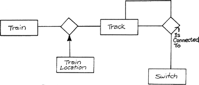
The terminators that appear on the context schema represent objects or sensors/actors in the system’s environment with which the system interacts. Since these entities are in the system’s perception/action space, the system will often need to store data about them and about their interactions. Interactions between terminators may be either active or passive. An active interaction is represented by an external event that occurs in a terminator (or terminators) and causes the system to make a response that affects the activities of other terminators. For example, Figure 2.10 shows a portion of a train control system context schema. As the trains move on the tracks, the locations of the trains are updated. Depending on the locations of other trains, the trains may be commanded to speed up or slow down as appropriate. There is thus an active interaction between the Track terminator and the Train terminator. A passive interaction exists between the Switch and the Track terminators. The location of the switches with respect to the tracks must be stored by the system so that trains may be effectively switched from track to track.
Figure 2.10 Train Control Context Schema.

The data schema, with its associated specifics, is an appropriate tool for modeling terminators and their active and passive interactions. A preliminary data schema such as the one illustrated in Figure 2.11 may be a useful adjunct to the context schema.
Figure 2.11 Train Control Preliminary Data Schema.
The precise behavior of the transformation on the context schema is to be described by the behavioral model. However, to aid in the construction of the behavioral model, we need to know the purpose or objective of the system. A short narrative text description of this purpose should be added to the context schema. The document should focus only a high-level description of the intent of the system; it should not be a description of the functional requirements – that is properly left to the behavioral model.
Finally, a description of the desired attributes of the system should also be added to the model. An attribute of a system is a characteristic of the system as a whole. For example, availability or reliability attributes, mean-time-between-failure, mean-time-to-repair, and the like describe the overall characteristics of the system in operation. Growth needs of the system, its lifetime, and maintainability characteristics also properly qualify as attributes of the system. Again, this description should not encroach on the responsibilities of the behavioral model.
Context schemas can easily become quite large, even unmanageable. To solve this problem with the transformation schema, we leveled the model to reduce complexity as described in Chapter 12 of Volume 1 (Organizing the Model). In the next two sections, we shall discuss some issues in the construction of large context schemas.
2.8 Packaging Context Flows
Packaging of flows is a strategy for reducing the complexity of a context schema. The fundamental guideline for packaging, as with the transformation schema, is that the internal organization of a flow should match the meaning of the flow to the system.
As an example, consider Figure 2.12, which shows several packaged flows. Tank Levels is not a helpful packaging; the system is likely to respond differently to an empty supply tank than to an empty reaction tank. (A corresponding packaging of the terminators would also suppress useful information since the tanks play different roles for the system.) On the other hand, Reaction Tank Status could also be a packaged flow (containing level and fill rate, for example), but it represents a single cohesive unit for the receiver.
Figure 2.12 Context Schema with Poorly Packaged Flows.

Flows should be packaged when the packaged flow forms a cohesive unit of interest to the receiver.
Flows should not be packaged when:
![]() the flows occur asynchronously;
the flows occur asynchronously;
![]() the flows require a “tag” (identifier) to separate out the components on receipt; or
the flows require a “tag” (identifier) to separate out the components on receipt; or
![]() the flows come from separate terminators.
the flows come from separate terminators.
2.9 Leveled and Multiple-Context Schemas
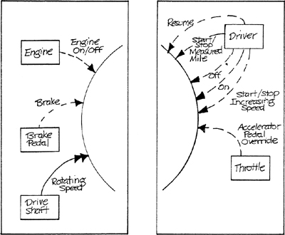
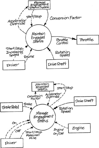
Even if flows are packaged, the context schema is often still too large for a single screen. The solution is simple: split the diagram onto several screens. An example is shown in Figure 2.13. The several screens together make up a complete context schema. We describe the set as a leveled context schema.
Figure 2.13 A Simple Leveled Context Schema.
An alternative approach, which is particularly useful when a development project is split into several independent teams, is to draw multiple context schemas, as illustrated in Figure 2.14. In this approach, the schemas show their connections by drawing the companion system as a terminator. Each subsystem can then be developed independently.
2.10 Summary
Context definition is a first step in defining the scope of the system; without such a definition development is difficult, if not impossible. We have introduced a notation for defining system scope and provided some heuristics for constructing the definition. Most importantly, heuristics have been provided for context construction in ill-defined environments.
Figure 2.14 Multiple Context Schemas.
Chapter 2: References
1. K.H. Britton, R.A. Parker, and D.L. Parnas. A Procedure for Designing Abstract Interfaces for Device Interface Models. Proceedings, Fifth International Conference on Software Engineering, IEEE, 1981, pp. 195-204.