Computational Methods for Derivatives with Early Exercise Features
Carl Chiarellaa, Boda Kangb, Gunter Meyerc and Andrew Ziogasd, aFinance Discipline Group, UTS Business School, University of Technology, Sydney, Australia, bDepartment of Mathematics, University of York, Heslington, York, UK, cDepartment of Mathematics, Georgia Institute of Technology, Atlanta, GA, USA, dLloyds Bank – Commercial Banking, Sydney, Australia
Abstract
In this paper we consider various computational methods for pricing American style derivatives. We do so under both jump diffusion and stochastic volatility processes. We consider integral transform methods, the method of lines, operator-splitting, and the Crank-Nicolson scheme, the latter being used to generate the benchmark solution. Overall, we find that the method of lines approach is quite competitive with other methods for the problems considered in this paper. As one goes to higher dimensions it may be necessary to use methods such as the sparse grid approach.
Keywords
American option pricing; Stochastic volatility; Jump dynamics; Fourier transforms; Crank-Nicolson scheme
JEL Classification Codes
G3; C02
1 General Introduction
The American option pricing problem has been explored in great depth in the option pricing literature. The survey by Barone-Adesi (2005) provides an overview of this research for the case of the American put under the classical Brownian motion process for asset returns.
An array of approaches have been proposed in the vast literature on this topic. It will not be possible in this paper to survey all of these. Rather we shall focus on the methods that the authors and their co-workers have found to be the most useful. In particular we shall focus first on the formulation of the problem. In order to capture the market reality that the underlying asset returns are not well modeled by Brownian motion, it is necessary to consider both stochastic volatility and jump-diffusion dynamics as these are the processes most widely used to capture these effects. More recently there has been a great deal of work on the use of Lévy processes, which is nicely surveyed in the book by Cont and Tankov (2003). Space limitations do not allow us to go into all of these approaches here.
In particular in this paper we shall survey the integral transform approach, which in higher dimensions can only work for specific correlation structures, and the partial differential equation approach. For the latter we shall propose a number of finite difference approaches, projected successive over-relaxation (PSOR), which when used with a high level of discretization will yield a benchmark solution against which we can compare other methods, the method of lines (MOL) which the authors have found applies quite successfully to low dimensional problems, and sparse grid and operator-splitting methods for higher dimensional problems.
The paper is structured as follows. In Section 2 we shall give a formulation of the American option pricing problem, first of all in the case of geometric Brownian motion and then, for more general dynamics, for the underlying asset price that allows both stochastic volatility and poisson jump dynamics. Section 3 will introduce the integral transform approach, first in one dimension and then in several dimensions. Section 4 will introduce the method of lines (MOL) for the situation when the underlying asset is driven by both stochastic volatility and Poisson jump dynamics. The performance of the MOL approach is compared against the operator-splitting approaches, in particular the componentwise splitting method and the finite difference method with PSOR, both of which are discussed in Section 4 as well. Section 5 will conclude.
2 The Problem Statement—In the Case of Stochastic Volatility and Poisson Jump Dynamics
Let ![]() be the price of an American call option written on a stock of price
be the price of an American call option written on a stock of price ![]() with time to expiry
with time to expiry ![]() 1and strike price
1and strike price ![]() . For the underlying dynamics, we assume that the stochastic differential equation (SDE) for
. For the underlying dynamics, we assume that the stochastic differential equation (SDE) for ![]() is given by the jump-diffusion process proposed by Merton (1976), in conjunction with the square root variance process of Heston (1993). Thus the dynamics for
is given by the jump-diffusion process proposed by Merton (1976), in conjunction with the square root variance process of Heston (1993). Thus the dynamics for ![]() under the so-called historical measure
under the so-called historical measure ![]() are governed by the SDE system
are governed by the SDE system
![]() (1)
(1)
![]() (2)
(2)
In (1), ![]() is the instantaneous stock return per unit time,
is the instantaneous stock return per unit time, ![]() is the instantaneous squared stock variance per unit time, and
is the instantaneous squared stock variance per unit time, and ![]() is a standard Wiener process under
is a standard Wiener process under ![]() . Furthermore, we define the Poisson jump arrival process
. Furthermore, we define the Poisson jump arrival process ![]() by
by

and set
![]() (3)
(3)
where ![]() is the continuous probability density function for the multiplicative jump sizes,
is the continuous probability density function for the multiplicative jump sizes, ![]() , generated by the measure
, generated by the measure ![]() . In (2),
. In (2), ![]() is the long-run mean for
is the long-run mean for ![]() is the rate of mean reversion,
is the rate of mean reversion, ![]() is the instantaneous volatility of
is the instantaneous volatility of ![]() per unit time (the so-called vol-of-vol), and
per unit time (the so-called vol-of-vol), and ![]() is a standard Wiener process under
is a standard Wiener process under ![]() correlated with
correlated with ![]() such that
such that ![]() . Note that
. Note that ![]() ,
, ![]() , and
, and ![]() are otherwise uncorrelated.
are otherwise uncorrelated.
Let ![]() (assumed constant) be the risk-free rate of interest, and assume that the stock pays a continuously compounded dividend yield at the rate
(assumed constant) be the risk-free rate of interest, and assume that the stock pays a continuously compounded dividend yield at the rate ![]() (also assumed constant). We assume, following Heston (1993), that the market price of variance risk is proportional to
(also assumed constant). We assume, following Heston (1993), that the market price of variance risk is proportional to ![]() , and is of the form
, and is of the form ![]() , where
, where ![]() is a constant. Using standard hedging arguments and an application of Ito’s lemma for jump-diffusion processes, it can be shown2 that
is a constant. Using standard hedging arguments and an application of Ito’s lemma for jump-diffusion processes, it can be shown2 that ![]() satisfies the partial integro-differential equation (PIDE)
satisfies the partial integro-differential equation (PIDE)
 (4)
(4)
in the region ![]() , and
, and ![]() . Here
. Here ![]() denotes the early exercise boundary at time to maturity
denotes the early exercise boundary at time to maturity ![]() and variance level
and variance level ![]() , and
, and ![]() denotes the market price of risk associated with a jump in the value of the stock with magnitude
denotes the market price of risk associated with a jump in the value of the stock with magnitude ![]() (that is a jump from
(that is a jump from ![]() to
to ![]() ). The initial condition for (4) is the American call payoff function, given by
). The initial condition for (4) is the American call payoff function, given by
![]() (5)
(5)
The boundary condition at ![]() is less obvious. Some authors (such as Clarke and Parrott (1999), and Ikonen and Toivanen (2007)) prefer to use the exercise payoff condition
is less obvious. Some authors (such as Clarke and Parrott (1999), and Ikonen and Toivanen (2007)) prefer to use the exercise payoff condition ![]() . Alternatively we note that by setting
. Alternatively we note that by setting ![]() in (4) we find that
in (4) we find that ![]() is given by the solution of the PIDE
is given by the solution of the PIDE
 (6)
(6)
We have preferred to let the model itself yield the boundary condition by extrapolating the solution for ![]() to
to ![]() as detailed in Section 4.1. This procedure is justified by the fact that the boundary condition at
as detailed in Section 4.1. This procedure is justified by the fact that the boundary condition at ![]() is an outflow condition as demonstrated in Chiarella et al. (2009). Also we have found that it yields the same solution as solving (6) but is computationally more efficient to implement.
is an outflow condition as demonstrated in Chiarella et al. (2009). Also we have found that it yields the same solution as solving (6) but is computationally more efficient to implement.
Since, in the limit as ![]() the option price becomes insensitive to the variance we have
the option price becomes insensitive to the variance we have
![]() (7)
(7)
In the asset domain, the boundary conditions are
![]() (8)
(8)
![]() (9)
(9)
Condition (8) is the trivial condition that the option is worthless when the stock price falls to zero. Condition (9) follows because the option value is equal to the payoff at the free boundary and is known as the value-matching condition. Finally we require two additional conditions along the early exercise surface, namely
![]() (10)
(10)
The boundary conditions (10) are referred to in the literature as the smooth-pasting conditions, and follow by assuming the elimination of arbitrage opportunities. Mathematically, this is equivalent to ensuring that ![]() and
and ![]() will be continuous for all values of
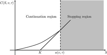
will be continuous for all values of ![]() . Figure 1 demonstrates the payoff, price profile, and early exercise boundary for the American call under consideration.
. Figure 1 demonstrates the payoff, price profile, and early exercise boundary for the American call under consideration.
The PIDE (4) may be written in the form
 (11)
(11)
![]() (12)
(12)
and
![]() (13)
(13)
with ![]() and
and ![]() , and we note that
, and we note that
![]()
where ![]() is a density function under the risk-neutral pricing measure
is a density function under the risk-neutral pricing measure ![]() . The relevant boundary conditions are (5–9), and the domain for the problem is
. The relevant boundary conditions are (5–9), and the domain for the problem is ![]() , and
, and ![]() .
.
Option pricing under stochastic volatility and jump-diffusion dynamics of course involves market incompleteness since both the variance risk and the jump risk are not priced in the market. When the market is incomplete option pricing formulae are not unique. In (11) the non-uniqueness is reflected in the market price of variance risk parameter ![]() (embedded in the parameter
(embedded in the parameter ![]() ) and the market price of jump risk
) and the market price of jump risk ![]() that is embedded in the parameter
that is embedded in the parameter ![]() and jump-size distribution under the adjusted measure
and jump-size distribution under the adjusted measure ![]() (see Eq. (12)). There is a large literature on how these parameters may be chosen, for instance, by minimizing the variance of hedging cost or some entropy measure. Here we shall simply assume that the parameters
(see Eq. (12)). There is a large literature on how these parameters may be chosen, for instance, by minimizing the variance of hedging cost or some entropy measure. Here we shall simply assume that the parameters ![]() as well as the parameters of the distribution
as well as the parameters of the distribution ![]() have somehow been obtained either by the methods referred to or simply by calibration to market data.
have somehow been obtained either by the methods referred to or simply by calibration to market data.
Our main task in Sections 3 and 4 is to develop approaches to solving the PIDE (11) subject to the boundary conditions (5–10). In later sections we shall consider some higher dimensional problems. As we indicated in the Introduction we shall survey both the integral transform approach and the discretisation of the PIDE. The main numerical challenges in solving (11) arise from (i) the two spatial dimensions (![]() and
and ![]() ) so that we are seeking an early exercise surface, and (ii) the integral term over the jump-size distribution which will involve the unknown option price over a whole set of values of
) so that we are seeking an early exercise surface, and (ii) the integral term over the jump-size distribution which will involve the unknown option price over a whole set of values of ![]() .
.
3 American Call Options Under Jump-Diffusion Processes
In this section we shall drop the stochastic volatility component from the dynamics by assuming that the variance is constant and merely discuss how to handle the jump term in the integral transform approach. Option pricing under jump-diffusion dynamics was originally investigated by Merton (1976) for the case of the European option.
3.1 Introduction
The integral transform technique can be applied to solving the option pricing problem under a range of underlying dynamics and payoff types. There are numerous examples where integral transforms have been used in the option pricing literature. Scott (1997) uses Fourier transforms to value European options under jump-diffusion with both stochastic volatility and stochastic interest rates. Carr and Madan (1999) with a particular focus on the variance gamma model use Fourier transforms to motivate numerical algorithms using the fast Fourier transform. The American strangle has been analyzed by Chiarella and Ziogas (2005) using a Fourier transform approach, under the assumption that the underlying dynamics are the classic geometric Brownian motion.
The main advantage of the Fourier transform method is that the solution may be expressed in terms of a general initial value or payoff function, so that a wider variety of American options, such as puts, calls, butterflies, spread options, and max-options can all be handled systematically.
In this section we derive the linked system of integral equations for the price and early exercise boundary of an American call under Merton’s jump-diffusion dynamics. We also derive the limit of the early exercise boundary at maturity, and discuss a numerical algorithm for solving the linked integral equation system. We do so by extending to the jump-diffusion situation the quadrature integration technique of Kallast and Kivinukk (2003). The algorithm used has the added advantage of generating values for the price, delta, and early exercise boundary. The issue of the existence and uniqueness of the solution to the nonlinear integral equation that arises in the solution of the free boundary value problem was raised by Myneni (1992) and finally settled by Peskir (2005) in the case of pure diffusion dynamics. It still remains to extend that analysis to the case of jump-diffusion dynamics.
We focus on deriving solutions to the partial differential equation (PDE) for the American call price. A natural solution technique here is the integral transform approach, which (see Debnath, 1995) has been very successfully employed in a wide range of PDE problems in the natural sciences. One of the difficulties with dealing with American options using this technique arises from the fact that one has to solve the PDE on a region restricted by the early exercise, or free, boundary. McKean (1965), who seems to have been the first to consider the American option pricing problem, solves the homogeneous PDE in a restricted domain by using an incomplete Fourier transform. An alternative approach, developed by Jamshidian (1992), replaces the homogeneous PDE with an equivalent inhomogeneous PDE on an unrestricted domain. The solution to this alternative formulation can then be derived by using the standard Fourier transform, and then through an application of Duhamel’s principle. In this section we provide this extension of Jamshidian’s formulation to the jump-diffusion case.
While some authors, in particular Pham (1997) and Gukhal (2001), derive integral equations for the price and free boundary of American options under jump-diffusion they do not discuss how they can be solved numerically. In this section we solve the linked integral equation system that arises for the American call and its free boundary in the case of jump-diffusion. In developing a numerical scheme for the linked integral equation system we obtain a simplification of the integral terms over the jump-size distribution that reduces the computational burden by reducing the dimension of the multiple integration involved. We give some results on the behavior of the early exercise boundary at expiry that are needed to start the numerical procedure. We use the proposed numerical integration scheme to find the price, delta, and early exercise boundary of American calls with log-normal jump sizes. We also demonstrate that the method is often more efficient than a simple two-pass Crank-Nicolson finite difference scheme and is competitive with the method of lines of Meyer (1998) (alternatively, see Meyer, 2012).
Section 3.2 outlines the free boundary problem that arises from pricing an American call option under Merton’s jump-diffusion model. Section 3.3 applies Jamshidian’s method to derive an inhomogeneous PIDE for the American call price, which is then solved using Fourier transforms. We thus obtain the linked integral equation system for the free boundary and option price. We derive the limit of the free boundary at expiry in Section 3.4, and find that this limit is different from that found for pure diffusion models. Section 3.5 analyzes the integral equations in the case where the jump sizes follow a log-normal distribution, as suggested by Merton (1976). Section 3.7 outlines the numerical integration method used to solve the linked integral equation system for the free boundary, price, and delta of the American call. Since the integral equation for the call value and the integral equation for the free boundary are interdependent, we provide a method to handle this interdependence in order to use the two-pass sequential procedure that works well in the non-jump case. Numerical results detailing the efficiency of this algorithm are provided in Section 3.8. As this section summarizes the paper by Chiarella and Ziogas (2009) we shall refer the reader to that paper for many of the proofs.3
3.2 Problem Statement—Merton’s Model
As we drop the stochastic volatility component of Section 2 we simply write ![]() to denote the price of an American option written on the underlying asset
to denote the price of an American option written on the underlying asset ![]() at time to expiry
at time to expiry ![]() . In this case the free boundary only depends on
. In this case the free boundary only depends on ![]() so we write it as
so we write it as ![]() . Because in this section
. Because in this section ![]() is constant the dynamics for
is constant the dynamics for ![]() follows the jump-diffusion process
follows the jump-diffusion process
![]() (14)
(14)
where in addition to the notation introduced in Section 2 we set the instantaneous variance per unit time as a constant ![]() and
and ![]() is a standard Wiener process under the physical measure.
is a standard Wiener process under the physical measure.
The PIDE (4) for ![]() in the current case becomes4
in the current case becomes4
 (15)
(15)
which has to be solved in the region ![]() and
and ![]() . Given a form for
. Given a form for ![]() , we can define a new intensity,
, we can define a new intensity, ![]() , and jump-size distribution,
, and jump-size distribution, ![]() , which fully incorporate the term
, which fully incorporate the term ![]() , such that (15) can be written as
, such that (15) can be written as
 (16)
(16)
The market incompleteness of the jump-diffusion option pricing problem is reflected in the fact that the choice of ![]() and
and ![]() is at the discretion of the model builder, so that the associated risk-neutral density is non-unique. As stated earlier, we take the view here that the model builder would calibrate
is at the discretion of the model builder, so that the associated risk-neutral density is non-unique. As stated earlier, we take the view here that the model builder would calibrate ![]() and
and ![]() directly to market data without needing to determine a risk-neutral density for the pricing problem at hand. Henceforth, for ease of notation, we shall simply refer to the jump risk-adjusted intensity and jump-size density in (16) as
directly to market data without needing to determine a risk-neutral density for the pricing problem at hand. Henceforth, for ease of notation, we shall simply refer to the jump risk-adjusted intensity and jump-size density in (16) as ![]() and
and ![]() respectively.
respectively.
By use of (3), the PIDE (16) can be written as
 (17)
(17)
In the case of an American call option, the initial and boundary conditions (5, 7–10) become
![]() (18)
(18)
![]() (19)
(19)
![]() (20)
(20)
![]() (21)
(21)
and the PIDE (17) is solved subject to these.5
If we were to use the approach of McKean (1965) we would introduce an incomplete version of the Fourier transform, defined by (note that ![]() , and
, and ![]() )
)
![]() (22)
(22)
Inversion of the transform is readily carried out, and the end result is a linked system of integral equations for ![]() and
and ![]() . This solution method comes at the expense of the drawbacks reported by Chiarella and Ziogas (2009).6
. This solution method comes at the expense of the drawbacks reported by Chiarella and Ziogas (2009).6
We instead seek a more efficient alternative for solving (17–21) using the standard Fourier transform.
3.3 Jamshidian’s Representation
One of the major difficulties in solving the PIDE (17) subject to the boundary conditions (18–21) is that the solution is sought on a restricted domain for the stock price ![]() , and furthermore the boundary of this domain is itself unknown a priori and needs to be determined as part of the solution process. In the pure diffusion case, Jamshidian (1992) demonstrates that by evaluating the PDE for the American call price when
, and furthermore the boundary of this domain is itself unknown a priori and needs to be determined as part of the solution process. In the pure diffusion case, Jamshidian (1992) demonstrates that by evaluating the PDE for the American call price when ![]() , one can reformulate the free boundary problem in the restricted domain
, one can reformulate the free boundary problem in the restricted domain ![]() as an inhomogeneous PDE in the unrestricted domain
as an inhomogeneous PDE in the unrestricted domain ![]() . This inhomogeneous PDE can then be more readily solved by traditional solution techniques such as Fourier transforms. We note that the free boundary value problem (FBVP) given by (17–21) involves a homogeneous PIDE to be solved in the restricted asset price domain
. This inhomogeneous PDE can then be more readily solved by traditional solution techniques such as Fourier transforms. We note that the free boundary value problem (FBVP) given by (17–21) involves a homogeneous PIDE to be solved in the restricted asset price domain ![]() . We shall apply Jamshidian’s approach to reformulate the PIDE (17) and associated boundary conditions as an inhomogeneous PIDE on an unrestricted domain.
. We shall apply Jamshidian’s approach to reformulate the PIDE (17) and associated boundary conditions as an inhomogeneous PIDE on an unrestricted domain.
We highlight the fact that ![]() and
and ![]() are continuous for
are continuous for ![]() and
and ![]() , as given by the value-matching condition (20) and smooth-pasting condition (21). Jamshidian’s approach can only be applied with confidence when such continuity holds. We now state the main result that converts the homogeneous PIDE on a restricted domain to an inhomogeneous PIDE on an unrestricted domain.
, as given by the value-matching condition (20) and smooth-pasting condition (21). Jamshidian’s approach can only be applied with confidence when such continuity holds. We now state the main result that converts the homogeneous PIDE on a restricted domain to an inhomogeneous PIDE on an unrestricted domain.
Gukhal (2001) provides clear economic interpretation for the inhomogeneous term that arises in Eq. (23). The ![]() term represents the net cash flows received from holding the portfolio
term represents the net cash flows received from holding the portfolio ![]() whenever
whenever ![]() is in the stopping region. This is already familiar from the pure diffusion case (see, for example, Kim, 1990). The integral term arises entirely because of the introduction of jumps in the price process for
is in the stopping region. This is already familiar from the pure diffusion case (see, for example, Kim, 1990). The integral term arises entirely because of the introduction of jumps in the price process for ![]() . Note that if no jumps were present (
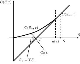
. Note that if no jumps were present (![]() =0) then this term would be zero, and the inhomogeneous term would become the same one presented by Jamshidian (1992). This additional term captures the rebalancing costs incurred by the option holder whenever the price of the underlying jumps down from the stopping region back into the continuation region. Figure 2 illustrates this effect in detail. Consider the case where, during the life of the option contract, the underlying asset price is at
=0) then this term would be zero, and the inhomogeneous term would become the same one presented by Jamshidian (1992). This additional term captures the rebalancing costs incurred by the option holder whenever the price of the underlying jumps down from the stopping region back into the continuation region. Figure 2 illustrates this effect in detail. Consider the case where, during the life of the option contract, the underlying asset price is at ![]() . Since the value of
. Since the value of ![]() is in the stopping region, the holder of the option will currently possess the portfolio
is in the stopping region, the holder of the option will currently possess the portfolio ![]() . If a jump of size
. If a jump of size ![]() occurs such that
occurs such that ![]() , then the portfolio held by the investor will now be worth less than the unexercised American call. This difference is the cost being captured by the integral in the inhomogeneous term in (23).
, then the portfolio held by the investor will now be worth less than the unexercised American call. This difference is the cost being captured by the integral in the inhomogeneous term in (23).
Having derived the inhomogeneous PIDE for ![]() we next use Fourier transforms to find the solution. Our first step is to transform the PIDE to an equation with constant coefficients and a “standardized” strike of 1. Let
we next use Fourier transforms to find the solution. Our first step is to transform the PIDE to an equation with constant coefficients and a “standardized” strike of 1. Let ![]() and
and ![]() , with
, with ![]() . The transformed PIDE for
. The transformed PIDE for ![]() is then
is then
 (25)
(25)
where ![]() . Equation (25) is to be solved in the time domain
. Equation (25) is to be solved in the time domain ![]() , and the unrestricted region
, and the unrestricted region ![]() , subject to the initial and boundary conditions
, subject to the initial and boundary conditions
![]() (26)
(26)
![]() (27)
(27)
![]() (28)
(28)
It is worth noting that the smooth-pasting condition still holds, although we do not explicitly require it when solving (25) for ![]() since it is incorporated in the inhomogeneous term.7
since it is incorporated in the inhomogeneous term.7
Since the ![]() -domain is now the unrestricted region
-domain is now the unrestricted region ![]() , the Fourier transform of the inhomogeneous PIDE (25) can be found. Define the Fourier transform of
, the Fourier transform of the inhomogeneous PIDE (25) can be found. Define the Fourier transform of ![]() , as
, as
![]() (29)
(29)
with the corresponding inversion formula
![]() (30)
(30)
where ![]() is the complex number. Applying this Fourier transform to (25), we can reduce the inhomogeneous PIDE for
is the complex number. Applying this Fourier transform to (25), we can reduce the inhomogeneous PIDE for ![]() to an inhomogeneous ordinary differential equation (ODE) for
to an inhomogeneous ordinary differential equation (ODE) for ![]() , whose solution is readily found.
, whose solution is readily found.
When taking the Fourier transform of (25), we note that ![]() and
and ![]() do not approach zero as
do not approach zero as ![]() . A number of approaches have been suggested for dealing with this difficulty. Carr and Madan (1999) and Lee (2004) suggest introducing a damping function of the form
. A number of approaches have been suggested for dealing with this difficulty. Carr and Madan (1999) and Lee (2004) suggest introducing a damping function of the form ![]() for some positive constant
for some positive constant ![]() , and then apply the transform to the dampened option price
, and then apply the transform to the dampened option price ![]() , which does tend to zero, along with
, which does tend to zero, along with ![]() , as
, as ![]() . The desired function
. The desired function ![]() can be readily recovered after the solution in transform space has been inverted. Lewis (2000) gives another approach which proves that the Fourier transform is still valid when solving for
can be readily recovered after the solution in transform space has been inverted. Lewis (2000) gives another approach which proves that the Fourier transform is still valid when solving for ![]() in this case, although one must instead take the complex Fourier transform in a strip of the complex plane. Regardless of which approach is used to make the Fourier transform applicable, it turns out that both methods are equivalent to simply assuming that
in this case, although one must instead take the complex Fourier transform in a strip of the complex plane. Regardless of which approach is used to make the Fourier transform applicable, it turns out that both methods are equivalent to simply assuming that ![]() and
and ![]() tend to zero as
tend to zero as ![]() , and applying the standard transform accordingly. Thus in order to simplify the technical discussion, we shall simply apply this assumption and suppress the finer details involved.8,9
, and applying the standard transform accordingly. Thus in order to simplify the technical discussion, we shall simply apply this assumption and suppress the finer details involved.8,9
The first term on the right-hand side in (34) is the Fourier transform of the PIDE (25) in the case of a European call option under jump-diffusion dynamics. In this case the last term of the right-hand side of (25) does not appear, and it is the latter term involving the free boundary that gives rise to the second term in Eq. (34).
Now that ![]() has been found, we may use the inversion formula (30) to recover
has been found, we may use the inversion formula (30) to recover ![]() , the American call price in the
, the American call price in the ![]() -
-![]() plane. By taking the inverse Fourier transform of (34), we have
plane. By taking the inverse Fourier transform of (34), we have
 (35)
(35)
where ![]() is the value of the corresponding European call written on
is the value of the corresponding European call written on ![]() and
and ![]() is the early exercise premium for
is the early exercise premium for ![]() . By performing the inversions, we can determine the analytic forms of
. By performing the inversions, we can determine the analytic forms of ![]() and
and ![]() and these are given in Propositions 3.3 and 3.4 below.
and these are given in Propositions 3.3 and 3.4 below.
Equation (36) is of course Merton’s (1976) solution for a European call option under jump-diffusion, with general jump size density ![]() . Next we shall determine the early exercise premium
. Next we shall determine the early exercise premium ![]() .
.
On the left-hand side in (40) we introduce the notation ![]() to indicate that the dependence on the option price is that of a functional (rather than of a function). It in fact has the form
to indicate that the dependence on the option price is that of a functional (rather than of a function). It in fact has the form
![]() (42)
(42)
for an appropriate function ![]() , a notation that will recur in many of the subsequent formulae.
, a notation that will recur in many of the subsequent formulae.
Each of the linear terms in (38) represents discounted expected cash flows incurred by the option holder when ![]() , as discussed previously for the interpretation of the inhomogeneous term in (23); the
, as discussed previously for the interpretation of the inhomogeneous term in (23); the ![]() term is the expected value at time to maturity
term is the expected value at time to maturity ![]() of the
of the ![]() component in (23), and the
component in (23), and the ![]() term is the expected value of the integral term in (23). Combining
term is the expected value of the integral term in (23). Combining ![]() and
and ![]() , we can now write down the integral equation for the American call option price,
, we can now write down the integral equation for the American call option price, ![]() .
.
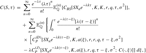
Equation (43) is indeed an integral equation since the unknown option price also appears under the time integral on the right-hand side, in particular through the ![]() term. This is in contrast to the pure diffusion case where the equation corresponding to (43) (when
term. This is in contrast to the pure diffusion case where the equation corresponding to (43) (when ![]() and so that the
and so that the ![]() term drops out) is simply an integral expression for the option price that can be evaluated once the free boundary has been determined.
term drops out) is simply an integral expression for the option price that can be evaluated once the free boundary has been determined.
The solution (43) is readily compared with that of Gukhal (2001), who derives (43) by generalizing the compound option approach of Kim (1990) to the jump-diffusion case. The three additive components of the call value in Eq. (43) each have a clear economic interpretation, as outlined by Gukhal (2001). The first term, ![]() , represents the European component of the American call option’s value, while the remaining two terms combine to form the total early exercise premium. The middle term is a natural extension of the early exercise premium that arises in the pure diffusion case. More specifically, this term calculates the dividend received when holding the underlying, less the interest payable on a loan of size
, represents the European component of the American call option’s value, while the remaining two terms combine to form the total early exercise premium. The middle term is a natural extension of the early exercise premium that arises in the pure diffusion case. More specifically, this term calculates the dividend received when holding the underlying, less the interest payable on a loan of size ![]() . Thus
. Thus ![]() captures the potential income to the option holder should the option be exercised to buy the underlying by borrowing
captures the potential income to the option holder should the option be exercised to buy the underlying by borrowing ![]() at the risk-free rate. The third term,
at the risk-free rate. The third term, ![]() , arises entirely due to the introduction of jumps in the price process for
, arises entirely due to the introduction of jumps in the price process for ![]() , and captures the rebalancing costs incurred by the option holder whenever the price of the underlying jumps down from the stopping region into the continuation region as illustrated in Figure 2.
, and captures the rebalancing costs incurred by the option holder whenever the price of the underlying jumps down from the stopping region into the continuation region as illustrated in Figure 2.
In Eq. (43), the value of the American call option is expressed as a function of the underlying asset price ![]() , and time to maturity
, and time to maturity ![]() . As we have already noted, Eq. (43) also depends upon the unknown early exercise boundary,
. As we have already noted, Eq. (43) also depends upon the unknown early exercise boundary, ![]() . By requiring the expression for
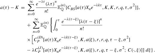
. By requiring the expression for ![]() to satisfy the early exercise boundary condition (20), we can derive the integral equation for
to satisfy the early exercise boundary condition (20), we can derive the integral equation for ![]() , namely
, namely
 (44)
(44)
Note that the integral Eq. (44) depends upon the unknown call value ![]() , which arises entirely from the integral terms that have been introduced by the presence of jumps in the dynamics for
, which arises entirely from the integral terms that have been introduced by the presence of jumps in the dynamics for ![]() .
.
The structure of the integral equation system consisting of (43) and (44) can be made more transparent by writing it succinctly as
![]() (45)
(45)
![]() (46)
(46)
where the definitions of the functions ![]() and
and ![]() can be inferred from the right-hand sides of Eqs. (43) and (44), respectively. The interdependence of (45) and (46) is obvious, and it is this interdependence that makes numerical implementation more involved than for the corresponding no-jump problem. There the dependence is sequential, that is, first one solves for the free boundary, which then feeds into an integral expression for the option price. In fact, Eqs. (43) and (44) form a linked system of non-linear Volterra integral equations of the second kind. Thus in order to implement these integral equations for the free boundary and call price, we need to develop numerical techniques to solve the linked integral equation system (43) and (44).
can be inferred from the right-hand sides of Eqs. (43) and (44), respectively. The interdependence of (45) and (46) is obvious, and it is this interdependence that makes numerical implementation more involved than for the corresponding no-jump problem. There the dependence is sequential, that is, first one solves for the free boundary, which then feeds into an integral expression for the option price. In fact, Eqs. (43) and (44) form a linked system of non-linear Volterra integral equations of the second kind. Thus in order to implement these integral equations for the free boundary and call price, we need to develop numerical techniques to solve the linked integral equation system (43) and (44).
Before concluding this subsection, we present an alternative form for the double integral involving the function ![]() in Eq. (40) and defined in (41).
in Eq. (40) and defined in (41).
From an economic point of view, the modified representation in (47) is less intuitive than the original; however, it offers significant advantages when attempting to evaluate (40) numerically for specific forms of ![]() . In particular, we will see in Section 3.5 that when
. In particular, we will see in Section 3.5 that when ![]() is the log-normal density function given by Merton (1976), the innermost integral in (47) can be evaluated analytically. In this way we are able to reduce (47) to a one-dimensional integral, which makes the task of numerically evaluating (47) much simpler. We remind the reader that the
is the log-normal density function given by Merton (1976), the innermost integral in (47) can be evaluated analytically. In this way we are able to reduce (47) to a one-dimensional integral, which makes the task of numerically evaluating (47) much simpler. We remind the reader that the ![]() term in turn must be integrated over time to maturity so that altogether the jump term would in this case involve the evaluation of a double integral.
term in turn must be integrated over time to maturity so that altogether the jump term would in this case involve the evaluation of a double integral.
3.4 Limit of the Early Exercise Boundary at Expiry
In order to implement numerical schemes we need to know the value of the free boundary just prior to expiry, at ![]() . Early literature, for instance, Amin (1993) and Carr and Hirsa (2003), simply assumed that this limit is identical to the corresponding pure diffusion case. However, Chiarella and Ziogas (2009) show that this limit is in fact more subtle. They derive the limit by analyzing the inhomogeneous term in the PIDE (23), and find that the presence of jumps does in fact have an impact on the early exercise boundary at expiry. This difference is expressed analytically in Proposition 3.7 below, and is based on the analysis of Wilmott et al. (1993). The simple, intuitive method used here is taken from Chiarella et al. (2004) who demonstrate that the approach of Wilmott et al. (1993) is equivalent to setting the inhomogeneous term in Jamshidian’s (1992) form for the PDE to zero, setting
. Early literature, for instance, Amin (1993) and Carr and Hirsa (2003), simply assumed that this limit is identical to the corresponding pure diffusion case. However, Chiarella and Ziogas (2009) show that this limit is in fact more subtle. They derive the limit by analyzing the inhomogeneous term in the PIDE (23), and find that the presence of jumps does in fact have an impact on the early exercise boundary at expiry. This difference is expressed analytically in Proposition 3.7 below, and is based on the analysis of Wilmott et al. (1993). The simple, intuitive method used here is taken from Chiarella et al. (2004) who demonstrate that the approach of Wilmott et al. (1993) is equivalent to setting the inhomogeneous term in Jamshidian’s (1992) form for the PDE to zero, setting ![]() , and solving for the free boundary.
, and solving for the free boundary.
It is worthwhile to observe that when ![]() Eq. (48) simplifies to the limit derived by Kim (1990) for the pure diffusion American call free boundary. Note that (48) is an implicit expression for
Eq. (48) simplifies to the limit derived by Kim (1990) for the pure diffusion American call free boundary. Note that (48) is an implicit expression for ![]() , but it can be solved quickly and accurately using standard root-finding techniques. Furthermore, as
, but it can be solved quickly and accurately using standard root-finding techniques. Furthermore, as ![]() the solution to the implicit part of Eq. (48) increases without bound. Thus when
the solution to the implicit part of Eq. (48) increases without bound. Thus when ![]() ,
, ![]() becomes infinite, and we observe the well-known property that it is never optimal to exercise an American call option early in the absence of dividends.
becomes infinite, and we observe the well-known property that it is never optimal to exercise an American call option early in the absence of dividends.
Before concluding this subsection, we shall take a closer look at the properties of Eq. (48), specifically with a view to better understanding the solution to
![]() (49)
(49)
where

Once (49) is solved, then the ![]() operator can be applied. Since the value of the underlying is always non-negative, we consider the domain
operator can be applied. Since the value of the underlying is always non-negative, we consider the domain ![]() when solving (49). It is not possible to provide a simple, explicit summary of the behavior of (49) for various values of
when solving (49). It is not possible to provide a simple, explicit summary of the behavior of (49) for various values of ![]() , because the integral terms depend upon
, because the integral terms depend upon ![]() , and the function
, and the function ![]() involves the parameters
involves the parameters ![]() and
and ![]() , as well as the jump-size density
, as well as the jump-size density ![]() .
.
First, we see that it is simple to evaluate ![]() at the limits of the domain. Specifically, we can show that
at the limits of the domain. Specifically, we can show that
![]() (50)
(50)
and
![]() (51)
(51)
Thus for ![]() to be finite at each extremity of the domain, it is sufficient that we have
to be finite at each extremity of the domain, it is sufficient that we have ![]() . In this case, it is clear that
. In this case, it is clear that ![]() is continuous, and (49) will have at least one solution. Since
is continuous, and (49) will have at least one solution. Since ![]() appears only in the limits of the integral terms over the density
appears only in the limits of the integral terms over the density ![]() within
within ![]() , we can safely claim that the behavior of
, we can safely claim that the behavior of ![]() with respect to
with respect to ![]() will be bounded by the behavior of
will be bounded by the behavior of ![]() . Further exploration appears difficult without specifying the form of
. Further exploration appears difficult without specifying the form of ![]() , and we provide a more detailed analysis in Section 3.5.
, and we provide a more detailed analysis in Section 3.5.
3.5 American Call with Log-Normal Jumps
Before we begin exploring a numerical solution method for the integral equation system (43) and (44), we shall consider the specific example when the jump-size density, ![]() is a log-normal distribution as in the original model of Merton (1976). The probability density function for
is a log-normal distribution as in the original model of Merton (1976). The probability density function for ![]() is given by
is given by
 (52)
(52)
where we set ![]() , and
, and ![]() is the variance of
is the variance of ![]() . Furthermore we note that for this choice of
. Furthermore we note that for this choice of ![]() we have
we have ![]() .
.
The last term of (53), which involves a double integral, may be further simplified before implementing (53) numerically.
We note that in the form (54) the ![]() term in (53) now only involves a single integral, which results in a considerable saving in computational effort.
term in (53) now only involves a single integral, which results in a considerable saving in computational effort.
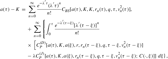
By use of (44), the integral equation for the early exercise boundary, ![]() , in the case of log-normal jump sizes, is given by
, in the case of log-normal jump sizes, is given by
 (56)
(56)
where ![]() and
and ![]() are given by (39) and (54), respectively.
are given by (39) and (54), respectively.
3.5.1 Delta for the American Call
We now provide one further result regarding the delta of the American call option, ![]() . This quantity is obviously important for hedging purposes, but it is also required by the numerical algorithm we consider in Section 3.7.
. This quantity is obviously important for hedging purposes, but it is also required by the numerical algorithm we consider in Section 3.7.
By differentiating (53) with respect to ![]() , we find that
, we find that
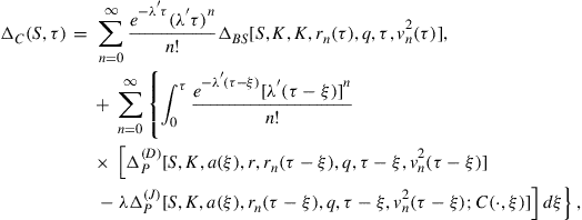 (57)
(57)
where
 (58)
(58)
 (59)
(59)
and we note that ![]() . Once we have found the price and free boundary for the American call option, we can readily evaluate (57) numerically to find delta.
. Once we have found the price and free boundary for the American call option, we can readily evaluate (57) numerically to find delta.
3.6 Properties of the Free Boundary at Expiry
Since we are now considering a specific form for ![]() , we consider again the topic of analyzing the behavior of the early exercise boundary,
, we consider again the topic of analyzing the behavior of the early exercise boundary, ![]() , as
, as ![]() . First we evaluate (48) for the log-normal density
. First we evaluate (48) for the log-normal density ![]() .
.
To develop an understanding of the case where ![]() , we explore numerically the equation
, we explore numerically the equation
![]() (61)
(61)
where

and we recall that ![]() . It is not possible to provide a simple, explicit summary of the behavior of (61) for various values of
. It is not possible to provide a simple, explicit summary of the behavior of (61) for various values of ![]() because the cumulative normal density functions depend upon
because the cumulative normal density functions depend upon ![]() , and the function
, and the function ![]() involves the parameters
involves the parameters ![]() ,
, ![]() ,
, ![]() ,
, ![]() , and
, and ![]() , all of which have a significant impact on the value of
, all of which have a significant impact on the value of ![]() . Nevertheless, we can use numerical examples to offer some additional insight into the nature of the solution of (61).
. Nevertheless, we can use numerical examples to offer some additional insight into the nature of the solution of (61).
For log-normal jump-sizes we can show that
![]() (62)
(62)
When ![]() it is clear that
it is clear that ![]() is continuous, and (61) will have at least one solution. We can demonstrate by example that
is continuous, and (61) will have at least one solution. We can demonstrate by example that ![]() is not monotonic, nor is it strictly bounded by the end values in (62). This makes it difficult to prove that for
is not monotonic, nor is it strictly bounded by the end values in (62). This makes it difficult to prove that for ![]() Eq. (61) has at most one solution. Since
Eq. (61) has at most one solution. Since ![]() appears only inside cumulative normal functions within
appears only inside cumulative normal functions within ![]() , the behavior of
, the behavior of ![]() with respect to
with respect to ![]() will be bounded by the behavior of
will be bounded by the behavior of ![]() . We recall that
. We recall that ![]() and that
and that ![]() is a smooth, continuous function of
is a smooth, continuous function of ![]() for
for ![]() . From this we postulate that the function
. From this we postulate that the function ![]() will not display any oscillatory features within the domain under consideration.
will not display any oscillatory features within the domain under consideration.
To provide numerical evidence in support of our claims regarding Eq. (61), we now present a plot of (62) which is typical of what we have obtained for a range of empirically relevant parameter values. Setting ![]() ,
, ![]() , and
, and ![]() , we plot in Figure 3 the functions
, we plot in Figure 3 the functions ![]() and
and ![]() for various values of
for various values of ![]() and
and ![]() . When
. When ![]() and
and ![]() , we can see that
, we can see that ![]() . On the other hand, when
. On the other hand, when ![]() and
and ![]() , we now have
, we now have ![]() . In both cases it is clear that
. In both cases it is clear that ![]() is not bounded by these endpoint values, and we can see that the relative values of
is not bounded by these endpoint values, and we can see that the relative values of ![]() and
and ![]() directly influence the values of
directly influence the values of ![]() and
and ![]() .
.
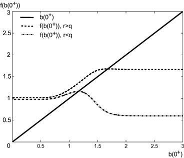
Figure 3 Behavior of Eq. (61) that determines the American call free boundary value at ![]() for various values of
for various values of ![]() with
with ![]() ,
, ![]() , and
, and ![]() . For
. For ![]() we set
we set ![]() , and for
, and for ![]() we take
we take ![]() .
.
Changing the values of the jump-parameters ![]() will vary the value of
will vary the value of ![]() . In addition, changes to
. In addition, changes to ![]() ,
, ![]() , and
, and ![]() will resize the curve
will resize the curve ![]() , although the basic shape remains unchanged. This claim is based on further numerical examples, which can be found in Chiarella and Ziogas (2009).
, although the basic shape remains unchanged. This claim is based on further numerical examples, which can be found in Chiarella and Ziogas (2009).
The last and most important scenario we consider here is when ![]() . In this case,
. In this case, ![]() is no longer finite, instead increasing without bound as
is no longer finite, instead increasing without bound as ![]() . Figure 4 demonstrates the behavior of
. Figure 4 demonstrates the behavior of ![]() with
with ![]() for a different selection of parameter values. It is clear from the plot that there is no solution to
for a different selection of parameter values. It is clear from the plot that there is no solution to ![]() . Furthermore, the only way that Eq. (61) will be satisfied when
. Furthermore, the only way that Eq. (61) will be satisfied when ![]() is by taking the limit as
is by taking the limit as ![]() , in which case both sides of (61) will increase without bound. This reflects in yet another way the fact that when
, in which case both sides of (61) will increase without bound. This reflects in yet another way the fact that when ![]() , the free boundary at
, the free boundary at ![]() becomes infinite, and it is never optimal to exercise an American call early in the absence of dividends.
becomes infinite, and it is never optimal to exercise an American call early in the absence of dividends.
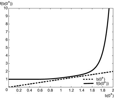
Figure 4 Behavior of Eq. (61) that determines the American call free boundary value at ![]() when
when ![]() . Other parameter values are
. Other parameter values are ![]() ,
, ![]() , and
, and ![]() .
.
3.7 Numerical Implementation
We now provide a numerical scheme with which to evaluate the linked integral equation system for the option price and free boundary formed by (53–56). The proposed method is an extension of the quadrature scheme used by Kallast and Kivinukk (2003) for the pure diffusion case. Here we focus on the adjustments that are needed to deal with the introduction of jumps into the dynamics for ![]() . We first discretize the time to maturity variable,
. We first discretize the time to maturity variable, ![]() , into
, into ![]() equally spaced intervals of length
equally spaced intervals of length ![]() . Thus
. Thus ![]() for
for ![]() , and
, and ![]() . We denote the call price profile at time step
. We denote the call price profile at time step ![]() by
by ![]() , and similarly the free boundary at time step
, and similarly the free boundary at time step ![]() by
by ![]() =
= ![]() . Using a standard numerical technique that is applied to Volterra integral equations, we can solve the system (53–56) for increasing values of
. Using a standard numerical technique that is applied to Volterra integral equations, we can solve the system (53–56) for increasing values of ![]() , until eventually the entire free boundary and price profile are found. When calculating the infinite summations, we continue adding terms until the size of the Poisson coefficient for a given value of
, until eventually the entire free boundary and price profile are found. When calculating the infinite summations, we continue adding terms until the size of the Poisson coefficient for a given value of ![]() is less than
is less than ![]() . For the parameter values considered here, this typically results in the use of around 30 terms in the summation. In order to start the algorithm we require the initial value of
. For the parameter values considered here, this typically results in the use of around 30 terms in the summation. In order to start the algorithm we require the initial value of ![]() , which is simply the payoff function, and
, which is simply the payoff function, and ![]() , where
, where ![]() , which is given by Eq. (60).
, which is given by Eq. (60).
Since the integral term in (54) depends upon ![]() , an approximation will be needed for
, an approximation will be needed for ![]() . At each time step we have found that a suitable approximation is given by
. At each time step we have found that a suitable approximation is given by ![]() , which is simply the American call price at the previous time step. The price at the
, which is simply the American call price at the previous time step. The price at the ![]() time step is calculated for a suitably large number of evenly spaced
time step is calculated for a suitably large number of evenly spaced ![]() values. Here we use 25 points in the range
values. Here we use 25 points in the range ![]() . All necessary interpolation is conducted using cubic splines fitted locally through seven values of
. All necessary interpolation is conducted using cubic splines fitted locally through seven values of ![]() . We then use Newton’s method to solve for the early exercise boundary, as in Kallast and Kivinukk (2003), with two necessary additions. The first addition addresses the evaluation of the inner integral (54) over the interval
. We then use Newton’s method to solve for the early exercise boundary, as in Kallast and Kivinukk (2003), with two necessary additions. The first addition addresses the evaluation of the inner integral (54) over the interval ![]() . This is computed using Gaussian integration of moments, with parameter
. This is computed using Gaussian integration of moments, with parameter ![]() . Full details of this Gauss quadrature scheme can be found in Abramowitz and Stegun (1970) (Chapter 25, p. 921). The second addition relates to finding the derivative of (56) with respect to
. Full details of this Gauss quadrature scheme can be found in Abramowitz and Stegun (1970) (Chapter 25, p. 921). The second addition relates to finding the derivative of (56) with respect to ![]() for use in Newton’s method. This is given by (57) for
for use in Newton’s method. This is given by (57) for ![]() , evaluated at
, evaluated at ![]() . Since it is difficult to determine the limit of the integrands in (57) as
. Since it is difficult to determine the limit of the integrands in (57) as ![]() , we resolve this by taking the limits as
, we resolve this by taking the limits as ![]() for the option price integrands in (53) and differentiating these with respect to
for the option price integrands in (53) and differentiating these with respect to ![]() , as is done by Kallast and Kivinukk (2003). These limits are all finite, including the new limit required for the jump-related integral term, and the required derivatives are easily determined. Since we need to evaluate the expression (57) for
, as is done by Kallast and Kivinukk (2003). These limits are all finite, including the new limit required for the jump-related integral term, and the required derivatives are easily determined. Since we need to evaluate the expression (57) for ![]() for use in Newton’s method, there is no significant additional computation time required to evaluate the American call delta once the free boundary has been estimated.
for use in Newton’s method, there is no significant additional computation time required to evaluate the American call delta once the free boundary has been estimated.
Having determined the discretized forms for the price and delta of ![]() , we then use Newton’s method to solve for
, we then use Newton’s method to solve for ![]() . Before proceeding to the next time step, we use
. Before proceeding to the next time step, we use ![]() to calculate a new approximation for
to calculate a new approximation for ![]() , which is required when evaluating the double integral term at all subsequent time steps. This update for
, which is required when evaluating the double integral term at all subsequent time steps. This update for ![]() is essential to ensure that the estimated free boundary remains monotonic. Note that as the value of
is essential to ensure that the estimated free boundary remains monotonic. Note that as the value of ![]() increases, the computational burden will also increase at a “faster than linear” rate (the reason being that the integration at step
increases, the computational burden will also increase at a “faster than linear” rate (the reason being that the integration at step ![]() depends on all values of
depends on all values of ![]() and
and ![]() for
for ![]() ).
).
It should be noted that the proposed numerical scheme does not involve any iterations with respect to the approximation of the integral term. It is possible to improve the accuracy of the algorithm by updating the approximation for the integral term at the ![]() th time step using the most recently computed estimates for
th time step using the most recently computed estimates for ![]() and
and ![]() . In practice we have found that such an iteration does not add significantly to the accuracy of the results (up to the order of accuracy considered in Section 3.8), and that computation time is at least doubled by the introduction of the iteration process. Thus we have chosen not to iterate with respect to the integral term approximation.
. In practice we have found that such an iteration does not add significantly to the accuracy of the results (up to the order of accuracy considered in Section 3.8), and that computation time is at least doubled by the introduction of the iteration process. Thus we have chosen not to iterate with respect to the integral term approximation.
To explore the efficiency of the proposed numerical integration method, we compare it with two alternative numerical methods. The first method involves a finite difference solution for the PIDE (17). We apply the Crank-Nicolson scheme to all terms except for the integral. We initially estimate the integral term by approximating ![]() with the explicit approximation
with the explicit approximation ![]() , as in Carr and Hirsa (2003). We then evaluate the integral using the Hermite-Gauss quadrature scheme (see Abramowitz and Stegun, 1970). The resulting tridiagonal matrix is inverted using LU-decomposition, and the early exercise condition is then applied to the solution at each time step. An evenly spaced grid is used, and the free boundary is estimated at each time step using cubic spline interpolation of the price profile, combined with the bisection method.
, as in Carr and Hirsa (2003). We then evaluate the integral using the Hermite-Gauss quadrature scheme (see Abramowitz and Stegun, 1970). The resulting tridiagonal matrix is inverted using LU-decomposition, and the early exercise condition is then applied to the solution at each time step. An evenly spaced grid is used, and the free boundary is estimated at each time step using cubic spline interpolation of the price profile, combined with the bisection method.
To improve the accuracy of the Crank-Nicolson solution, we use a two-step procedure at each time step, details of which are given by Chiarella and Ziogas (2009).
The second method we consider is the method of lines approach as presented by Meyer (1998). Meyer only considers discrete jump-size distributions. Here we extend this method to allow for a continuous jump-size density, ![]() , again evaluating the integral term using a Hermite-Gauss quadrature scheme, combined with local cubic spline interpolation of the price profile at each iteration. The method of lines readily provides estimates for both the price and delta for the American call option, without the need for additional computation. Unlike the Crank-Nicolson scheme, the method of lines solution is allowed to iterate until the largest observed change in the option price profile is less than
, again evaluating the integral term using a Hermite-Gauss quadrature scheme, combined with local cubic spline interpolation of the price profile at each iteration. The method of lines readily provides estimates for both the price and delta for the American call option, without the need for additional computation. Unlike the Crank-Nicolson scheme, the method of lines solution is allowed to iterate until the largest observed change in the option price profile is less than ![]() . The scheme we use is second-order accurate in time, and a first-order scheme is applied for the first three time steps.
. The scheme we use is second-order accurate in time, and a first-order scheme is applied for the first three time steps.
3.8 Numerical Results
To analyze the efficiency of the numerical integration method, we compute the price and delta of an American call option with 6 months to maturity, and a strike price of ![]() . The global variance11 of returns,
. The global variance11 of returns, ![]() , is set equal to
, is set equal to ![]() . The jump intensity is set to
. The jump intensity is set to ![]() , and the jump variance is
, and the jump variance is ![]() . We then consider six different parameter sets, specifically
. We then consider six different parameter sets, specifically ![]() taking values of 0.95, 1.00, and 1.04, along with the combinations
taking values of 0.95, 1.00, and 1.04, along with the combinations ![]() ,
, ![]() and
and ![]() ,
, ![]() . Note that
. Note that ![]() implies upward jumps on average, and
implies upward jumps on average, and ![]() implies downward jumps on average. When
implies downward jumps on average. When ![]() , the expected price change from a jump is zero. The diffusion coefficient,
, the expected price change from a jump is zero. The diffusion coefficient, ![]() , is chosen such that the global variance was preserved for varying values of
, is chosen such that the global variance was preserved for varying values of ![]() . Table 1 summarizes the values of
. Table 1 summarizes the values of ![]() used to ensure that the global variance was the same for each combination of
used to ensure that the global variance was the same for each combination of ![]() and
and ![]() .
.
Table 1
Parameter values used for the diffusion variance and jump component. The global variance is fixed at ![]() , determined by
, determined by ![]() .
.

We compute the root mean-square error (RMSE) using option prices and deltas with ![]() , and
, and ![]() . This is repeated for each of the six parameter sets, from which the average runtime and RMSE are then calculated. Note that in all cases the runtimes include the time required to compute the free boundary, price, and delta for the American call. For the integration method we use 20 integration points for the Gauss quadrature scheme, and consider a sequence of 10 different time step values, with
. This is repeated for each of the six parameter sets, from which the average runtime and RMSE are then calculated. Note that in all cases the runtimes include the time required to compute the free boundary, price, and delta for the American call. For the integration method we use 20 integration points for the Gauss quadrature scheme, and consider a sequence of 10 different time step values, with ![]() .
.
For the Crank-Nicolson method the integral term is approximated using 50 integration points, and we again use 10 time step values, with ![]() . We set the number of space steps equal to double the number of time steps. Similarly, we use 50 integration points to estimate the integral term in the method of lines. We also use 10 time step values, with
. We set the number of space steps equal to double the number of time steps. Similarly, we use 50 integration points to estimate the integral term in the method of lines. We also use 10 time step values, with ![]() , and the number of space steps is set to five times the number of time steps. The code for all methods has been implemented using LAHEYTMFORTRAN 95 running on a PC with a Pentium 4 2.40 GHz processer, 512 MB of RAM, and running the Windows XP Professional operating system.
, and the number of space steps is set to five times the number of time steps. The code for all methods has been implemented using LAHEYTMFORTRAN 95 running on a PC with a Pentium 4 2.40 GHz processer, 512 MB of RAM, and running the Windows XP Professional operating system.
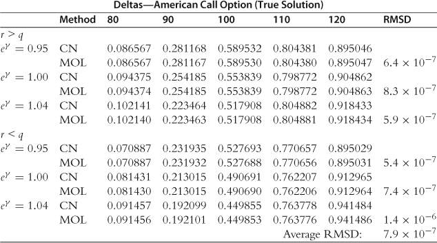
In assessing the efficiency of the numerical integration method, we use a Crank-Nicolson solution with 10,000 time steps and 5000 space steps for the true solution. Since the numerical integration scheme requires evaluation of the option delta as part of the solution, it is also worthwhile to consider the efficiency with which delta is calculated. The true delta is estimated from the Crank-Nicolson solution using the central difference approximation for ![]() . To demonstrate that this is a valid choice for the true solution, we also compute the prices and deltas using the method of lines approach with 1000 time steps and 5000 space steps. As mentioned previously, the method of lines computes the price, delta, and early exercise boundary simultaneously. The prices are provided in Table 2, with the deltas given in Table 3. We also provide the root mean-square differences (RMSD) between the two methods for each set of parameters, along with an average RMSD value. In both cases we find that for the values of
. To demonstrate that this is a valid choice for the true solution, we also compute the prices and deltas using the method of lines approach with 1000 time steps and 5000 space steps. As mentioned previously, the method of lines computes the price, delta, and early exercise boundary simultaneously. The prices are provided in Table 2, with the deltas given in Table 3. We also provide the root mean-square differences (RMSD) between the two methods for each set of parameters, along with an average RMSD value. In both cases we find that for the values of ![]() under consideration these methods are consistent to at least four decimal places, and thus we conclude that the Crank-Nicolson method using 10,000 time steps and 5000 steps in the space variable provides a satisfactory estimate for the true price and delta.
under consideration these methods are consistent to at least four decimal places, and thus we conclude that the Crank-Nicolson method using 10,000 time steps and 5000 steps in the space variable provides a satisfactory estimate for the true price and delta.
Table 2
Demonstrating the accuracy of the true American call prices using the Crank-Nicolson method with 10,000 time steps and 5000 space steps. The method of lines solution uses 1000 time steps and 5000 space steps. The values used for ![]() and
and ![]() were
were ![]() and
and ![]() , with
, with ![]() and
and ![]() . Other parameter values used are given in Table 1.
. Other parameter values used are given in Table 1.
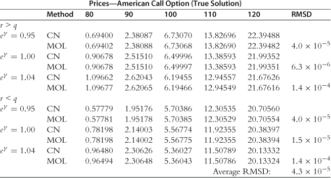
Table 3
Demonstrating the accuracy of the true American call deltas found by applying a central difference approximation to the price estimates given by the Crank-Nicolson method with 10,000 time steps and 5000 space steps. The method of lines solution uses 1000 time steps and 5000 space steps. The values used for ![]() and
and ![]() were
were ![]() and
and ![]() , with
, with ![]() and
and ![]() . Other parameter values used are given in Table 1.
. Other parameter values used are given in Table 1.
The relative efficiency of each method is shown in Figure 5 by comparing the RMSE as a function of runtime. Figure 5a shows the average RMSE error for the American call price, and Figure 5b displays the same information for the delta. Note that the average runtimes for each discretization level are the same in Figure 5a and b since the price and delta were found using a single algorithm. Firstly, we find that for the parameters and discretizations considered, the numerical integration method consistently displays greater efficiency than the Crank-Nicolson scheme for the American call price, and furthermore, numerical integration is more efficient than Crank-Nicolson when computing delta for computation times of up to 50 s.
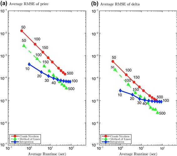
Figure 5 Comparing the efficiency of numerical integration, Crank-Nicolson and the method of lines for the price and delta of American call options with log-normal jump sizes. We set ![]() , and
, and ![]() . The RMSE is found using
. The RMSE is found using ![]() , and
, and ![]() . The average RMSE and runtimes have been determined using six parameter sets, with
. The average RMSE and runtimes have been determined using six parameter sets, with ![]() ,
, ![]() , and
, and ![]() ,
, ![]() , along with
, along with ![]() , and
, and ![]() . (a) displays the price efficiency, while (b) shows the delta efficiency. Numbers on the plot indicate the time steps associated with a given point.
. (a) displays the price efficiency, while (b) shows the delta efficiency. Numbers on the plot indicate the time steps associated with a given point.
We find that the method of lines consistently outperforms the Crank-Nicolson scheme, and in the majority of cases, the delta values computed by the method of lines are more accurate than those obtained using numerical integration. When computing prices for runtimes of between 1 and 20 s, however, numerical integration is able to outperform the method of lines. We also note that the numerical integration algorithm has a slower rate of convergence for the delta relative to the other two methods. This could be attributed to cumulative numerical integration error as the number of time steps, and hence integration points, is increased. The rate of convergence for the numerical integration method is clearly better when computing the option price.
Thus from Figure 512 we conclude that of the three methods under consideration, the method of lines is consistently more accurate for runtimes beyond 20 s. We also find that the numerical integration method consistently outperforms the Crank-Nicolson scheme when computing the option price, and is competitive with Crank-Nicolson when computing the delta for runtimes of less than 50 s. Thus we can see that a simple extension of the numerical integration scheme presented by Kallast and Kivinukk (2003) to include log-normal jumps produces a numerical method that is comparable with both the method of lines and the Crank-Nicolson scheme; however, there is room for improvement in the computation of delta, in particular when the number of time steps is increased beyond 40. We also note that since the magnitude of the RMSE is much larger for the option price, the best way to select the optimal numerical method is to maximize the pricing efficiency while being aware of the RMSE for the deltas. For example, for a runtime of 20 s the method of lines is more efficient than numerical integration, since both methods have similar pricing accuracy, but the method of lines offers a better delta estimate in this case. Alternatively, for a runtime of 5 s, numerical integration is the most efficient, since it provides better price estimates than the method of lines for the same accuracy in delta.
Chiarella and Ziogas (2009) give a lengthy discussion of the impact of jumps on the free boundary and option prices. However, lack of space prevents us from summarizing that discussion here so we refer the interested reader to the paper.
4 American Call Options under Jump-Diffusion and Stochastic Volatility Processes
In the previous section, we considered the simpler case of geometric Brownian motion plus jump-diffusion dynamics. In this section, we consider the case which combines stochastic volatility and jump-diffusion as was postulated in Section 2. In Section 4.1 we apply the method of lines which turns out to work quite well in the present context as the numerical results in Section 4.4 indicate. We refer the reader to Cheang et al. (2012) for the solution of this problem using integral transform methods. Of course this method can only work in a particular case whereas the method of lines can handle quite general situations.
4.1 Numerical Solution Using the Method of Lines
Given that it worked well in the jump-diffusion situation of Section 3.5 we continue with the method of lines, which has also been applied to the stochastic volatility case by Adolfsson et al. (2013). As we pointed out in Section 3.5 the method of lines also has the advantage that the price, free boundary, delta, and gamma are all found as part of the computation. The method of discretizing the PIDE is basically the same as in Section 3.5 and in this section we show how to adapt the implementations to also incorporate stochastic volatility. The section is a shortened version of Chiarella et al. (2009) to which we refer the reader for more details.
The key idea behind the method of lines is to replace an PIDE with an equivalent system of one-dimensional integro-differential equations (IDEs), whose solution is more readily obtained using numerical techniques. When volatility is constant, the system of IDEs is developed by discretizing the time derivative as discussed in Section 3.5. For the PIDE (11), we must also discretize the derivative terms involving the variance, ![]() , and adjust the algorithm for dealing with the integral term to cater for the fact that the option price and free surface also depend upon the variance
, and adjust the algorithm for dealing with the integral term to cater for the fact that the option price and free surface also depend upon the variance ![]() .
.
We begin by setting ![]() , where
, where ![]() . Typically we will set the maximum variance to be
. Typically we will set the maximum variance to be ![]() . Furthermore, as in Section 3.5 we discretize the time to expiry according to
. Furthermore, as in Section 3.5 we discretize the time to expiry according to ![]() , where
, where ![]() . We denote the option price along the variance line
. We denote the option price along the variance line ![]() and time line
and time line ![]() by
by ![]() , and set
, and set
![]() (63)
(63)
which is of course the option delta at the grid point.
We now select finite difference approximations for the derivative terms with respect to ![]() . For the second-order term, at the grid point
. For the second-order term, at the grid point ![]() we use the standard central difference scheme
we use the standard central difference scheme
![]() (64)
(64)
and for the cross-derivative term at the grid point ![]() we use the central difference approximation
we use the central difference approximation
![]() (65)
(65)
Since the coefficients of the second-order derivative terms go to zero as ![]() , we use an upwinding finite difference scheme (see Duffy, 2006, Chapter 8) for the first-order derivative term, such that, at the grid point
, we use an upwinding finite difference scheme (see Duffy, 2006, Chapter 8) for the first-order derivative term, such that, at the grid point ![]() we have
we have
 (66)
(66)
Since the second-order derivative terms both vanish as ![]() , upwinding helps to stabilize the finite difference scheme with respect to
, upwinding helps to stabilize the finite difference scheme with respect to ![]() .
.
The integral term in (11) at each grid point is estimated using numerical integration as in Section 3.5. Assuming, as in that section, that the jump sizes are log-normally distributed, with distribution ![]() 13 given by (52). Note that the method developed here could allow a wide range of choices for
13 given by (52). Note that the method developed here could allow a wide range of choices for ![]() , for instance, the double exponential distribution of Kou (2002).
, for instance, the double exponential distribution of Kou (2002).
Making the change of variable ![]() , the integral term in (11) becomes
, the integral term in (11) becomes
![]() (67)
(67)
We approximate (67) at the grid point ![]() with the discretization obtained by applying the Hermite-Gauss quadrature scheme, namely
with the discretization obtained by applying the Hermite-Gauss quadrature scheme, namely
 (68)
(68)
where ![]() and
and ![]() are the weights and abscissas for the Hermite-Gauss quadrature scheme with
are the weights and abscissas for the Hermite-Gauss quadrature scheme with ![]() integration points. As in Section 3.5 we refer the reader to Abramowitz and Stegun (1970) for the computation of the weights and abscissas. We interpolate for the required non-grid-point values of
integration points. As in Section 3.5 we refer the reader to Abramowitz and Stegun (1970) for the computation of the weights and abscissas. We interpolate for the required non-grid-point values of ![]() using cubic splines fitted in
using cubic splines fitted in ![]() along the line at the grid point (
along the line at the grid point (![]() ). We handle the discretization for the time derivative as in Section 3.5.
). We handle the discretization for the time derivative as in Section 3.5.
Applying (64–68) and the time discretization to the PIDE (11), we must now solve a system of second-order IDEs at each time step and variance grid point. For the first three steps, the IDE at the grid point ![]() and
and ![]() is
is
 (69)
(69)
and for all subsequent time steps the IDE is
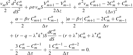 (70)
(70)
We require two boundary conditions in the ![]() -direction, one at
-direction, one at ![]() and the other at
and the other at ![]() . For large values of
. For large values of ![]() , the rate of change of the option price with respect to
, the rate of change of the option price with respect to ![]() diminishes. So for sufficiently large values of
diminishes. So for sufficiently large values of ![]() , one can treat this rate of change as zero without any impact on the accuracy of the solution at other values of
, one can treat this rate of change as zero without any impact on the accuracy of the solution at other values of ![]() . Thus we set
. Thus we set ![]() along the variance boundary
along the variance boundary ![]() . When
. When ![]() is zero, we fit a quadratic polynomial through the option prices at
is zero, we fit a quadratic polynomial through the option prices at ![]() ,
, ![]() , and
, and ![]() , and then use this to extrapolate an approximation of the price at
, and then use this to extrapolate an approximation of the price at ![]() . This provides us with a satisfactory estimate of the price along
. This provides us with a satisfactory estimate of the price along ![]() for the purpose of generating a stable solution for small values of
for the purpose of generating a stable solution for small values of ![]() .
.
After taking the boundary conditions into consideration, at each time step ![]() we must solve a system of
we must solve a system of ![]() second-order IDEs along the variance lines. This is done using a two-stage iterative scheme. As in Section 3.5 first we treat the IDEs as ODEs by using
second-order IDEs along the variance lines. This is done using a two-stage iterative scheme. As in Section 3.5 first we treat the IDEs as ODEs by using ![]() as an initial approximation for
as an initial approximation for ![]() in the integral term
in the integral term ![]() . We then solve the ODEs for increasing values of
. We then solve the ODEs for increasing values of ![]() , using the latest available estimates for
, using the latest available estimates for ![]() , and
, and ![]() . The initial estimates for
. The initial estimates for ![]() and
and ![]() are simply
are simply ![]() and
and ![]() . Otherwise we use the latest estimates for
. Otherwise we use the latest estimates for ![]() and
and ![]() found during the current iteration through the variance lines. We iterate until the price profile converges to a desired level of accuracy. Second, once the price has converged, we update the estimate of the integral term
found during the current iteration through the variance lines. We iterate until the price profile converges to a desired level of accuracy. Second, once the price has converged, we update the estimate of the integral term ![]() using the current price profile estimate, and repeat the process until convergence is obtained for both levels of iteration. We then proceed to the next time step.
using the current price profile estimate, and repeat the process until convergence is obtained for both levels of iteration. We then proceed to the next time step.
The generic first-order form for (69) and (70) is
![]() (71)
(71)
![]() (72)
(72)
where ![]() is a function of
is a function of ![]() ,
, ![]() ,
, ![]() ,
, ![]() ,
, ![]() ,
, ![]() , and
, and ![]() . We solve (71) and (72) using the Riccati transform (see Meyer and van der Hoek, 1997 for details).14 Note that we are only able to apply the Riccati transform to the system (71) and (72) provided that both equations are treated as ODEs. This is made possible by approximating
. We solve (71) and (72) using the Riccati transform (see Meyer and van der Hoek, 1997 for details).14 Note that we are only able to apply the Riccati transform to the system (71) and (72) provided that both equations are treated as ODEs. This is made possible by approximating ![]() using the values
using the values ![]() of the previous time step, as stated earlier, and then using an iterative technique in which the integral term is updated until the price converges. For later use we note that the right-hand sides of Eqs. (71) and (72), respectively, yield the delta and gamma at each point of the grid.
of the previous time step, as stated earlier, and then using an iterative technique in which the integral term is updated until the price converges. For later use we note that the right-hand sides of Eqs. (71) and (72), respectively, yield the delta and gamma at each point of the grid.
The Riccati transformation is given by
![]() (73)
(73)
where ![]() and
and ![]() are solutions to the initial value problems
are solutions to the initial value problems
![]() (74)
(74)
![]() (75)
(75)
and ![]() is the solution to
is the solution to
![]() (76)
(76)
where we denote the free boundary at grid point ![]() by
by ![]() .15 Since
.15 Since ![]() is independent of
is independent of ![]() , we begin by solving (74) and storing the solution. Next we solve (75) for increasing values of
, we begin by solving (74) and storing the solution. Next we solve (75) for increasing values of ![]() , ranging from
, ranging from ![]() , where we select
, where we select ![]() sufficiently large such that
sufficiently large such that ![]() will be guaranteed. We then step forward in
will be guaranteed. We then step forward in ![]() using the generated values of
using the generated values of ![]() and
and ![]() until we encounter the value
until we encounter the value ![]() such that16
such that16
![]() (77)
(77)
and thus ![]() is the value of the free boundary at grid point
is the value of the free boundary at grid point ![]() .17 Once
.17 Once ![]() has been determined we then solve (76) starting at
has been determined we then solve (76) starting at ![]() and sweeping back to
and sweeping back to ![]() . Finally we use the calculated values of
. Finally we use the calculated values of ![]() , and
, and ![]() in (73) to determine the option price at each grid point along the variance lines at time to maturity
in (73) to determine the option price at each grid point along the variance lines at time to maturity ![]() .
.
In Figure 6 we illustrate one sweep through the grid points on the ![]() plane. In Figure 7 we show the stencil for the typical grid point in Figure 6; this essentially shows the grid point values of
plane. In Figure 7 we show the stencil for the typical grid point in Figure 6; this essentially shows the grid point values of ![]() that enter the
that enter the ![]() term on the right-hand side of (72). Figure 8 then illustrates the solution of (75) along a line in the
term on the right-hand side of (72). Figure 8 then illustrates the solution of (75) along a line in the ![]() -direction from a typical grid point in the
-direction from a typical grid point in the ![]() plane.
plane.
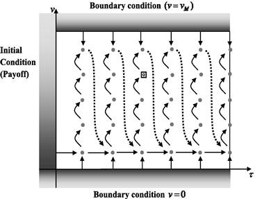
Figure 6 Illustrating one sweep of the solution scheme on a simple ![]() grid. The integral term of the jump size distribution is approximated as discussed in the text. The stencil for the typical point
grid. The integral term of the jump size distribution is approximated as discussed in the text. The stencil for the typical point ![]() is displayed in Figure 7.
is displayed in Figure 7.
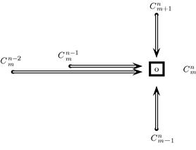
Figure 7 The stencil at a typical grid point ![]() of Figure 6. The stencil for
of Figure 6. The stencil for ![]() depends on the grid values
depends on the grid values ![]() .
.
4.2 Numerical Solution Using the Componentwise Splitting Method
Ikonen and Toivanen (2007) have proposed a non-standard finite difference method that involves discretization of the spot price on non-uniform grids in order to solve the American option pricing problem under stochastic volatility. We employ the same method, with the only difference being that we extend it to handle the integral over jumps term. Here, we give the basic details of the componentwise splitting method in order to make clear how the jump term is incorporated. We refer the reader to Ikonen and Toivanen (2007) (henceforth IT) for full details.
For a reference grid point ![]() , we have neighboring grid points at
, we have neighboring grid points at ![]() and at
and at ![]() , where
, where ![]() and
and ![]() are the local left and right grid step sizes for the spot price, respectively. We discuss later how these step sizes are chosen. In the variance direction we employ a uniform grid with the step size
are the local left and right grid step sizes for the spot price, respectively. We discuss later how these step sizes are chosen. In the variance direction we employ a uniform grid with the step size ![]() and, hence, neighboring grid points are at
and, hence, neighboring grid points are at ![]() and at
and at ![]() .
.
By use of the Taylor expansions at ![]() and
and ![]() , the first-order and second-order derivatives in the
, the first-order and second-order derivatives in the ![]() -direction are given by the finite difference approximations
-direction are given by the finite difference approximations
![]() (78)
(78)
and
![]() (79)
(79)
The first-order and second-order derivatives in the ![]() -direction are handled in the usual way with a central difference for the first-order derivative.
-direction are handled in the usual way with a central difference for the first-order derivative.
IT discuss the second-order cross-derivative terms when the correlation is positive; however, we wish to handle both the positive and negative correlation cases. Hence, here we detail the negative correlation case and refer the reader to IT for the case of positive correlation. By considering Taylor expansions at ![]() and
and ![]() IT obtain for the second-order cross-derivative terms the approximations
IT obtain for the second-order cross-derivative terms the approximations
 (80)
(80)
and
 (81)
(81)
which involve derivatives only in the ![]() - and
- and ![]() -directions. In order to obtain a discretization with the desired so-called M-Matrix properties (that is, positive diagonal elements and negative sub-diagonal and super-diagonal elements) IT suggest the convex combination
-directions. In order to obtain a discretization with the desired so-called M-Matrix properties (that is, positive diagonal elements and negative sub-diagonal and super-diagonal elements) IT suggest the convex combination
 (82)
(82)
of (80) and (81) for the second-order cross-derivative. The weighting parameter ![]() has a value between zero and one. For most of the grid points we use the weight
has a value between zero and one. For most of the grid points we use the weight ![]() . On the boundaries18
. On the boundaries18 ![]() where the boundary condition (7) is posed we use
where the boundary condition (7) is posed we use ![]() to avoid crossing the boundary in the
to avoid crossing the boundary in the ![]() -direction. On the boundaries
-direction. On the boundaries ![]() , where the boundary condition (9) is imposed, we use the weight
, where the boundary condition (9) is imposed, we use the weight ![]() to avoid crossing the boundary in the
to avoid crossing the boundary in the ![]() -direction. For small
-direction. For small ![]() the weight is set to zero to obtain the
the weight is set to zero to obtain the ![]() -Matrix property. We refer the reader to IT for a discussion analogous to the above for the positive correlation case.
-Matrix property. We refer the reader to IT for a discussion analogous to the above for the positive correlation case.
Using the approximation (82) for the cross-derivative in the partial differential equation (11), we obtain a form which contains only the partial derivatives in the ![]() -direction and in the
-direction and in the ![]() -direction. This intermediate form reads
-direction. This intermediate form reads
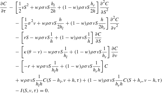 (83)
(83)
where the last item, ![]() , is the jump term from (67) which is approximated as in (68).
, is the jump term from (67) which is approximated as in (68).
A seven point finite difference stencil around the typical ![]() point, which is displayed in Figure 9, is obtained by using the finite difference approximations introduced in the previous part of this section for the spatial derivatives appearing in (83). We will discretize and solve (83) without jumps first and then we will add the jump term back later. The spatial discretization leads to a semi-discrete equation which has the matrix representation
point, which is displayed in Figure 9, is obtained by using the finite difference approximations introduced in the previous part of this section for the spatial derivatives appearing in (83). We will discretize and solve (83) without jumps first and then we will add the jump term back later. The spatial discretization leads to a semi-discrete equation which has the matrix representation
![]() (84)
(84)
where ![]() is a block tridiagonal
is a block tridiagonal ![]() matrix and
matrix and ![]() is a vector of length
is a vector of length ![]() .
.
Next, we implement the Crank-Nicolson method to discretize the semi-discrete problem (84) as
![]() (85)
(85)
where ![]() is the number of time steps and
is the number of time steps and ![]() is the identity matrix.
is the identity matrix.
After the discretization of the underlying PIDE with two spatial variables an approximate price of an American option can be obtained by solving the sequence of linear complementarity problems (LCPs) (see Wilmott et al., 1993)
 (86)
(86)
for ![]() . The matrices
. The matrices ![]() and
and ![]() in (86) are defined by (85) for the Crank-Nicolson method. The initial value
in (86) are defined by (85) for the Crank-Nicolson method. The initial value ![]() is given by the discrete form
is given by the discrete form ![]() of the payoff function
of the payoff function ![]() of the option, so that the
of the option, so that the ![]() th element of
th element of ![]() is given by
is given by
![]() (87)
(87)
In order to solve the sequence (86) of LCPs more efficiently, we implement the componentwise splitting method for LCPs based on the decomposition of the matrix ![]() in (84) according to
in (84) according to
![]() (88)
(88)
The matrices ![]() contain the couplings of the finite difference stencil in the
contain the couplings of the finite difference stencil in the ![]() -direction, in the
-direction, in the ![]() -direction, and in the
-direction, and in the ![]() -direction, respectively. We refer the reader to IT for the full details of this decomposition.
-direction, respectively. We refer the reader to IT for the full details of this decomposition.
We follow IT in using a second-order accurate splitting method by performing a Strang symmetrization (see Strang, 1968) for the splitting method which uses the Crank-Nicolson method. We choose to perform first a half time step with ![]() and then with
and then with ![]() , a full time step with
, a full time step with ![]() , and finally a half time step with
, and finally a half time step with ![]() and then with
and then with ![]() . The notations used are
. The notations used are
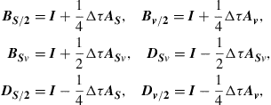 (89)
(89)
in terms of which the original LCP (86) is approximated by following five LCPs in successive directions:
![]() (90)
(90)
![]() (91)
(91)
where ![]() and
and ![]() run successively over the values
run successively over the values
![]()
and
![]()
while ![]() runs over the values
runs over the values ![]() .
.
We will omit the details of the implementations19 of the above system but again refer the reader to IT.
To be consistent with the Strang symmetrization given by (90) and (91), the evaluation of the integral term should also be decomposed and distributed among the five partial time steps. In fact, we add the integral term ![]() to the explicit terms20 of (90) separately and it is evaluated in a similar way as it is in Section 4.1 by using a cubic spline interpolation on the stock prices from the previous time step. The integral jump term is handled in the following way: first, we evaluate
to the explicit terms20 of (90) separately and it is evaluated in a similar way as it is in Section 4.1 by using a cubic spline interpolation on the stock prices from the previous time step. The integral jump term is handled in the following way: first, we evaluate ![]() at payoff from the previous time step or the result from the latest iteration; then we add 1/6 of
at payoff from the previous time step or the result from the latest iteration; then we add 1/6 of ![]() to the
to the ![]() -direction which is the explicit term of LCPs (90) for
-direction which is the explicit term of LCPs (90) for ![]() and
and ![]() ; we add another 1/6 of
; we add another 1/6 of ![]() to the
to the ![]() -direction which is the explicit term of LCPs (90) for
-direction which is the explicit term of LCPs (90) for ![]() and
and ![]() ; next we add 1/3 of
; next we add 1/3 of ![]() to the
to the ![]() -direction which is the explicit term of LCPs (90) for
-direction which is the explicit term of LCPs (90) for ![]() and
and ![]() ; and we add 1/6 of
; and we add 1/6 of ![]() to the
to the ![]() -direction which is the explicit term of LCPs (90) for
-direction which is the explicit term of LCPs (90) for ![]() and
and ![]() ; finally we add 1/6 of
; finally we add 1/6 of ![]() to the
to the ![]() -direction which is the explicit term of LCPs (90) for
-direction which is the explicit term of LCPs (90) for ![]() and
and ![]() . Now we have added a full time step integral to the original LCP (86). Next, we evaluate the integral term with cubic spline interpolation based on the new price and calculate the average difference of the successive iterations in the grid. We continue to add the integral terms to LCPs and to calculate the new price based on the new integral if the difference is larger than some tolerance; otherwise, we will proceed to the next time step.
. Now we have added a full time step integral to the original LCP (86). Next, we evaluate the integral term with cubic spline interpolation based on the new price and calculate the average difference of the successive iterations in the grid. We continue to add the integral terms to LCPs and to calculate the new price based on the new integral if the difference is larger than some tolerance; otherwise, we will proceed to the next time step.
4.3 Numerical Solution Using Finite Difference Method with PSOR
We have implemented a finite difference PSOR to find the benchmark prices of the American options. The implementation of PSOR is detailed in this subsection.
Three variables ![]() , and
, and ![]() are discretized as
are discretized as
![]()
The option prices at those discrete points thus are
![]()
with an initial condition:
![]()
Similar to the discussions in Ekstrom et al. (2009), we use central differences to approximate most of the first and second derivatives in the PDE but use the forward and backward finite difference approximations on the boundaries other than the time derivative in (11). Thus we set,

and

At ![]() , we fit a quadratic polynomial through the option prices at
, we fit a quadratic polynomial through the option prices at ![]() ,
, ![]() , and
, and ![]() which are the points closest to
which are the points closest to ![]() , and then use this to extrapolate an approximation of the price at
, and then use this to extrapolate an approximation of the price at ![]() . We use the boundary conditions
. We use the boundary conditions ![]() at the boundaries
at the boundaries ![]() . Those conditions are similarly handled to those in Section 4.1.
. Those conditions are similarly handled to those in Section 4.1.
All other derivative terms in the ![]() -direction vanish at
-direction vanish at ![]() due to the factor
due to the factor ![]() occurring in (11), and hence, these terms do not require further treatment.
occurring in (11), and hence, these terms do not require further treatment.
Boundary conditions at the boundaries ![]() and
and ![]() for a call option are
for a call option are
![]()
while those for a put option should be set as:
![]()
We follow Ikonen and Toivanen (2007) to indicate which grid point values we use to approximate the second-order mixed derivative in order to obtain non-positive off-diagonal weights in the finite difference stencil, which makes the matrix an M-matrix as far as possible.
In the above scheme a nine points ![]() stencil will be used. In order to simplify the algorithm and take into account the correlation
stencil will be used. In order to simplify the algorithm and take into account the correlation ![]() between the underlying asset and the variance, we use a seven points stencil instead and the mixed derivatives are approximated as
between the underlying asset and the variance, we use a seven points stencil instead and the mixed derivatives are approximated as ![]() by
by
 (92)
(92)
and when ![]() we have
we have
 (93)
(93)
The spatial discretization above leads to a semi-discrete equation which has the matrix representation
![]() (94)
(94)
where ![]() is a block tridiagonal
is a block tridiagonal ![]() matrix and
matrix and ![]() is a vector of length
is a vector of length ![]() .
.
Next, we implement a more general ![]() -scheme which includes the implicit (
-scheme which includes the implicit (![]() ), the Crank-Nicolson (
), the Crank-Nicolson (![]() ), and the explicit (
), and the explicit (![]() ) approaches to discretize the semi-discrete problem (94) as
) approaches to discretize the semi-discrete problem (94) as
![]() (95)
(95)
where ![]() is the number of time steps and
is the number of time steps and ![]() is the identity matrix.
is the identity matrix.
After the discretization of the underlying PIDE with two spatial variables an approximate price of an American option can be obtained by solving a sequence of linear complementarity problems (LCPs)
 (96)
(96)
for ![]() . The matrices
. The matrices ![]() and
and ![]() in (96) are defined by the left-hand side and right-hand side of (95), respectively. The initial value
in (96) are defined by the left-hand side and right-hand side of (95), respectively. The initial value ![]() is given by the discrete form
is given by the discrete form ![]() of the payoff function
of the payoff function ![]() of the option, so that the
of the option, so that the ![]() th element of
th element of ![]() is given by
is given by
![]() (97)
(97)
In order to avoid the oscillations that often occur with the CN scheme, we use the implicit Euler scheme (![]() ) for the first three time steps and then switch to the CN scheme (
) for the first three time steps and then switch to the CN scheme (![]() ) for the rest of the time steps. We have implemented a PSOR finite difference scheme (see Section 6.2.3 in Kwok (2008)) to solve the sequence (96) of LCPs. The jumps have been handled in the same way as in Section 4.2.
) for the rest of the time steps. We have implemented a PSOR finite difference scheme (see Section 6.2.3 in Kwok (2008)) to solve the sequence (96) of LCPs. The jumps have been handled in the same way as in Section 4.2.
In order to accelerate the convergence of the PSOR, we select the over-relaxation parameter ![]() in the algorithm. The free (or early exercise) boundary of the American option is obtained using Newton’s method. However, the option prices are updated with the American condition inside the PSOR, which makes it hard to obtain the free boundary. To solve this problem, original unprojected prices where the American condition is posed are saved and these prices are then used to obtain the free boundary later.
in the algorithm. The free (or early exercise) boundary of the American option is obtained using Newton’s method. However, the option prices are updated with the American condition inside the PSOR, which makes it hard to obtain the free boundary. To solve this problem, original unprojected prices where the American condition is posed are saved and these prices are then used to obtain the free boundary later.
4.4 Numerical Results
To demonstrate the performance of the method of lines algorithm outlined in Section 4.1 we implement the method for a given set of parameter values, chosen in order to best illustrate the impact that stochastic volatility and jump-diffusion may have on the early exercise boundary for an American call option. The parameter values used are listed in Table 4.
Table 4
Parameter values used for the American call option. The stochastic volatility (SV) parameters correspond to the Heston model. The jump-diffusion (JD) parameters correspond to the Merton model with log-normal jump sizes.

We consider the case where ![]() , and a time to maturity of 6 months, as this best demonstrates the changes that arise in the free boundary when jumps are introduced. The value of
, and a time to maturity of 6 months, as this best demonstrates the changes that arise in the free boundary when jumps are introduced. The value of ![]() is chosen intentionally large in order to emphasize the impact of stochastic volatility on the free boundary. We assume that jump sizes are log-normally distributed about a mean value of
is chosen intentionally large in order to emphasize the impact of stochastic volatility on the free boundary. We assume that jump sizes are log-normally distributed about a mean value of ![]() so that in a sense the jumps up and down average out. This allows us to focus on the impact that the Wiener correlation,
so that in a sense the jumps up and down average out. This allows us to focus on the impact that the Wiener correlation, ![]() , has on the free boundary. In addition, the small value of
, has on the free boundary. In addition, the small value of ![]() has been chosen so as to avoid further increases to the overall variance of
has been chosen so as to avoid further increases to the overall variance of ![]() .
.
When implementing the method of lines we take the following case as an example to show its convergence pattern. We use ![]() time steps and
time steps and ![]() variance lines, up to a maximum variance of
variance lines, up to a maximum variance of ![]() . We take a non-uniform grid in
. We take a non-uniform grid in ![]() , splitting the domain into three intervals. Given that the strike price is
, splitting the domain into three intervals. Given that the strike price is ![]() , the maximum value for
, the maximum value for ![]() is set to 400, with a total of 1138 grid points (denoted by
is set to 400, with a total of 1138 grid points (denoted by ![]() ), distributed between the three intervals such that there are 40 points for
), distributed between the three intervals such that there are 40 points for ![]() , there are 198 points for
, there are 198 points for ![]() , and finally 900 grid points for
, and finally 900 grid points for ![]() .
.
For the Hermite-Gauss quadrature scheme in (68) we use ![]() abscissa points. All iterative calculations utilize the stopping condition that the maximum over all
abscissa points. All iterative calculations utilize the stopping condition that the maximum over all ![]() of
of ![]() is less than
is less than ![]() , where the superscript
, where the superscript ![]() denotes the solution at the
denotes the solution at the ![]() th iteration. We note that for the parameter values given in Table 4, the solution along the variance lines typically converges in less than
th iteration. We note that for the parameter values given in Table 4, the solution along the variance lines typically converges in less than ![]() iterations, and convergence with respect to updating the integral term (67) generally needs no more than six iterations. Furthermore, the number of iterations along the variance lines reduces by more than a quarter after the first update of the integral term and continues to reduce by more than a half after each update of the integral term. A typical sequence is shown in Table 5. It is also of interest to observe how the total number of variance iterations changes as the number of variance lines changes; this effect is shown in Table 6. It seems that the number of variance iterations increases faster than the number of lines in the
iterations, and convergence with respect to updating the integral term (67) generally needs no more than six iterations. Furthermore, the number of iterations along the variance lines reduces by more than a quarter after the first update of the integral term and continues to reduce by more than a half after each update of the integral term. A typical sequence is shown in Table 5. It is also of interest to observe how the total number of variance iterations changes as the number of variance lines changes; this effect is shown in Table 6. It seems that the number of variance iterations increases faster than the number of lines in the ![]() -direction. This deterioration in convergence is similar to that observed in a standard Gauss-Seidel scheme, and is probably due to the fact that as in Gauss-Seidel iteration we are using the latest updates for the values as we step through the (
-direction. This deterioration in convergence is similar to that observed in a standard Gauss-Seidel scheme, and is probably due to the fact that as in Gauss-Seidel iteration we are using the latest updates for the values as we step through the (![]() ) grid. It is also worth noting that of all the components within the iterative scheme, computing the integral term (68) is the most computationally intensive, since we must perform
) grid. It is also worth noting that of all the components within the iterative scheme, computing the integral term (68) is the most computationally intensive, since we must perform ![]() extrapolations of
extrapolations of ![]() with respect to
with respect to ![]() at every point in the
at every point in the ![]() grid. Thus we are required to fit a total of
grid. Thus we are required to fit a total of ![]() cubic splines at each iteration with respect to the integral term, and each spline is fitted using every grid point in
cubic splines at each iteration with respect to the integral term, and each spline is fitted using every grid point in ![]() .
.
Table 5
A typical convergence pattern for the method of lines iterative procedure. The parameter values are given in Table 4.
| Integral Iteration | Variance Iterations |
| 1st | 82 |
| 2nd | 61 |
| 3rd | 39 |
| 4th | 18 |
| 5th | 3 |
| 6th | 1 |
| Total SV iterations | 204 |
Table 6
The changes of the number of required variance iterations with respect to the changes in the ![]() -direction.
-direction.

We refer the reader to Chiarella et al. (2009) for a graph of the free surface, where we note that the free surface generated by the method of lines is smooth, even when jumps are present, a feature not often displayed in the free boundary estimates generated using finite difference methods, such as Ikonen and Toivanen (2004).
We contrast the relative pricing accuracy of both the method of lines (MOL) and componentwise splitting (CS) methods. Using the parameter values in Table 4, and setting the spot variance to ![]() , we generate American call option prices for values of
, we generate American call option prices for values of ![]() equal to
equal to ![]() , and
, and ![]() using the three numerical methods discussed above: the method of lines as outlined in Section 4.1, a componentwise splitting (CS) approach which is detailed in Section 4.2 and the Crank-Nicolson scheme where the system of difference equations is solved using PSOR in Section 4.3. The integral term is approximated in the same manner as for the MOL and CS; we iterate at each time step and update the integral term until the price profile converges.21 We use
using the three numerical methods discussed above: the method of lines as outlined in Section 4.1, a componentwise splitting (CS) approach which is detailed in Section 4.2 and the Crank-Nicolson scheme where the system of difference equations is solved using PSOR in Section 4.3. The integral term is approximated in the same manner as for the MOL and CS; we iterate at each time step and update the integral term until the price profile converges.21 We use ![]() abscissa points for the integral term in all methods. We experimented with each of the above methods with an increase in the number of abscissa points from
abscissa points for the integral term in all methods. We experimented with each of the above methods with an increase in the number of abscissa points from ![]() to
to ![]() , but this led to a significant increase in the run time with no significant change in the option prices.
, but this led to a significant increase in the run time with no significant change in the option prices.
For both finite difference methods, we find that it is more efficient to update the integral term external to solving the system of difference equations.22 Note that while we do not prove convergence for these iterative schemes with respect to the value of the integral term, convergence is always observed in practice for the parameter values under consideration. The source code for all methods was implemented using NAG Fortran with the IMSL library running on the UTS, Faculty of Business F&E HPC Linux Cluster which consists of eight nodes running Red Hat Enterprise Linux 4.0 (64 bit) with ![]() GHz 4 MB Cache Xeon 5160 (dual core) Processors, 8 GB 667 MHz DDR2-RAM.
GHz 4 MB Cache Xeon 5160 (dual core) Processors, 8 GB 667 MHz DDR2-RAM.
In the following, we treat the solution for the price from PSOR with 1000 time steps, 3000 variance steps, and 6000 share price steps as the “true” solution for the purpose of comparing the efficiency of both the MOL and CS methods. We treat the delta and gamma from the MOL with 500 time steps, 1000 variance steps, and ![]() share price steps as the “true” deltas and gammas. We compute the root mean-square relative difference23 (RMSRD) using the option prices with
share price steps as the “true” deltas and gammas. We compute the root mean-square relative difference23 (RMSRD) using the option prices with ![]() values of
values of ![]() , and
, and ![]() with a spot variance
with a spot variance ![]() .
.
Table 7 gives the American call prices produced by the method of lines (MOL), componentwise splitting (CS), and PSOR in the case of negative correlation.24 As a basis for comparison, we also provide runtimes for the different methods, and compute the root mean-square relative differences (RMSRDs) for each method in relation to the “true” solution from PSOR. This allows us to make some further observations about the relative performance of the other two methods. We find that increasing the number of time steps for the MOL has little impact on the prices, while the price accuracy improves more when the grid size in the variance and share price directions is refined. Clearly, the CS method runs faster when the grid is small compared with the MOL; with RMSRD as high as ![]() within 98 s it is almost 10 times faster than the MOL and produces results even more accurate than the MOL. However, the accuracy deteriorates when the number of time steps is increased somewhat. It is also observed that the CS method produces prices with some oscillations especially in the case of negative correlation.
within 98 s it is almost 10 times faster than the MOL and produces results even more accurate than the MOL. However, the accuracy deteriorates when the number of time steps is increased somewhat. It is also observed that the CS method produces prices with some oscillations especially in the case of negative correlation.
Table 7
American call prices computed using method of lines (denoted MOL), componentwise splitting (denoted CS), and Crank-Nicolson with PSOR (denoted PSOR). See Table 4 for the parameter values, with ![]() and
and ![]() . For CS, the first number in brackets for the CS method indicates the ratio between the grid step sizes at
. For CS, the first number in brackets for the CS method indicates the ratio between the grid step sizes at ![]() and
and ![]() imposed on the non-uniform grid in
imposed on the non-uniform grid in ![]() . This is explained in Section 4.2. Similar results for
. This is explained in Section 4.2. Similar results for ![]() are obtained by Chiarella et al. (2009).
are obtained by Chiarella et al. (2009).

If one wishes to achieve a given level of accuracy, we can see from the tables that the MOL seems the best method as it produces a higher accuracy with an RMSRD of ![]() within just half the time of CS, which produces results with an RMSRD of
within just half the time of CS, which produces results with an RMSRD of ![]() . Thus we are confident in asserting that the method of lines is very competitive for evaluating American options under stochastic volatility and jump-diffusion.
. Thus we are confident in asserting that the method of lines is very competitive for evaluating American options under stochastic volatility and jump-diffusion.
To see the overall efficiency of the three methods, we plot in Figures 10–13 below the comparisons of the average accuracy of the American call price, delta, and gamma with the MOL, the CS method, and PSOR. Note that these figures are plotted up to the point on the horizontal axis where the “exact” solution curves start to become artificially steep due to the fact that these are the solutions taken to be the “exact” ones. The RMSRD on the vertical axis in each of Figures 10–12 is calculated for the corresponding set of values, call prices, deltas, or gammas, at the underlying prices of ![]() , and
, and ![]() and with both correlations, namely,
and with both correlations, namely, ![]() and
and ![]() . In Figure 13 we display the average of the sum of the above three RMSRDs. The runtime on the horizontal axis in all graphs is the computer time taken to produce all three quantities, namely, the call prices, deltas, and gammas.
. In Figure 13 we display the average of the sum of the above three RMSRDs. The runtime on the horizontal axis in all graphs is the computer time taken to produce all three quantities, namely, the call prices, deltas, and gammas.
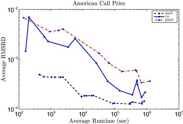
Figure 10 Runtime efficiency of American call prices with MOL, CS, and PSOR. We take the price from PSOR with a large grid consisting of ![]() time steps,
time steps, ![]() variance steps, and
variance steps, and ![]() share price steps as the true solution. The root mean-square relative differences (RMSRDs) for each method in relation to this true solution correspond to the cases with share prices ranging from
share price steps as the true solution. The root mean-square relative differences (RMSRDs) for each method in relation to this true solution correspond to the cases with share prices ranging from ![]() to
to ![]() for
for ![]() and
and ![]() .
.
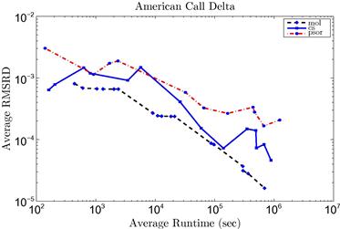
Figure 11 Runtime efficiency of American call deltas with MOL, CS, and PSOR. We take the delta from the MOL with a large grid consisting of ![]() time steps,
time steps, ![]() variance steps, and
variance steps, and ![]() share price steps as the true delta. The root mean-square relative differences (RMSRDs) for each method in relation to this true solution correspond to the cases with share prices ranging from
share price steps as the true delta. The root mean-square relative differences (RMSRDs) for each method in relation to this true solution correspond to the cases with share prices ranging from ![]() to
to ![]() for
for ![]() and
and ![]() .
.
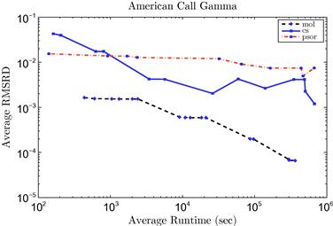
Figure 12 Runtime efficiency of gammas with MOL, CS, and PSOR. We take the American call gammas from the MOL with a large grid consisting of ![]() time steps,
time steps, ![]() variance steps, and
variance steps, and ![]() share price steps as the true gamma. The root mean-square relative differences (RMSRDs) for each method in relation to this true solution correspond to the cases with share prices ranging from
share price steps as the true gamma. The root mean-square relative differences (RMSRDs) for each method in relation to this true solution correspond to the cases with share prices ranging from ![]() to
to ![]() for
for ![]() and
and ![]() .
.
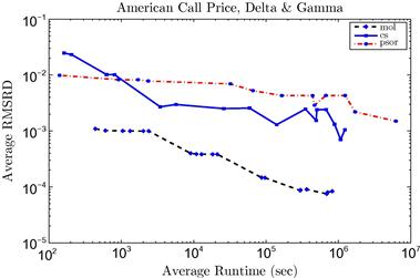
Figure 13 Overall runtime efficiency with MOL, CS, and PSOR. We take the solution from PSOR with a grid size of ![]() time steps,
time steps, ![]() variance steps, and
variance steps, and ![]() share price steps as a true solution for the price. We take the delta and gamma from the MOL with a large grid consisting of
share price steps as a true solution for the price. We take the delta and gamma from the MOL with a large grid consisting of ![]() time steps,
time steps, ![]() variance steps, and
variance steps, and ![]() share price steps as the true delta and the true gamma. The root mean-square relative differences (RMSRDs) for each method in relation to this true solution correspond to the cases with share prices ranging from
share price steps as the true delta and the true gamma. The root mean-square relative differences (RMSRDs) for each method in relation to this true solution correspond to the cases with share prices ranging from ![]() to
to ![]() and the correlations
and the correlations ![]() .
.
A number of comments based on the figures and the calculations are warranted. First, it is clear from Figure 13 that the method of lines (MOL) performs best in calculating, to similar accuracy, the call prices, deltas, and gammas. For instance, it costs MOL around 1000 s to achieve an overall relative accuracy of ![]() while it costs CS around 1,000,000 s to achieve the same overall accuracy and it takes PSOR even longer. Second, the results from the calculations (see Figures 11 and 12) show that the American call deltas and gammas seem to have a faster convergence rate than the American call prices with the MOL. This is natural because for MOL, within each iteration, the call prices are obtained after working out the deltas and gammas to the same degree of accuracy. We also see from the calculations that the value of the deltas and gammas does not change up to five decimals when refining the grid size which is also evidence indicating that the deltas and gammas with the MOL are much closer to the “true” deltas and gammas than those for both CS and PSOR.25
while it costs CS around 1,000,000 s to achieve the same overall accuracy and it takes PSOR even longer. Second, the results from the calculations (see Figures 11 and 12) show that the American call deltas and gammas seem to have a faster convergence rate than the American call prices with the MOL. This is natural because for MOL, within each iteration, the call prices are obtained after working out the deltas and gammas to the same degree of accuracy. We also see from the calculations that the value of the deltas and gammas does not change up to five decimals when refining the grid size which is also evidence indicating that the deltas and gammas with the MOL are much closer to the “true” deltas and gammas than those for both CS and PSOR.25
5 Conclusion
This paper explores the pricing of American options in the case where the underlying asset follows a jump-diffusion and stochastic volatility process. For the special case of jump-diffusion dynamics we use the approach of Jamshidian (1992) to find an inhomogeneous integro-partial differential equation (PIDE) for the American call price in an unrestricted domain, which we then solve using Fourier transforms, extending this very useful solution methodology to the jump-diffusion setting. Furthermore the approach advocated here has the advantage of being readily extended to a variety of underlying asset price dynamics, such as stochastic interest rates (see Chiarella and Kang, 2013) but using the sparse grid method, as well as handling a variety of different payoff structures, such as puts, calls, butterflies, spread options, and max-options.
We then consider the general case of both jump-diffusion and stochastic volatility dynamics and employ the method of lines to solve the integro-partial differential equation satisfied by the option price. The method of lines has the advantage that it calculates not only the price but also the delta and gamma of the option in the one calculation and to the same level of accuracy. The results are compared with those obtained using operator-splitting methods and the Crank-Nicolson method with a high degree of discretization to obtain the “exact” solution. The method of lines has been found to work quite well in the models considered here.
Future research is moving toward the sparse grid method which has been used by Chiarella and Kang (2013) to handle both stochastic interest rates and stochastic volatility dynamics. Other numerical methods have not been considered, such as the tree methods of Amin (1993) and Broadie and Yamamoto (2003), and various finite difference scheme implementations, including Andersen and Andreasen (2000) and d’Halluin et al. (2004). A detailed analysis of the relative efficiency of these various numerical methods is planned as a future research project.
References
1. Abramowitz M, Stegun IA. Handbook of Mathematical Functions. New York: Dover; 1970.
2. Adolfsson, T., Chiarella, C., Ziogas, A., Ziveyi, J., 2013. Representation and Numerical Approximation of American Option Prices Under Heston Stochastic Volatility Dynamics. Working Paper, Quantitative Finance Research Centre, University of Technology Sydney.
3. Amin KI. Jump diffusion option valuation in discrete time. Journal of Finance. 1993;48(5):1833–1863.
4. Andersen L, Andreasen J. Jump-diffusion processes: volatility smile fitting and numerical methods for option pricing. Review of Derivatives Research. 2000;4:231–262.
5. Barone-Adesi G. The saga of the American put. Journal of Banking and Finance. 2005;29:2909–2918.
6. Broadie M, Yamamoto Y. Application of the fast Gauss transform to option pricing. Management Science. 2003;49(8):1071–1088.
7. Carr P, Hirsa A. Why be backward? Forward equations for American options. Risk. 2003;16(1):103–107.
8. Carr P, Madan DB. Option valuation using the fast Fourier transform. Journal of Computational Finance. 1999;2(4):61–73.
9. Cheang G, Chiarella C, Ziogas A. The representation of American options prices under stochastic volatility and jump-diffusion dynamics. Quantitative Finance. 2013;13(2):241–253.
10. Chiarella C, Kang B. The evaluation of American compound option prices under stochastic volatility and stochastic interest rates. Journal of Computational Finance. 2013;17(1):71–92.
11. Chiarella C, Kang B, Meyer GH, Ziogas A. The evaluation of American option prices under stochastic volatility and jump-diffusion dynamics using the method of lines. International Journal of Theoretical and Applied Finance. 2009;12(3):393–425.
12. Chiarella, C., Kucera, A., Ziogas, A., 2004. A Survey of the Integral Representation of American Option Prices. Quantitative Finance Research Centre, University of Technology Sydney, Research Paper, No. 118.
13. Chiarella C, Ziogas A. Evaluation of American strangles. Journal of Economic Dynamics and Control. 2005;29:31–62.
14. Chiarella, C., Ziogas, A., 2006. A Fourier Transform Analysis of the American Call Option on Assets Driven by Jump-Diffusion Processes. Quantitative Finance Research Centre, University of Technology Sydney, Research Paper, No. 174.
15. Chiarella C, Ziogas A. American call options under jump-diffusion processes: a Fourier transform approach. Applied Mathematical Finance. 2009;16(1):37–79.
16. Clarke N, Parrott K. Multigrid for American option pricing with stochastic volatility. Applied Mathematical Finance. 1999;6:177–195.
17. Cont R, Tankov P. Financial Modelling with Jump Processes. Boca Raton, Florida: Chapman and Hall/CRC; 2003.
18. Debnath L. Integral Transforms and their Applications. Baton Rouge: CRC Press; 1995.
19. d’Halluin Y, Forsyth P, Labahn G. A penalty method for American options with jump diffusion processes. Numerische Mathematik. 2004;97:321–352.
20. Duffy DJ. Finite Difference Methods in Financial Engineering: A Partial Differential Equation Approach. Har/Cdr ed. Wiley 2006.
21. Ekstrom E, Lotstedt P, Tysk J. Boundary values and finite difference methods for the single factor term structure equation. Applied Mathematical Finance. 2009;16(3):253–259.
22. Gukhal CR. Analytical valuation of American options on jump-diffusion processes. Mathematical Finance. 2001;11:97–115.
23. Heston S. A closed-form solution for options with stochastic volatility with applications to bond and currency options. Review of Financial Studies. 1993;6:327–343.
24. Ikonen S, Toivanen J. Operator splitting methods for American options with stochastic volatility. Applied Mathematics Letters. 2004;17:809–814.
25. Ikonen S, Toivanen J. Componentwise splitting methods for pricing American options under stochastic volatility. International Journal of Theoretical and Applied Finance. 2007;10(2):331–361.
26. Jamshidian F. An analysis of American options. Review of Futures Markets. 1992;11:72–80.
27. Kallast S, Kivinukk A. Pricing and Hedging American options using approximations by kim integral equations. European Finance Review. 2003;7:361–383.
28. Kim IJ. The analytic valuation of American options. Review of Financial Studies. 1990;3:547–572.
29. Kou SG. A jump-diffusion model for option pricing. Management Science. 2002;48(8):1086–1101.
30. Kwok Y-K. Mathematical Models of Financial Derivatives. second ed. Springer 2008.
31. Lee RW. Option pricing by transform methods: extensions, unification and error control. Journal of Computational Finance. 2004;7(3):51–86.
32. Lewis AL. Option valuation under stochastic volatility. California: Finance Press; 2000.
33. McKean HP. Appendix: a free boundary value problem for the heat equation arising from a problem in mathematical economics. Industrial Management Review. 1965;6:32–39.
34. Merton RC. Option pricing when underlying stock returns are discontinuous. Journal of Financial Economics. 1976;3:125–144.
35. Meyer G. Pricing Options and Bonds with the Method of Lines. Georgia Institute of Technology 2012; In: <http://people.math.gatech.edu/meyer/MOL-notes/>; 2012.
36. Meyer GH. The numerical valuation of options with underlying jumps. Acta Mathematica. 1998;47:69–82.
37. Meyer GH, van der Hoek J. The evaluation of American options with the method of lines. Advances in Futures and Options Research. 1997;9:265–285.
38. Myneni R. The pricing of the American option. The Annals of Applied Probability. 1992;2:1–23.
39. Peskir G. On the American option problem. Mathematical Finance. 2005;15(1):169–181.
40. Pham H. Optimal stopping, free boundary, and American option in a jump-diffusion model. Applied Mathematics and Optimization. 1997;35:145–164.
41. Scott LO. Pricing stock options in a jump-diffusion model with stochastic volatility and interest rates: Applications of Fourier inversion methods. Mathematical Finance. 1997;7(4):413–426.
42. Shampine LF. Numerical Solution of Ordinary Differential Equations. New York: Chapman and Hall; 1994.
43. Strang G. On the construction and comparison of difference schemes. SIAM Journal of Numerical Analysis. 1968;5:506–517.
44. Wilmott P, Dewynne J, Howison S. Option Pricing: Mathematical Models and Computation. Oxford Financial Press 1993.
1Note that ![]() , where
, where ![]() is the maturity date of the option and
is the maturity date of the option and ![]() is current time.
is current time.
2See, for example, Cheang et al. (2012). This paper also discusses the role that the assumptions concerning the market prices of volatility risk and jump risk play in choosing a risk-neutral pricing measure ![]() .
.
3In particular the proofs of propositions 3.1–3.10.
4Pham (1997), to the authors’ knowledge, was the first to report the PIDE (15) with the inclusion of the ![]() term.
term.
5The smooth-pasting condition (21) sets the delta of the American call to be continuous at the free boundary so as to guarantee arbitrage-free prices. For the call under consideration, we note that the standard arbitrage arguments that justify condition (21) are not readily applied under Merton’s jump-diffusion model, since this depends upon the price process for ![]() being continuous. The corresponding boundary conditions were proven by Pham (1997) for the American put case, and the arguments he uses, based on the maximum principle, are readily applied to the case of the American call problem with a continuous dividend yield for
being continuous. The corresponding boundary conditions were proven by Pham (1997) for the American put case, and the arguments he uses, based on the maximum principle, are readily applied to the case of the American call problem with a continuous dividend yield for ![]() .
.
6Full details on McKean’s method applied to American calls under jump-diffusion are given by Chiarella and Ziogas (2006).
7We again refer the reader to the remark just prior to Proposition 3.1.
8Another approach, used by Cheang et al. (2012), involves applying the transform to the Kolmogorov PDE for the transition density (where the boundary conditions hold more naturally) and then using Duhamel’s principle to express the solution.
9Yet another approach would be to obtain a formal solution and then verify that it has the desired properties.
10We assume that the density function ![]() is of the form that facilitates the reduction of the
is of the form that facilitates the reduction of the ![]() -dimensional integral to a single integral. This is true of the log-normal density function that we use later.
-dimensional integral to a single integral. This is true of the log-normal density function that we use later.
11By the global variance we mean ![]() calculated from Eq. (14) to be
calculated from Eq. (14) to be ![]() in the case of a log-normal jump density.
in the case of a log-normal jump density.
12Note that the reported runtimes indicate the total time required to find the free boundary, price, and delta for the American call. Both axes are given in log-scale.
13We recall that the distribution ![]() is defined by Eq. (12).
is defined by Eq. (12).
14The Riccati transform basically replaces a given differential system (here (71) and (72)) with an equivalent set of uncoupled equations of lower dimension (here (74–76) below).
15All ODEs have been solved by use of the implicit trapezoidal rule, discussed, for example, by Shampine (1994).
16We test Eq. (77) at each grid point and find the grid points at which ![]() changes sign. We then use Newton’s method to search for the value of
changes sign. We then use Newton’s method to search for the value of ![]() by fitting a cubic spline through four points around this point.
by fitting a cubic spline through four points around this point.
17We remind the reader that at ![]() the first of the free boundary conditions (10) becomes
the first of the free boundary conditions (10) becomes ![]() .
.
18Note that ![]() is the number of
is the number of ![]() steps while
steps while ![]() and
and ![]() are the number of
are the number of ![]() steps and the number of
steps and the number of ![]() steps, respectively. This differs from other sections of the paper but we retain the original notation for ease of comparison.
steps, respectively. This differs from other sections of the paper but we retain the original notation for ease of comparison.
19In our implementation the boundary condition at ![]() is handled in the same way as those described in Section 4.1, which is different from IT.
is handled in the same way as those described in Section 4.1, which is different from IT.
20By the explicit term we mean the term on the right-hand side of each of the inequalities (90), which are at the most recent time iteration step.
21Specifically, the system of difference equations is solved using PSOR for a given estimate of the integral term. The system of difference equations is then solved again using an updated estimate for the integral term. This is repeated until the price profile converges.
22For the componentwise splitting method, the five tridiagonal systems are solved sequentially for a given estimate of the integral term. The integral term is then updated, and the tridiagonal system solved again, repeating the procedure until the price profile converges.
23RMSRD is calculated as: ![]() . It is important to use RMSRD to measure the errors from price, delta, and gamma together since they have quite different numerical scales.
. It is important to use RMSRD to measure the errors from price, delta, and gamma together since they have quite different numerical scales.
24We refer the reader to Chiarella et al. (2009) for a table with the positive correlation case, which conveys similar findings.
25Chiarella et al. (2009) also give an extended discussion of the impact of stochastic volatility and jumps on the free surface and prices. We refer the reader to this discussion as lack of space prevents us from giving these results here.
