GPU Computing in Economics
Eric M. Aldrich, Department of Economics, University of California, Santa Cruz, USA, [email protected]
Abstract
This paper discusses issues related to GPU for economic problems. It highlights new methodologies and resources that are available for solving and estimating economic models and emphasizes situations when they are useful and others where they are impractical. Two examples illustrate the different ways these GPU parallel methods can be employed to speed computation.
Keywords
Parallel computing; GPU computing; Dynamic programming; Asset pricing; Heterogeneous beliefs; General equilibrium
JEL Classification Codes
A33; C60; C63; C68; C88
1 Introduction
The first parallel computing systems date back to the 1960s and 1970s, but were limited to specialty machines with limited accessibility and distribution. Examples of early systems include the Burroughs D825 and the CDC 6600. Early development of parallel architectures led to a taxonomy of systems that defined the method by which instructions operate on data elements as well as the method of sharing memory across processing units. Two broad classifications for parallel instruction/data operation include Single-Instruction Multiple-Data (SIMD) and Multiple-Instruction Multiple-Data. In the former, SIMD, identical instructions operate on distinct data elements in a lockstep, parallel fashion. MIMD, as the name suggests, allows for more flexible design of operations across parallel data elements. These broad parallel specifications can be further dichotomized into shared and distributed memory models; shared-memory systems allowing all processor cores access to the same memory bank where the data resides, while distributed memory maintains distinct memory units for each processor (requiring movement of data elements among memory units). An overview of these architectures can be found in Dongarra and van der Steen (2012).
Advances in computational hardware and their reduction in cost led to a surge in distributed parallel computing in the 1990s. During this period, single-core microprocessor speeds were increasing at such a fast rate that powerful parallel computing systems were easily designed by connecting a large number of compute nodes, each with an individual core. Standards such as the Message Passing Interface (MPI) were developed to allow communication among the distributed nodes. The first Beowulf cluster, introduced in 1994, was an example of such a system. It is a model that has been widely utilized to the present day and which has been largely responsible for making parallel computing available to the masses. However, in the early 2000s, microprocessors became increasingly limited in terms of speed gains and much of the focus of system design in the computing industry shifted toward developing multicore and multiprocessor Central Processing Units (CPUs).
Somewhat independently, the market for high-end graphics in the entertainment industry led to the development of many-core Graphical Processing Units (GPUs) in the 1990s. These graphics cards were inherently SIMD, performing identical floating point instructions on millions of pixels, and so they were designed to have numerous individual processing units with high arithmetic intensity—many transistors dedicated to floating point, arithmetic operations, but very few dedicated to memory management and control flow. The result was that consumer-grade GPUs had high arithmetic power for a very low cost.
Some time after the turn of the millennium, a number of computational scientists, recognizing the low cost and low power consumption per unit of arithmetic power (typically measured in FLOPS—Floating Point Operations Per Second), began using GPUs as parallel hardware devices for solving scientific problems. Early examples spanned the fields of computer science (Kruger and Westermann (2002) and Purcell et al. (2002)), fluid dynamics (Harris et al. (2003)), bioinformatics (Charalambous et al. (2005)), and molecular dynamics (Stone et al. (2007)), to name a few. In each case scientists recognized similarities between their algorithms and the work of rendering millions of graphical pixels in parallel. In response to the uptake of GPU computing in broad scientific fields, NVIDIA released a set of software development tools in 2006, known as Compute Unified Device Architecture (CUDA—http://www.nvidia.com/object/cuda_home_new.html) (NVIDIA (2012a)). The intention of CUDA was to facilitate higher-level interactions with graphics cards and to make their resources accessible through industry standard languages, such as C and C++. This facilitated a new discipline of General Purpose GPU (GPGPU) computing, with a number of subsequent tools that have been developed and released by a variety of hardware and software vendors.
The uptake of GPGPU computing in Economics has been slow, despite the need for computational power in many economic problems. Recent examples include Aldrich (2011), which solves a general equilibrium asset pricing model with heterogeneous beliefs, Aldrich et al. (2011), which solves a dynamic programming problem with value function iteration, Creal (2012), which solves for the likelihood for affine stochastic volatility models, Creel and Kristensen (2011), which explores the properties of indirect likelihood estimators, Durham and Geweke (2011) and Durham and Geweke (2012), which develop a parallel algorithm for sequential Monte Carlo, Dziubinski and Grassi (2012), which replicates the work of Aldrich et al. (2011) with Microsoft’s C++Amp library (http://msdn.microsoft.com/en-us/library/vstudio/hh265137.aspx) (Microsoft (2012)), Fulop and Li (2012), which uses sequential Monte Carlo and resampling for parameter learning, and Lee et al. (2010a), which shows how to use GPUs for Markov Chain Monte Carlo and sequential Monte Carlo simulation. The objective of this paper will be to demonstrate the applicability of massively parallel computing to economic problems and to highlight situations in which it is most beneficial and of little use.
The benefits of GPGPU computing in economics will be demonstrated via two specific examples with very different structures. The first, a basic dynamic programming problem solved with value function iteration, provides a simple framework to demonstrate the parallel nature of many problems and how their computational structure can be quickly adapted to a massively parallel framework. The second example, a general equilibrium asset pricing model with heterogeneous beliefs, uses an iterative procedure to compute optimal consumption allocations for a finite time horizon ![]() . This example experiences great gains from GPU parallelism, with the GPU allowing the solution of far longer time horizons than would be feasible on a CPU. A substantial portion of this paper will also be dedicated to introducing specific hardware and software platforms that are useful for GPGPU computing, with the end objective to help researchers in economics to not only become familiar with the requisite computing tools, but also to design and adapt algorithms for use on GPU parallel hardware.
. This example experiences great gains from GPU parallelism, with the GPU allowing the solution of far longer time horizons than would be feasible on a CPU. A substantial portion of this paper will also be dedicated to introducing specific hardware and software platforms that are useful for GPGPU computing, with the end objective to help researchers in economics to not only become familiar with the requisite computing tools, but also to design and adapt algorithms for use on GPU parallel hardware.
The structure of this paper will be as follows. Section 2 will introduce the basic concepts of GPGPU computing and Section 3 will illustrate these concepts in the context of a very simple example. Sections 4 and 5 will consider the dynamic programming and heterogeneous beliefs examples mentioned above, demonstrate how the solutions can be parallelized, and report timing results. Section 6 will discuss recent developments in parallel computing and will offer a glimpse of the future of the discipline and potential changes for economic computing. Section 7 will conclude.
2 Basics of GPGPU Computing
This section will introduce the basics of GPU hardware, software, and algorithms. The details of this section will be useful for understanding the specific applications in Sections 3–5.
2.1 Hardware Architecture
Understanding the basics of GPU architecture facilitates the design of massively parallel software for graphics devices. For illustrative purposes, this section will often reference the specifications of an NVIDIA Tesla C2075 GPU (NVIDIA (2011)), a current high-end GPU intended for scientific computing.
2.1.1 Processing Hardware
GPUs are comprised of dozens to thousands of individual processing cores. These cores, known as thread processors, are typically grouped together into several distinct multiprocessors. For example, the Tesla C2075 has a total of 448 cores, aggregated into groups of 32 cores per multiprocessor, yielding a total of 14 multiprocessors. Relative to CPU cores, GPU cores typically:
• Have a lower clock speed. Each Tesla C2075 core clocks in at 1.15 GHz, which is roughly 30–40% the clock seed of current CPUs (e.g., the current fastest desktop and server CPUs made by Intel are the 3.6 GHz i7-3820 (Intel Corporation (2013a)) and the 2.67 GHz E7-8837 (Intel Corporation (2011)), respectively).
• Dedicate more transistors to arithmetic operations and fewer to control flow and data caching.
• Have access to less memory. A Tesla C2075 has 6 gigabytes of global memory, shared among all cores.
Clearly, where GPU cores are lacking in clock speed and memory access, they compensate with the sheer quantity of compute cores. For this reason, they are ideal for computational work that has a high arithmetic intensity: many arithmetic operations for each byte of memory transfer/access. It is important to note that this does not mean that every problem which requires high arithmetic intensity will benefit from GPU parallelization; in addition to arithmetic intensity, the problem must be divisible into hundreds or thousands of data elements, each requiring an almost identical sequence of computational operations. Where these latter conditions are not met, a heterogeneous CPU environment, using OpenMP or MPI, may be ideal.
Figure 1 depicts a schematic diagram of CPU and GPU architectures, taken from Section 1.1 of NVIDIA (2012a). The diagram illustrates the allocation of transistors for each type of microprocessor. In particular, traditional CPUs dedicate relatively more transistors to memory and control flow (the yellow and orange blocks) and fewer to algorithmic logic units (ALUs) which perform floating point computations (the green blocks). GPUs, on the other hand, dedicate many more transistors to ALUs and far fewer to memory and control.
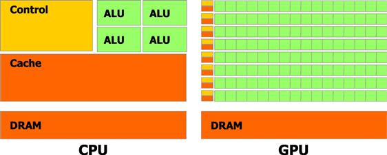
Figure 1 Schematic diagram of CPU and GPU processors, taken from Section 1.1 of NVIDIA (2012a). The diagram illustrates how traditional CPUs dedicate more transistors to memory and control (yellow and orange blocks) and fewer to floating point operations (green blocks), relative to GPUs. (For interpretation of the references to color in this figure legend, the reader is referred to the web version of this book.)
2.1.2 Memory
There is a distinction between CPU memory and GPU memory, the former being referred to as “host” memory and the latter as “device” memory. GPU instructions can only operate on data objects that are located in device memory—attempting to pass a variable in host memory as an argument to a kernel would generate an error. Thus, GPU software design often necessitates the transfer of data objects between host and device memory.
Currently, memory transfers between host and device occur over a PCIe v2.0 ![]() interface, which for an NVIDIA Tesla C2075 GPU translates into a maximum data transfer bandwidth of 8 gigabytes per second (PCI-SIG (2006)). This is approximately 1/4th the bandwidth between common configurations of host memory and CPU at the present date. For this reason it is crucial to keep track of host-device memory transfers, since programs that require large amounts of CPU-GPU data transfer relative to the number of floating point operations performed by the GPU can experience severe limits to performance.
interface, which for an NVIDIA Tesla C2075 GPU translates into a maximum data transfer bandwidth of 8 gigabytes per second (PCI-SIG (2006)). This is approximately 1/4th the bandwidth between common configurations of host memory and CPU at the present date. For this reason it is crucial to keep track of host-device memory transfers, since programs that require large amounts of CPU-GPU data transfer relative to the number of floating point operations performed by the GPU can experience severe limits to performance.
The architecture of GPU memory itself is also important. While all GPU cores share a bank of global memory, portions of the global memory are partitioned for shared use among cores on a multiprocessor. Access to this shared memory is much faster than global memory. While these issues can be beneficial to the design of parallel algorithms, the intricacies of GPU memory architecture are beyond the scope of this paper. A detailed treatment of GPU memory architecture and use can be found in NVIDIA (2012a).
2.1.3 Scaling
Two notions of scalability are relevant to GPU computing: scaling within GPU devices and across GPU devices. One powerful feature of GPU computing is that it automatically handles within-device scaling when software is moved to GPU devices with differing numbers of cores. GPU interfaces (discussed below) allow software designers to be agnostic about the exact architecture of a stand-alone GPU—the user does nothing more than designate the size of thread blocks (described in Section 2.2), which are then allocated to multiprocessors by the GPU scheduler. Although different block sizes are optimal for different GPUs (based on number of processing cores), it is not requisite to change block sizes when moving code from one device to another. The upshot is that the scheduler deals with scalability so that issues related to core count and interaction among cores on a specific device are transparent to the user. This increases the portability of massively parallel GPU software.
GPU occupancy is a measure of the number of threads concurrently scheduled on an individual core and is related to within-GPU scaling. While the number of total threads can be less than the number of cores, GPU devices achieve their best performance results when there are many threads concurrently scheduled on each core. Each device has a limit (which varies by device) to the number of threads which can be scheduled on a multiprocessor and occupancy is the ratio of actual scheduled thread warps (defined below) to the maximum number possible (NVIDIA (2012a)).
Scalability across GPU devices is achieved in a more traditional manner, using OpenMP or MPI.
2.2 Algorithmic Design
For a given computational program, there is no guarantee that any portion of the program may be computed in parallel. In practice, most algorithms have some fraction of instructions which must be performed sequentially, and a remaining fraction which may be implemented in parallel. Amdahl’s Law (Amdahl (1967)) states that if a fraction ![]() of a program can be executed in parallel, the theoretical maximum speedup of the program with
of a program can be executed in parallel, the theoretical maximum speedup of the program with ![]() processing cores is
processing cores is
![]() (1)
(1)
The intuition behind Amdahl’s Law is the following. If a serial version of an algorithm takes 1 unit of time to execute, a fraction ![]() of a parallel algorithm will execute in the same time as its serial counterpart, whereas a fraction
of a parallel algorithm will execute in the same time as its serial counterpart, whereas a fraction ![]() will run in
will run in ![]() units of time (because it can be run in parallel on
units of time (because it can be run in parallel on ![]() cores). Dividing 1 unit of time by the parallel compute time yields the possible speedup in Eq. (1). A crucial step in GPU computing is determining which portion of an algorithm can be executed in parallel.
cores). Dividing 1 unit of time by the parallel compute time yields the possible speedup in Eq. (1). A crucial step in GPU computing is determining which portion of an algorithm can be executed in parallel.
Kernels and threads are the fundamental elements of GPU computing problems. Kernels are special functions that comprise a sequence of instructions that are issued in parallel over a user specified data structure (e.g., the fraction of instructions ![]() mentioned above, such as performing a routine on each element of a vector). Thus, a kernel typically comprises only a portion of the total set of instructions within an algorithm. Each data element and corresponding kernel comprise a thread, which is an independent problem that is assigned to one GPU core.
mentioned above, such as performing a routine on each element of a vector). Thus, a kernel typically comprises only a portion of the total set of instructions within an algorithm. Each data element and corresponding kernel comprise a thread, which is an independent problem that is assigned to one GPU core.
Just as GPU cores are grouped together as multiprocessors, threads are grouped together in user-defined groups known as blocks. Thread blocks execute on exactly one multiprocessor, and typically many thread blocks are simultaneously assigned to the same multiprocessor. A diagram of this architecture is depicted in Figure 2, taken from Section 1.1 of NVIDIA (2012a). The scheduler on the multiprocessor then divides the user-defined blocks into smaller groups of threads that correspond to the number of cores on the multiprocessor. These smaller groups of threads are known as warps — as described in NVIDIA (2012a), “The term warp originates from weaving, the first parallel thread technology.” As mentioned above, each core of the multiprocessor then operates on a single thread in a warp, issuing each of the kernel instructions in parallel. This architecture is known as Single-Instruction Multiple-Thread (SIMT) (NVIDIA (2012a)).
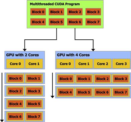
Figure 2 Schematic diagram of thread blocks and GPU multiprocessors, taken from Section 1.1 of NVIDIA (2012a). This diagram shows how (1) each thread block executes on exactly one GPU multiprocessor and (2) multiple thread blocks can be scheduled on the same multiprocessor.
Because GPUs employ SIMT architecture, it is important to avoid branch divergence among threads. While individual cores operate on individual threads, the parallel structure achieves the greatest efficiency when all cores execute the same instruction at the same time. Branching within threads is allowed, but asynchronicity may result in sequential execution over data elements of the warp. Given the specifications of GPU cores, sequential execution would be horribly inefficient relative to simply performing sequential execution on the CPU.
2.3 Software
NVIDIA was the original leader in developing a set of software tools allowing scientists to access GPUs. The CUDA C language (NVIDIA (2012a)) is simply a set of functions that can be called within basic C/C++ code that allow users to interact with GPU memory and processing cores. CUDA C is currently the most efficient and best documented way to design GPU software — it is truly the state of the art. Downsides to CUDA C are that it requires low-level comfort with software design (similar to C/C++) and that it only runs on NVIDIA GPUs running the CUDA platform. The CUDA platform itself is free, but requires NVIDIA hardware. While originally designed only for C/C++, it is now possible to write CUDA C kernels for Fortran, Python, and Java.
OpenCL (http://www.khronos.org/opencl/) is an open source initiative led by Apple and promoted by the Khronos Group. The syntax of OpenCL is very similar to CUDA C, but it has the advantage of not being hardware dependent. In fact, not only can OpenCL run on a variety of GPUs (including NVIDIA GPUs), it is intended to exploit the heterogeneous processing resources of differing GPUs and CPUs simultaneously within one system. The downside to OpenCL is that it is poorly documented and has much less community support than CUDA C. In contrast to NVIDIA CUDA, it is currently very difficult to find a cohesive set of documentation that assists an average user in making a computer system capable of running OpenCL (e.g., downloading drivers for a GPU) and in beginning the process or software design with OpenCL.
Beyond these two foundational GPU software tools, more and more third-party vendors are developing new tools, or adding GPU functionality within current software. Examples include the Parallel Computing Toolbox in Matlab and the CUDALink and OpenCLLink interfaces in Mathematica. New vendors, such as AccelerEyes (http://www.accelereyes.com/) are developing libraries that allow higher-level interaction with the GPU: their Jacket product is supposed to be a superior parallel computing library for Matlab, and their ArrayFire product is a matrix library that allows similar high-level interaction within C, C++, and Fortran code. ArrayFire works with both the CUDA and OpenCL platforms (i.e., any GPU) and the basic version is free. For a licensing fee, users can also gain access to linear algebra and sparse grid library functions.
Similar to ArrayFire, matrix libraries such as Thrust, ViennaCL, and C++Amp have been developed to allow higher-level GPU support within the context of the C and C++ languages. All are free, although each has specific limitations: e.g., Thrust only works on the CUDA platform, and, at present, C++Amp only works on the Windows operating system via Visual Studio 2012 (and hence is not free if VS2012 cannot be obtained through an academic license). While tied to NVIDIA hardware, Thrust is a well-documented and well-supported library which will be featured below.
One of the limitations of GPU computing relative to parallel computing with traditional CPUs is that there are fewer software tools available. Further, those which are available tend to be less sophisticated. Debugging software and numerical libraries are examples—in particular, far fewer numerical libraries are currently available for GPU than CPU computing. However, given the rapid uptake of GPUs for scientific computing, this will most likely change in the near future (as evidenced by the discussion of dynamic parallelism and GPU callable libraries in Section 6.1).
3 A Simple GPGPU Example
Let us now turn to a simple problem that can be computed with a GPU and illustrate how it can be implemented in several computing languages. One of the primary objectives of this section will be to provide demonstration code that can serve as a template for using GPUs in economic research and which will serve as a foundation for understanding the applications in Sections 4 and 5.
Consider the second-order polynomial
![]() (2)
(2)
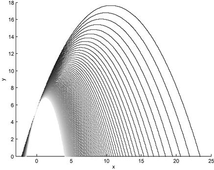
Suppose that we wish to optimize the polynomial for a finite set of values of the second-order coefficient in a specific range: ![]() . Figure 3 depicts this range of polynomials when
. Figure 3 depicts this range of polynomials when ![]() and
and ![]() , and where the darkest line corresponds to the case
, and where the darkest line corresponds to the case ![]() . In this example it is trivial to determine the location of the optimum,
. In this example it is trivial to determine the location of the optimum,
![]() (3)
(3)
However, to illustrate the mechanics of parallel computing we will compute the solution numerically with Newton’s Method for each ![]() .
.
The remainder of this section will show how to solve this problem with Matlab, C++, CUDA C, and Thrust.1 The Matlab and C++ codes are provided merely as building blocks—they are not parallel implementations of the problem. In particular, the Matlab code serves as a baseline and demonstrates how to quickly solve the problem in a language that is familiar to most economists. The C++ code then demonstrates how easily the solution can be translated from Matlab to C++; indeed, most economists will be surprised at the similarity of the two languages. Finally, understanding the serial C++ implementation is valuable for CUDA C and Thrust, since these latter implementations are simply libraries that extend the C++ framework.
3.1 Matlab
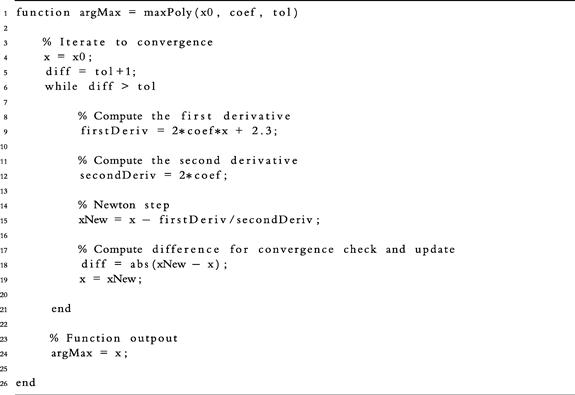
Listing 1 displays the file main.m, which solves the optimization problem above for various values of the second-order coefficient. The block of code on lines 2–4
constructs a grid, paramGrid, of nParam = 1000 values between ![]() and
and ![]() . Line 8 then allocates a vector for storing the arg max values of the polynomial at each
. Line 8 then allocates a vector for storing the arg max values of the polynomial at each ![]() ,
,
and lines 9–11 loop over each value of paramGrid and maximize the polynomial by calling the function maxPoly,
To numerically solve for the maximum at line 10, Matlab provides built-in optimization functions such as fmincon; alternatively, superior third-party software, such as KNITRO (http://www.ziena.com/knitro.htm), could be used. To keep the Matlab software similar to the implementations below, we make use of a self-written Newton solver wrapped in the function maxPoly, which is shown in Listing 2. The first line of the listing
shows that maxPoly accepts three arguments: an initial value for ![]() , x0, a value of the second-order coefficient, coef, and a convergence tolerance, tol. On exit, the function returns a single value, argMax, which is the arg max of the function. Lines 4 and 5
, x0, a value of the second-order coefficient, coef, and a convergence tolerance, tol. On exit, the function returns a single value, argMax, which is the arg max of the function. Lines 4 and 5
initialize the arg max, ![]() , and create a variable, diff, which tracks the difference between Newton iterates of
, and create a variable, diff, which tracks the difference between Newton iterates of ![]() . The main Newton step then occurs within the while loop between lines 6 and 21. In particular, lines 9 and 12 compute the first and second derivatives of the polynomial,
. The main Newton step then occurs within the while loop between lines 6 and 21. In particular, lines 9 and 12 compute the first and second derivatives of the polynomial,
and line 15
uses the derivatives to update the value of the arg max, xNew. Each iteration terminates by computing the difference between the new and current iterates
and then setting the new value of the arg max to be the current value
When convergence is achieved (diff < tol ), the function exits and returns the most recent value of ![]() . As is seen above, the basic nature of the problem makes it very easy to solve with few lines of code.
. As is seen above, the basic nature of the problem makes it very easy to solve with few lines of code.
3.2 C++
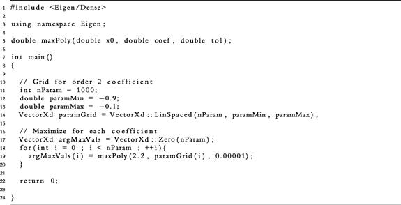
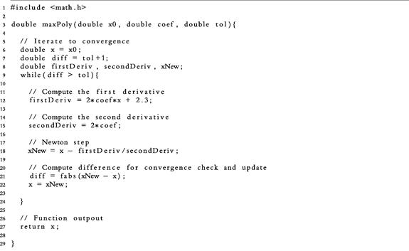
Listings 3 and 4 display C++ code for the polynomial optimization problem. This code makes no direct advances toward parallelization, but sets the framework for subsequent parallel implementations (CUDA C and Thrust) which build on C++. While most economists are not comfortable with C++, many will be surprised by the similarity between the Matlab and C++ code, especially the functions maxPoly.m and maxPoly.cpp.
Listing 3 shows the file main.cpp which corresponds to the Matlab script main.m in Listing 1. Two general notes about C++ syntax will be beneficial:
1. Single-line comments in C++ begin with //, as opposed to % in Matlab. Multiline comments begin with /* and end with */.
2. Functions and conditional statements in C++ begin and end with curly braces {}, whereas in Matlab only the end point is explicitly defined with the statement end.
The first notable difference between main.cpp and main.m arises in lines 1 and 3 of the former,
where the Eigen library is called: Eigen (http://eigen.tuxfamily.org) is a template library that provides basic linear algebra functionality. By default, C++ does not load many of the basic libraries that are beneficial for scientific computing—these must be invoked explicitly in the software.
The next difference is the declaration of the function maxPoly in line 5
Before any variable or function can be used in C++, it must be declared and initialized. Further, declarations require a statement of type: in this case the double preceding the name of the function states that the function will return a double precision variable, and the instances of double before each of the function arguments also state that the arguments will be double precision values. The function itself is only declared in main.cpp and not defined—the definition is fully enclosed in maxPoly.cpp. However, in order to utilize the function, main.cpp must have access to the definition of maxPoly and not only its declaration. This is accomplished by linking the two C++ files at compile time, which can either be done on the command line or in a separate makefile, a topic which is beyond the scope of this paper. To see how this is accomplished in a makefile, readers can download code for this example at http://www.parallelecon.com/basic-gpu/.
Unlike Matlab, which allows users to write an interactive script, all C++ code must be wrapped in an outer function entitled main. This is seen in line 7 of Listing 3. Convention is that main returns an integer value: 0 if the program is successful, 1 otherwise. Within the main function, we see the same operations being performed as in main.m. First, the grid of second-order coefficients, paramGrid, is constructed
Clearly, nParam is declared to be an integer and paramMin and paramMax are double precision. Less obviously, paramGrid is declared as type VectorXd, which is a double precision vector made available by Eigen. The function LinSpaced(n,a,b) constructs an equally spaced array of n values between a and b.
VectorXd argMaxVals = VectorXd::Zero(nParam);
for(int i = 0 ; i < nParam ; ++i){
then allocate storage for the arg max values and loop over paramGrid, performing the maximization by calling maxPoly for each value of the grid. Aside from previously mentioned syntactical differences, these lines are identical to their Matlab counterpart. Listings 2 and 4 show that the same is true of the functions maxPoly.m and maxPoly.cpp: aside from previously mentioned syntactical differences and line 1 of main.cpp
which explicitly invokes the basic math library math.h, these two files are essentially identical.
3.3 CUDA C
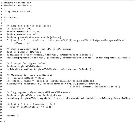
CUDA C is a set of C/C++ callable functions that provide an interface to NVIDIA graphics devices. Listings 5 and 6 display parallel GPU code, written in C++, making use of CUDA C function calls. Note that the file name extensions have been changed from .cpp to .cu. The first line of Listing 5
serves the purpose of declaring and defining the function in maxPoly.cu. Lines 7-9 of Listing 5 show that nParam, paramMin, and paramMax are declared and initialized exactly as in main.cpp, however the initialization of paramGrid on lines 10 and 11 is somewhat different:
Where the C++ code declared paramGrid to be an Eigen vector of double precision values and initialized the grid with the function LinSpaced, the CUDA C implementation is a bit more rudimentary: it declares a basic C array on line 10 and then initializes each value of the array with a for loop. The reason for this is that the CUDA compiler, nvcc, does not support the object-oriented functionality of the Eigen library and hence cannot compile CUDA code with Eigen references.
One of the major differences between main.cpp and main.cu centers on the use of host and device memory (discussed in Section 2.1.2): in order to maximize the polynomial for each value of paramGrid on the GPU, the grid must first be declared and initialized in host memory, as on lines 10 and 11 of Listing 5, and then transferred to device memory. The transfer is accomplished in two steps. First, on lines 14 and 15
memory is explicitly allocated on the device. The essential features are that line 14 declares a new double precision vector paramGridDevice (in reality, the asterisk states that paramGridDevice is a “pointer” that points to a block of memory that has been set aside for double precision variables) and line 15 allocates enough space in memory for nParam double precision variables. The second step on line 16
uses the function cudaMemcpy to explicitly copy the variable paramGrid in host memory to the empty vector paramGridDevice in device memory. Similar syntax is used to declare and initialize a vector argMaxValsDevice on lines 19 and 20, but since the initial values are unimportant there is no need to explicitly copy predefined values from host to device memory. Only after the optimization has been performed, with the arg max values stored in argMaxValsDevice, does the code return the solution to host memory on lines 29 and 30
Note that to complete the transfer, the variable argMaxVals must first be declared and initialized in host memory, since this was not done previously.
The final, crucial difference between Listings 3 and 5 occurs at lines 23–25, where the loop over paramGrid has been eliminated and replaced with a CUDA C call to the kernel maxPoly:
int blocksPerGrid = (int)ceil((double)nParam/threadsPerBlock);
maxPoly <<<blocksPerGrid, threadsPerBlock>>>(2.2, paramGridDevice,
The <<<x,y>>> syntax is the core CUDA C interface to request parallel operation on a data structure. The first argument can either be an integer or a one-, two-, or three-dimensional object of type dim3, which specifies the dimensions of the grid containing thread blocks (i.e., the thread blocks can be arranged in an array structure of up to three dimensions). If this argument is an integer scalar ![]() , the grid is one-dimensional with
, the grid is one-dimensional with ![]() elements (i.e.,
elements (i.e., ![]() thread blocks). The second argument is either an integer or a one- or two-dimensional object of type dim3 which specifies the dimensions of a thread block. In the example above, <<<blocksPerGrid, threadsPerBlock>>> specifies a one-dimensional grid containing
thread blocks). The second argument is either an integer or a one- or two-dimensional object of type dim3 which specifies the dimensions of a thread block. In the example above, <<<blocksPerGrid, threadsPerBlock>>> specifies a one-dimensional grid containing ![]() one-dimensional thread blocks of
one-dimensional thread blocks of ![]() threads. Note that the syntax on line 24
threads. Note that the syntax on line 24
ensures that there are always enough thread blocks in the grid to contain all of the nParam threads by rounding the value nParam/threadsPerBlock up to the nearest integer (the use of (double) and (int) force all variables to be cast as the right types). The upshot is that line 25 requests the operations in the kernel maxPoly to be performed in parallel on blocks of 256 elements of paramGridDevice. It is important to note that while different block sizes are optimal for different GPUs (depending on the number of cores), this variable defines the number of threads per block and is independent of the total number of GPU cores (i.e., it does not need to be changed when moving the code from one GPU to another—even if a GPU has fewer than 256 cores).
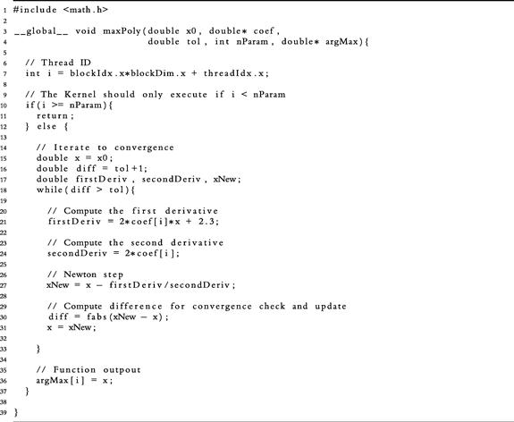
The C++ function maxPoly.cpp and CUDA kernel maxPoly.cu are almost exactly identical. The first difference occurs in the kernel definition on line 3 of Listing 6:
The following is a breakdown of the how this line differs from the corresponding definition in maxPoly.cpp:
• _ _global_ _ is CUDA C syntax for declaring a kernel (referring to global device memory).
• The kernel must return type void, which is true of all CUDA kernels (as compared to the double return type of maxPoly.cpp). This means that maxPoly.cu returns nothing.
• The second argument of the kernel is the full vector (in reality, a pointer to the vector in memory) of possible second-order coefficients, rather than a single element of the coefficient array.
• The kernel has an additional argument, nParam, which is the integer length of the coefficient vector, coef.
• Because it returns void, the kernel has been augmented with an additional argument, argMax, which is an empty vector where the solutions are stored. In particular, since a pointer to the location of the vector in memory is passed (the * notation) the values can be modified by the function and will remain modified upon exit.
is the operative line of code that CUDA uses to assign data elements to processor threads. Within a particular kernel, the values blockIdx.x, blockIdx.y, and blockIdx.z correspond to the three-dimensional indices of a unique block within the grid of blocks and the values threadIdx.x and threadIdx.y are the two-dimensional indices of a unique thread within a block. Variables blockDim.x and blockDim.y correspond to the number of threads along each dimension of a block. Coupling block indices with block dimensions traverses the threads within the grid to select the initial thread element of a block within the grid. In this example, with a total of 4 blocks, ![]() (indexing in C++ begins at zero), blockDim.x = 256 and
(indexing in C++ begins at zero), blockDim.x = 256 and ![]() . Hence, the variable i corresponds to a unique element in the parameter grid coef, which is used on lines 21 and 24 and which results in a final solution, argMax, on line 36. The commands
. Hence, the variable i corresponds to a unique element in the parameter grid coef, which is used on lines 21 and 24 and which results in a final solution, argMax, on line 36. The commands
on lines 10–12 ensure that the kernel only operates on array indices that are less than nParam. If the number of data elements is not perfectly divisible by the block size, the grid of blocks will contain thread elements which exceed the number of threads needed for computation—that is, the use of ceil in the code causes the number of threads in the grid of blocks to be at least as great as nParam. In the example above, the grid of blocks has 1024 threads, whereas the coefficient vector only has 1000 elements. Without the conditional statement above, kernels will operate on threads that exceed nParam, potentially altering values in memory that are reserved for computations by other multiprocessors. Hence, lines 10–12 serve as a protection for memory objects that do not belong to the coefficient vector coef.
In summary, this code allows the CUDA runtime environment to divide thread blocks among available multiprocessors, which then schedules individual threads to individual cores. As emphasized above, the scheduling of blocks is transparent to the user and scales automatically to the number of multiprocessors. Each thread process then accesses a unique ID in the thread block via the threadIdx command. The end result is that the sequential loop is eliminated and each GPU core is able to issue the kernel instructions for optimization in parallel on individual elements of the parameter vector. Because of transparent scaling, this code can run on a laptop with only 32 GPU cores or on a Tesla C2075 with 448 cores without modification.
3.4 Thrust
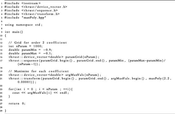
As mentioned above, Thrust is a free template library that can be called within C/C++ and which provides an alternate interface to GPU hardware. Listings 7 and 8 display parallel GPU code written in C++, making use of the Thrust template library. The primary advantage of Thrust is that it combines the conciseness of Matlab and C++/Eigen code with the ability to schedule parallel work on a GPU. In particular, Thrust eliminates the need for explicit memory allocation and transfer between host and device. Although the transfer must still occur, allocating and copying a data object in device memory is as simple as
double* Y = new double[N]; // Allocate a vector, Y, of N elements in host memory
thrust::device_vector<double> X = Y; // Allocate and copy to device memory
in contrast to the excessively verbose use of cudaMalloc and cudaMemcpy in CUDAC. This greatly facilitates the development of software as it allows the user to work at a high level of abstraction, without the need to deal with the minor details of memory allocation and transfer.
Lines 1–3 of Listing 7 include the relevant Thrust libraries for use in C++ and line 4
is the equivalent of including the maxPoly kernel source code, which will be described below. The declarations of nParam, paramMin, and paramMax on lines 10–12 are identical to those in C++ and CUDA C, so the first major difference arises on lines 13 and 14 with the declaration and initialization of paramGrid:
thrust::device_vector<double> paramGrid(nParam);
The syntax thrust::device_vector instantiates a vector directly in device memory. The function thrust::sequence(start, end, lower, step) then constructs an equally spaced sequence of points between the positions start and end of a Thrust vector, beginning at the value lower, with the grid points step units apart. Unlike CUDA C, where paramGrid first had to be computed in host memory and transferred to device memory, we see that Thrust allows functionality to build such a grid directly in the device memory. This not only saves time in transferring data, but also results in more streamlined code.
Line 17 then declares and allocates memory for a device vector, argMaxVals, which is not transferred to host memory at the end of the program because Thrust allows users to access and manipulate members of a device vector as if they reside in host memory. The important parallel operation of the file occurs at line 18:
In contrast to the <<<x,y>>> syntax of CUDA C, the parallel interface in Thrust is provided by two functions: thrust::transform and thrust::for_each. Specifically,
applies function to each element of a Thrust vector between inputStart and inputEnd and places the output in the Thrust vector starting at outputStart. Although it is not described here, thrust::for_each provides similar functionality. Most users find this interface to be a bit more intuitive than that of CUDA C.
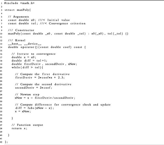
While we previously saw that the files maxPoly.m, maxPoly.cpp, and maxPoly.cu were almost identical, a brief glance at Listing 8 shows substantial differences in the Thrust equivalent, maxPoly.hpp (which is referred to as a “functor” or function object). The major differences arise from the fact that Thrust encloses the “kernel” in a C++ class structure rather than in a simple function. Line 3
is the C/C++ syntax for declaring such an object and Lines 6, 7, and 10
const double x0; ///< Initial value
const double tol; ///< Convergence criterion
maxPoly(const double _x0, const double _tol) : x0(_x0), tol(_tol) {}
declare the members of the object. In this case, the members are the actual function maxPoly and the arguments to the function (the initial value of the arg max, x0, and the Newton convergence tolerance, tol). Lines 13 and 14
provide the syntax for an operator (), which is the object interface for maxPoly, and the instructions between lines 14 and 35 are identical to those found in maxPoly.cpp. Note that there is no explicit use of a thread ID in Thrust, nor does maxPoly take paramGrid as an argument—these details are handled transparently via thrust::transform. Also, where users must specify a thread block structure in CUDA C, Thrust handles details of blocks and grids under the hood.
The final advantage of Thrust is that it has separate backends for CUDA and OpenMP; that is, the same software can access GPU or shared-memory CPU parallelism (although not both at the same time). The result is that Thrust software can run without modification on systems that do not have GPU capabilities, but that have multiple CPUs cores that share memory. This will be demonstrated in the examples of the following sections. For more details on using the Thrust interface, see Bell and Hoberock (2012) or the Thrust Quickstart Guide (NVIDIA (2012b)).
4 Example: Value Function Iteration
We will now turn our attention to a specific example where parallelism can greatly speed up the computation of an economic model. Specifically, we will consider a canonical real business cycle (RBC) model (Kydland and Prescott (1982)) solved with value function iteration (VFI) (Judd (1998)). While this model is simple, it is an excellent illustration of the benefits of a parallel architecture. The results of this section are based upon those of Aldrich et al. (2011) with some minor modifications and code to replicate the results is available at http://www.parallelecon.com/vfi/.
4.1 Model
The economy is populated by a representative agent with preferences over a single consumption good. The agent seeks to maximize expected lifetime utility,
 (4)
(4)
where ![]() is the agent’s consumption at time
is the agent’s consumption at time ![]() is the conditional expectations operator at
is the conditional expectations operator at ![]() , and
, and ![]() is the discount factor. For this example we specialize the period utility function to be of the constant relative risk aversion form:
is the discount factor. For this example we specialize the period utility function to be of the constant relative risk aversion form:
![]() (5)
(5)
where ![]() is the coefficient of relative risk aversion.
is the coefficient of relative risk aversion.
The agent receives income each period by renting labor and capital to a representative firm and chooses consumption and investment so as to satisfy the budget constraints
![]() (6)
(6)
where ![]() is the wage paid for a unit of labor,
is the wage paid for a unit of labor, ![]() is the rental rate for a unit of capital,
is the rental rate for a unit of capital, ![]() is capital,
is capital, ![]() is investment, and where we have assumed that labor,
is investment, and where we have assumed that labor, ![]() , is normalized to unity and supplied inelastically because it does not enter the agent’s utility function. Capital depreciates each period according to
, is normalized to unity and supplied inelastically because it does not enter the agent’s utility function. Capital depreciates each period according to
![]() (7)
(7)
where ![]() is the depreciation rate.
is the depreciation rate.
The representative firm produces output according to
![]() (8)
(8)
where ![]() is output and where the total factor of productivity (TFP),
is output and where the total factor of productivity (TFP), ![]() , follows the law of motion
, follows the law of motion
![]() (9)
(9)
We will assume that the production function is of the Cobb-Douglas form:
![]() (10)
(10)
where ![]() is the output elasticity of capital. Combining Eqs. (6)–(8) with the market clearing condition
is the output elasticity of capital. Combining Eqs. (6)–(8) with the market clearing condition ![]() , we arrive at the aggregate resource constraint
, we arrive at the aggregate resource constraint
![]() (11)
(11)
Since the welfare theorems are satisfied, we can find the agent’s optimal consumption path by solving a recursive version of a social planner’s problem
 (12a)
(12a)
subject to
![]() (12b)
(12b)
![]() (12c)
(12c)
where the recursive structure of the problem allows us to simplify notation by dropping time subscripts: a variable ![]() refers to its value in the current time period, while
refers to its value in the current time period, while ![]() denotes its value in the subsequent period. It is not requisite to solve the model with VFI in order to achieve the advantages of massive parallelism—we could obtain similar benefits by working directly with the equilibrium conditions. However, the problem is most easily illustrated in the present format.
denotes its value in the subsequent period. It is not requisite to solve the model with VFI in order to achieve the advantages of massive parallelism—we could obtain similar benefits by working directly with the equilibrium conditions. However, the problem is most easily illustrated in the present format.
4.2 Solution
Since ![]() and
and ![]() are both continuous, strictly increasing and concave, and
are both continuous, strictly increasing and concave, and ![]() are i.i.d. shocks drawn according to a Lebesgue probability measure, Theorem 9.8 of Stokey et al. (1989) proves that System (12) has a unique functional solution
are i.i.d. shocks drawn according to a Lebesgue probability measure, Theorem 9.8 of Stokey et al. (1989) proves that System (12) has a unique functional solution ![]() and that there also exists a unique policy function,
and that there also exists a unique policy function, ![]() , for the endogenous state variable,
, for the endogenous state variable, ![]() . Unfortunately, there are no closed-form, analytical solutions for
. Unfortunately, there are no closed-form, analytical solutions for ![]() and
and ![]() , so they must be approximated numerically. Judd (1998) highlights several ways to arrive at numerical solutions for this problem, one of which is value function iteration (VFI). In brief, VFI specifies a domain
, so they must be approximated numerically. Judd (1998) highlights several ways to arrive at numerical solutions for this problem, one of which is value function iteration (VFI). In brief, VFI specifies a domain ![]() and a functional form for
and a functional form for ![]() . Discretizing the domain and starting with an initial guess,
. Discretizing the domain and starting with an initial guess, ![]() , for the value function, VFI iterates on System (12), using a numerical integration method, until successive iterates of the value function converge. Convergence for this problem is guaranteed by Theorem 9.6 of Stokey et al. (1989).
, for the value function, VFI iterates on System (12), using a numerical integration method, until successive iterates of the value function converge. Convergence for this problem is guaranteed by Theorem 9.6 of Stokey et al. (1989).
Given discretizations ![]() and
and ![]() of
of ![]() and
and ![]() , a sequential implementation of VFI would use the current iterate of the value function,
, a sequential implementation of VFI would use the current iterate of the value function, ![]() , to iterate through pairs of points in
, to iterate through pairs of points in ![]() and solve the optimization problem of System (12). The result would be an updated value function,
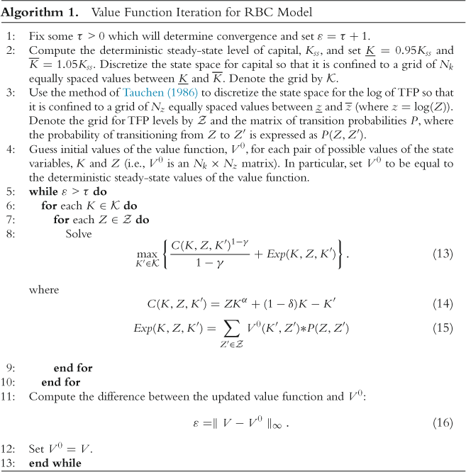
and solve the optimization problem of System (12). The result would be an updated value function, ![]() , computed in a serial fashion over each pair of state values. The algorithm would then repeat the procedure until convergence of the value function. Algorithm 1 writes the VFI computations explicitly. In summary, a serial implementation loops through the grid values in Steps 6 and 7 in sequence, performing the maximization in Eq. (13) for each pair. Note that if either
, computed in a serial fashion over each pair of state values. The algorithm would then repeat the procedure until convergence of the value function. Algorithm 1 writes the VFI computations explicitly. In summary, a serial implementation loops through the grid values in Steps 6 and 7 in sequence, performing the maximization in Eq. (13) for each pair. Note that if either ![]() or
or ![]() is a very dense grid, Step 8 may involve many thousands of serial calculations for each of the values in the loops at Steps 6 and 7.
is a very dense grid, Step 8 may involve many thousands of serial calculations for each of the values in the loops at Steps 6 and 7.
Alternatively, with many processing cores available, the maximization problems computed for each ![]() pair could be assigned to individual cores and computed in parallel. In Algorithm 1 this amounts to eliminating the loops in Steps 6 and 7 and outsourcing the computations of Eq. (13) to multiple cores. The reason that parallelism can be exploited in this problem is that the maximization nested within Steps 6 and 7 depends only on the concurrent
pair could be assigned to individual cores and computed in parallel. In Algorithm 1 this amounts to eliminating the loops in Steps 6 and 7 and outsourcing the computations of Eq. (13) to multiple cores. The reason that parallelism can be exploited in this problem is that the maximization nested within Steps 6 and 7 depends only on the concurrent ![]() and not on other values in
and not on other values in ![]() and
and ![]() . Aldrich et al. (2011) implement this algorithm and Section 4.3 reports updated results from that paper.
. Aldrich et al. (2011) implement this algorithm and Section 4.3 reports updated results from that paper.
As a final note, the maximization in Eq. (13) can be performed in a variety of ways. The results below make use of a simple binary search procedure which iteratively bisects ![]() until an optimal value of
until an optimal value of ![]() is found (see p. 26 of Heer and Maussner (2005) for an explicit algorithm). This algorithm is quite efficient, arriving at a solution in no more than
is found (see p. 26 of Heer and Maussner (2005) for an explicit algorithm). This algorithm is quite efficient, arriving at a solution in no more than ![]() steps, where
steps, where ![]() is the number of elements in
is the number of elements in ![]() .
.
4.3 Results
Table 1 reports calibrated parameter values for the model. These values are standard in the literature for a quarterly calibration of a basic RBC model.
All solutions were computed in double precision with a convergence criterion of ![]() . The grid for TFP was discretized over four values using the method of Tauchen (1986). The grid for capital was discretized with increasing density in order to assess the performance of GPU parallelism as the solution becomes increasingly precise.
. The grid for TFP was discretized over four values using the method of Tauchen (1986). The grid for capital was discretized with increasing density in order to assess the performance of GPU parallelism as the solution becomes increasingly precise.
Table 2 reports timing results for various software implementations of Algorithm 1. The methods include
• Single-threaded, sequential C++, making use of the Eigen template library for linear algebra computations.
• Single-threaded, sequential Matlab. This is done to compare with what the majority of economists would use to solve the problem.
• Thrust, using the OpenMP backend to solve the problem on a single core and in parallel on four CPU cores.
• Thrust, using the CUDA backend to solve the problem in parallel on the GPU.
All results were obtained on a 4U rackmount server with a single quad-core Intel Xeon 2.4 GHz CPU and two NVIDIA Tesla C2075 GPUs, although only one of the GPUs was used for the Thrust/CUDA and CUDA C timing results. The Thrust/OpenMP software, however, made use of all four of the CPU cores.
Table 2
Timing results (in seconds) for the RBC/VFI problem. “Serial CPP” and “Serial Matlab” refer to the serial implementations of the algorithm in C++ (using the Eigen library) and Matlab. ”Thrust/OpenMP” and ”Thrust/CUDA” refer to the Thrust implementation, using the separate backends for OpenMP (on the Quad-Core Xeon CPU) and CUDA (on the Tesla C2075).

Table 2 demonstrates the great benefits of parallelism for the VFI problem. Most notably, as the capital grid density increases, the GPU implementation becomes increasingly fast relative to the serial C++ and Matlab times, where at the largest grid size considered (![]() ) Thrust/CUDA times are roughly 2,500 and 23,000 times faster, respectively. Not only does this show the gains from GPU parallelism, but it also highlights the speed gains in moving from Matlab to a serial C++ implementation. It is also noteworthy that the GPU implementation has an overhead cost for initializing the CUDA runtime environment which corresponds to just
) Thrust/CUDA times are roughly 2,500 and 23,000 times faster, respectively. Not only does this show the gains from GPU parallelism, but it also highlights the speed gains in moving from Matlab to a serial C++ implementation. It is also noteworthy that the GPU implementation has an overhead cost for initializing the CUDA runtime environment which corresponds to just ![]() s. This overhead cost swamps the computation times for small grid sizes and results in the GPU only improving upon the serial C++ solution for
s. This overhead cost swamps the computation times for small grid sizes and results in the GPU only improving upon the serial C++ solution for ![]() . It should also be noted that the serial C++ code could be further improved by employing optimizations suggested by Lee et al. (2010b)—the code used for this problem was similar in structure to the Matlab implementation and employed only standard default optimizations with the C++ compiler (gcc 4.4.7).
. It should also be noted that the serial C++ code could be further improved by employing optimizations suggested by Lee et al. (2010b)—the code used for this problem was similar in structure to the Matlab implementation and employed only standard default optimizations with the C++ compiler (gcc 4.4.7).
A rather surprising result is the performance of Thrust/OpenMP on a single-core. Table 2 shows that the single-core Thrust solution is up to 125 times faster than the single-core C++/Eigen solution, when ![]() . This improvement may be a result of CPU optimizations mentioned above. As expected, the quad-core Thrust/OpenMP solution is almost uniformly 3.5–3.6 times faster than the single-core Thrust solution for
. This improvement may be a result of CPU optimizations mentioned above. As expected, the quad-core Thrust/OpenMP solution is almost uniformly 3.5–3.6 times faster than the single-core Thrust solution for ![]() (corresponding roughly to four times the number of cores net some OpenMP overhead cost and the fraction of the program that must be run sequentially).
(corresponding roughly to four times the number of cores net some OpenMP overhead cost and the fraction of the program that must be run sequentially).
Overall, comparing each of the Thrust solutions that make use of all GPU cores (Thrust/CUDA) and all CPU cores (quad-core Thrust/OpenMP), we see a maximum speedup of a little more than five times for the GPU. Figure 4 depicts the square root of solution times for each of the solution methods reported in Table 2, as a function of ![]() . The left panel shows all methods and the right panel excludes serial C++ and Matlab in order to better visualize the remaining methods.
. The left panel shows all methods and the right panel excludes serial C++ and Matlab in order to better visualize the remaining methods.
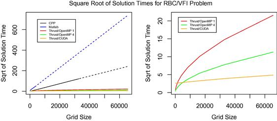
Figure 4 Square root of solution times for serial CPP (black), serial Matlab (blue), single-core Thrust/OpenMP (red), quad-core Thrust/OpenMP (green), and Thrust/CUDA (orange). (For interpretation of the references to color in this figure legend, the reader is referred to the web version of this book.)
When comparing the solution times, it is important to remember that CPUs and GPUs cost different amounts of money. The Tesla C2075 GPU and the quad-core Xeon CPU used in this section cost $2120.79 and $339.03, respectively. This means that one could purchase roughly ![]() quad-core 2.4 GHz Xeon processors for the same amount of money as a single Tesla C2075 GPU. Figure 5 scales all of the computation times by processor cost, resulting in
quad-core 2.4 GHz Xeon processors for the same amount of money as a single Tesla C2075 GPU. Figure 5 scales all of the computation times by processor cost, resulting in ![]() units. For single-core solutions (serial C++, serial Matlab, and Thrust/OpenMP single-core) the times are scaled by 1/4 the price of the Xeon CPU.
units. For single-core solutions (serial C++, serial Matlab, and Thrust/OpenMP single-core) the times are scaled by 1/4 the price of the Xeon CPU.
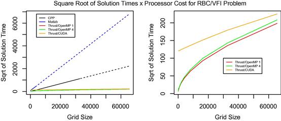
Figure 5 Square root of solution times multiplied by processor cost for serial CPP (black), serial Matlab (blue), single-core Thrust/OpenMP (red), quad-core Thrust/OpenMP (green), and Thrust/CUDA (orange). The single cores solution times (serial C++, serial Matlab, and Thrust/OpenMP single-core) are scaled by 1/4 the cost of the Xeon CPU. (For interpretation of the references to color in this figure legend, the reader is referred to the web version of this book.)
When accounting for cost, the Thrust/OpenMP methods have a slight advantage over the Thrust/CUDA method, with the scaled times approaching each other as ![]() rises. This scaling suggests a slight advantage to purchasing several CPUs rather than one GPU, so long as one uses the Thrust library. However, this assumption does not account for the fact that the Thrust software would not automatically scale across several distinct CPUs—care would have to be taken to rewrite portions of the software to include message passing across devices. Alternatively, purchasing a single CPU with more cores (so that explicit message passing is not required in the Thrust implementation) would drive up the per-core price of the CPU and erode its economic advantage over the GPU. One final consideration is important in this context: several new GPUs are already available which would likely achieve different results for the VFI problem. Two examples are the NVIDIA GeForce GTX Titan and the NVIDIA Kepler K20. The Titan has 2688 cores and costs on the order of $1000 while the K20 has 2496 cores and costs roughly $3200. The low per-core cost of the Titan is due to the fact that it is a consumer-grade GPU which is optimized for single-precision operations (although it is capable of double precision). Relative to the Tesla C2075 with 448 cores, both the Titan and K20 have a much lower per-core cost.
rises. This scaling suggests a slight advantage to purchasing several CPUs rather than one GPU, so long as one uses the Thrust library. However, this assumption does not account for the fact that the Thrust software would not automatically scale across several distinct CPUs—care would have to be taken to rewrite portions of the software to include message passing across devices. Alternatively, purchasing a single CPU with more cores (so that explicit message passing is not required in the Thrust implementation) would drive up the per-core price of the CPU and erode its economic advantage over the GPU. One final consideration is important in this context: several new GPUs are already available which would likely achieve different results for the VFI problem. Two examples are the NVIDIA GeForce GTX Titan and the NVIDIA Kepler K20. The Titan has 2688 cores and costs on the order of $1000 while the K20 has 2496 cores and costs roughly $3200. The low per-core cost of the Titan is due to the fact that it is a consumer-grade GPU which is optimized for single-precision operations (although it is capable of double precision). Relative to the Tesla C2075 with 448 cores, both the Titan and K20 have a much lower per-core cost.
5 Example: A General Equilibrium Asset Pricing Model with Heterogeneous Beliefs
Aldrich (2011) investigates asset exchange within a general equilibrium model with heterogeneous beliefs about the evolution of aggregate uncertainty. This section will outline the model and solution method of that paper and report the computational benefits of GPU parallelism. The economic implications of the model are not treated here. See Aldrich (2011) for a complete discussion.
5.1 Model
The primary objective of the model in Aldrich (2011) is to understand the role of belief heterogeneity in generating trading volume, relative to other forms of agent heterogeneity. The paper demonstrates how small perturbations in agent beliefs can generate empirically plausible levels of trading volume within an economy that is calibrated to broadly replicate macroeconomic consumption dynamics. In order to highlight only the trading effects of belief heterogeneity, the structure of the model is very basic.
We consider a simple endowment economy with ![]() types of agents and
types of agents and ![]() aggregate states of nature each period. Time is discrete and indexed by
aggregate states of nature each period. Time is discrete and indexed by ![]() . The aggregate state at time
. The aggregate state at time ![]() is
is ![]() and we let
and we let ![]() denote the history of aggregate states. Agents’ types are indexed by
denote the history of aggregate states. Agents’ types are indexed by ![]() and
and ![]() denotes the proportion of the population consisting of type
denotes the proportion of the population consisting of type ![]() agents in state
agents in state ![]() . The total population has unit mass, which dictates
. The total population has unit mass, which dictates ![]() , for all
, for all ![]() .
.
There is a single consumption good and a tree paying a dividend of ![]() units of the consumption good in each state
units of the consumption good in each state ![]() , which cannot be transferred between time periods. By default, each agent is entitled to
, which cannot be transferred between time periods. By default, each agent is entitled to ![]() units of consumption in state
units of consumption in state ![]() , resulting in an endowment of
, resulting in an endowment of ![]() for cohort
for cohort ![]() and an aggregate endowment of
and an aggregate endowment of ![]() . Agents have preferences for consumption encapsulated in period utility
. Agents have preferences for consumption encapsulated in period utility ![]() , which is type specific and which satisfies the usual conditions of strict monotonicity, strict concavity, twice continuous differentiability, and
, which is type specific and which satisfies the usual conditions of strict monotonicity, strict concavity, twice continuous differentiability, and ![]() .
.
The aggregate state follows an ![]() -state Markov process: the probability of history
-state Markov process: the probability of history ![]() is
is ![]() , where
, where ![]() is known and hence
is known and hence ![]() . Aside from preference and endowment heterogeneity, encapsulated in
. Aside from preference and endowment heterogeneity, encapsulated in ![]() and
and ![]() , respectively, we allow agent types to have heterogeneous discount factors,
, respectively, we allow agent types to have heterogeneous discount factors, ![]() , and heterogeneous beliefs about transition probabilities,
, and heterogeneous beliefs about transition probabilities, ![]() .
.
Markets are complete and agent types can deviate from their endowments by purchasing state-contingent consumption, ![]() . As discussed below, the results of the paper are unchanged for general asset markets, allowing agents access to assets with varying maturities and payoff structures, so long as markets are complete. The results, however, are easiest to understand within the framework of state-contingent consumption purchases. We denote the time zero price of consumption in state
. As discussed below, the results of the paper are unchanged for general asset markets, allowing agents access to assets with varying maturities and payoff structures, so long as markets are complete. The results, however, are easiest to understand within the framework of state-contingent consumption purchases. We denote the time zero price of consumption in state ![]() as
as ![]() . The resulting optimization problem for an individual agent of type
. The resulting optimization problem for an individual agent of type ![]() is
is
 (17a)
(17a)
 (17b)
(17b)
where ![]() and where
and where ![]() .
.
A competitive equilibrium for this economy is a collection of consumption plans ![]() and prices
and prices ![]() such that
such that
5.1.1 First-Order Conditions
The first-order conditions of System (17) are
![]() (19a)
(19a)
![]() (19b)
(19b)
 (19c)
(19c)
for ![]() , where
, where ![]() is agent
is agent ![]() ’s Lagrange multiplier for constraint (17b). The intertemporal Euler equation is obtained by dividing (19b) by (19a),
’s Lagrange multiplier for constraint (17b). The intertemporal Euler equation is obtained by dividing (19b) by (19a),
![]() (20)
(20)
for all ![]() and
and ![]() . Selecting agent 1 as a “reference” agent, Eq. (20) yields
. Selecting agent 1 as a “reference” agent, Eq. (20) yields
![]() (21)
(21)
Reformulating (21), we arrive at
 (22)
(22)
Substituting Eq. (22) into the aggregate resource constraint (18),
 (23)
(23)
For each ![]() and
and ![]() , given discount rates,
, given discount rates, ![]() , beliefs,
, beliefs, ![]() , period utilities,
, period utilities, ![]() , population proportions,
, population proportions, ![]() , and initial consumption choices,
, and initial consumption choices, ![]() , Eq. (23) represents a single nonlinear equation with a single unknown,
, Eq. (23) represents a single nonlinear equation with a single unknown, ![]() . If
. If ![]() for
for ![]() , the optimal initial consumption values in competitive equilibrium, the values of
, the optimal initial consumption values in competitive equilibrium, the values of ![]() and
and ![]() which solve Eqs. (23) and (22), respectively, will also be the optimal competitive equilibrium values,
which solve Eqs. (23) and (22), respectively, will also be the optimal competitive equilibrium values, ![]() and
and ![]() , for all
, for all ![]() and
and ![]() . In the general formulation, these optimal choices are history dependent.
. In the general formulation, these optimal choices are history dependent.
5.2 Solution
Solving a finite horizon version of this model can become computationally challenging as the time horizon, ![]() , grows large. To solve the model, one would posit values for
, grows large. To solve the model, one would posit values for ![]() and then solve Eqs. (23) and (22) for
and then solve Eqs. (23) and (22) for ![]() at each possible state of the world
at each possible state of the world ![]() prior to
prior to ![]() . The full sequence of optimal consumption values for all agents could then be substituted into the aggregate resource constraint
. The full sequence of optimal consumption values for all agents could then be substituted into the aggregate resource constraint
 (18)
(18)
to determine the quality of the initial guess for ![]() . If the constraint does not hold, an informed update could be made for the initial consumption values and the entire procedure could be repeated to convergence.
. If the constraint does not hold, an informed update could be made for the initial consumption values and the entire procedure could be repeated to convergence.
A serial implementation of the solution would involve an outer loop that forms a candidate solution of optimal consumption values based on a guess for ![]() , and would use the resource constraint in Eq. (18) to iteratively update those values until convergence is achieved. Within the outer loop, a single processing core would then move sequentially through each state
, and would use the resource constraint in Eq. (18) to iteratively update those values until convergence is achieved. Within the outer loop, a single processing core would then move sequentially through each state ![]() , solving the nonlinear Eq. (23) for
, solving the nonlinear Eq. (23) for ![]() and subsequently determining
and subsequently determining ![]() with Eq. (22), conditional on the values
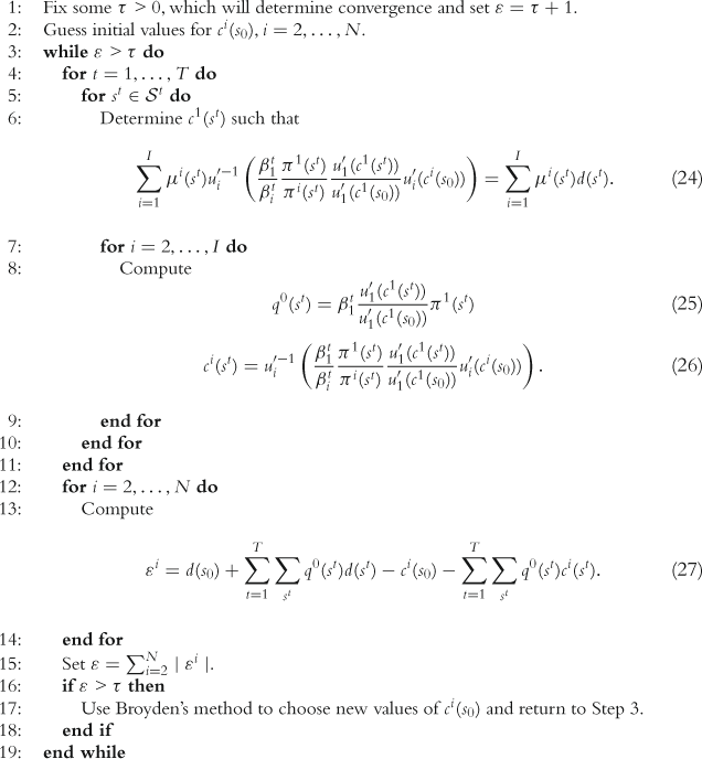
with Eq. (22), conditional on the values ![]() . Algorithm 2 formally outlines these computations: line 3 represents the outer iterative loop, and Eq. (24) represents that nonlinear equation that must be solved at each node in the loops at lines 4 and 5.
. Algorithm 2 formally outlines these computations: line 3 represents the outer iterative loop, and Eq. (24) represents that nonlinear equation that must be solved at each node in the loops at lines 4 and 5.
For a ![]() -period economy, there are a total of
-period economy, there are a total of ![]() states:
states: ![]() at each time period
at each time period ![]() . Clearly, as
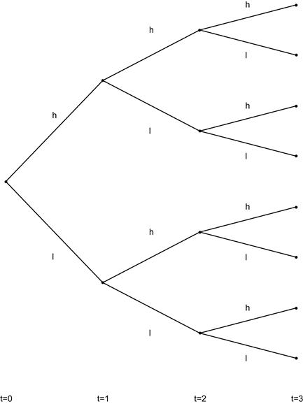
. Clearly, as ![]() grows, the total number of states, and hence systems of nonlinear equations to solve, grows exponentially, which eventually becomes infeasible for a serial processing implementation. Figure 6 depicts an example with
grows, the total number of states, and hence systems of nonlinear equations to solve, grows exponentially, which eventually becomes infeasible for a serial processing implementation. Figure 6 depicts an example with ![]() and
and ![]() . When
. When ![]() this would translate into more than two million nonlinear equations to be solved serially within each of the outer loops of the algorithm.
this would translate into more than two million nonlinear equations to be solved serially within each of the outer loops of the algorithm.
It is important to note that Eqs. (23) and (22) determine a solution for ![]() at each of the
at each of the ![]() states after
states after ![]() , independent of the consumption choices at other dates and states in the economy. This independence between states allows the computation to be divided into distinct pieces, each of which can be performed by a separate processing core. For Algorithm 2, this amounts to outsourcing the work of lines 4–11 to individual cores. In theory, with enough cores, it would be possible to assign the nonlinear equation problem (Eq. (23)) of each state to one core. In practice, with large
, independent of the consumption choices at other dates and states in the economy. This independence between states allows the computation to be divided into distinct pieces, each of which can be performed by a separate processing core. For Algorithm 2, this amounts to outsourcing the work of lines 4–11 to individual cores. In theory, with enough cores, it would be possible to assign the nonlinear equation problem (Eq. (23)) of each state to one core. In practice, with large ![]() or large
or large ![]() , a subset of state-tree nodes would be assigned to each core for computation. In fact, when
, a subset of state-tree nodes would be assigned to each core for computation. In fact, when ![]() and
and ![]() are large, this problem is ideally suited for GPU computing (as shown in the following section).
are large, this problem is ideally suited for GPU computing (as shown in the following section).
5.3 Results
Let us now consider a specialization of the model in Section 5.1 with ![]() and
and ![]() . We will assume that proportions of agent types are fixed through time,
. We will assume that proportions of agent types are fixed through time, ![]() , for
, for ![]() , and that agents have constant relative risk aversion utility,
, and that agents have constant relative risk aversion utility,
 (28)
(28)
Agents receive aggregate consumption, ![]() , as their endowment in state
, as their endowment in state ![]() , where the two aggregate states of nature each period,
, where the two aggregate states of nature each period, ![]() , represent high consumption growth and low consumption growth (
, represent high consumption growth and low consumption growth (![]() ). In particular, we assume that aggregate consumption follows a two-state process
). In particular, we assume that aggregate consumption follows a two-state process
![]() (29)
(29)
where ![]() . The values
. The values ![]() and
and ![]() were estimated by Aldrich (2011) using a hidden Markov model and quarterly NIPA data between 1947 and 2010. The estimates are reported in Table 3 and include estimated transition probabilities between states. In the results reported by Aldrich (2011), the majority of agents maintain beliefs that are consistent with the estimated probabilities in Table 3, while a minority of the population deviates. In particular, that paper considers cases where the minority believes
were estimated by Aldrich (2011) using a hidden Markov model and quarterly NIPA data between 1947 and 2010. The estimates are reported in Table 3 and include estimated transition probabilities between states. In the results reported by Aldrich (2011), the majority of agents maintain beliefs that are consistent with the estimated probabilities in Table 3, while a minority of the population deviates. In particular, that paper considers cases where the minority believes ![]() is one, two, and three standard errors below its maximum likelihood estimate; i.e., they are relatively optimistic. For the present development, where we are concerned with questions of computational efficiency, it is unnecessary to take a stance on the degree of belief divergence and the proportions of agents that subscribe to each view—the timing results are unchanged by these parameters.
is one, two, and three standard errors below its maximum likelihood estimate; i.e., they are relatively optimistic. For the present development, where we are concerned with questions of computational efficiency, it is unnecessary to take a stance on the degree of belief divergence and the proportions of agents that subscribe to each view—the timing results are unchanged by these parameters.
Table 3
Maximum likelihood estimates for the parameters of the aggregate consumption growth process using a hidden Markov model and quarterly consumption data between 1947 and 2010. See Aldrich (2011) for details. Standard errors are obtained from a numerical evaluation of the Hessian.

Table 4 reports timing results for solutions of the model over increasing time horizons ![]() using Thrust/CUDA on the Tesla C2075 and Thrust/OpenMP and all four cores of the Xeon CPU. As with the VFI problem in the previous section, the cost of initializing the CUDA runtime environment (a bit
using Thrust/CUDA on the Tesla C2075 and Thrust/OpenMP and all four cores of the Xeon CPU. As with the VFI problem in the previous section, the cost of initializing the CUDA runtime environment (a bit ![]() s) swamps the overall solution time of the GPU for low values of
s) swamps the overall solution time of the GPU for low values of ![]() —only when
—only when ![]() does the GPU solve the model in less time than the CPU. The efficiency of the multicore CPU solution then erodes very quickly: for
does the GPU solve the model in less time than the CPU. The efficiency of the multicore CPU solution then erodes very quickly: for ![]() it is roughly 10 times slower than the GPU, for
it is roughly 10 times slower than the GPU, for ![]() it is 20 times slower, and for
it is 20 times slower, and for ![]() it is more than 100 times slower. Clearly, as the problem scales (for
it is more than 100 times slower. Clearly, as the problem scales (for ![]() the number of state-tree nodes is roughly 33 million, 130 million, 530 million, and 2 billion, respectively) the relative performance of the GPU increases. These results are remarkable, especially when considering total computational efficiency of each processing unit: the Tesla C2075 is capable of 515 billion floating point operations per second (FLOPS), while the quad-core Xeon is capable of roughly 77 billion FLOPS (both measurements are for double precision arithmetic). These numbers suggest that the GPU should be no more than roughly 6.5 times faster than the CPU. As suggested in Lee et al. (2010b), applying various CPU optimizations might ameliorate the results reported in Table 4. However, such optimizations would be challenging for most economists and the results of this section compare software implementations that are of commensurate difficulty and accessible to the majority of economists. In this sense, these results compare operational efficiency: they compare not only hardware, but also software implementations that require roughly the same level of technical expertise and how they interact with the hardware. As in the previous section, if we scale the solution times by processor cost at
the number of state-tree nodes is roughly 33 million, 130 million, 530 million, and 2 billion, respectively) the relative performance of the GPU increases. These results are remarkable, especially when considering total computational efficiency of each processing unit: the Tesla C2075 is capable of 515 billion floating point operations per second (FLOPS), while the quad-core Xeon is capable of roughly 77 billion FLOPS (both measurements are for double precision arithmetic). These numbers suggest that the GPU should be no more than roughly 6.5 times faster than the CPU. As suggested in Lee et al. (2010b), applying various CPU optimizations might ameliorate the results reported in Table 4. However, such optimizations would be challenging for most economists and the results of this section compare software implementations that are of commensurate difficulty and accessible to the majority of economists. In this sense, these results compare operational efficiency: they compare not only hardware, but also software implementations that require roughly the same level of technical expertise and how they interact with the hardware. As in the previous section, if we scale the solution times by processor cost at ![]() , the GPU is roughly 16 times more efficient (time/dollar) than the quad-core CPU. This is a substantial improvement relative to the VFI problem.
, the GPU is roughly 16 times more efficient (time/dollar) than the quad-core CPU. This is a substantial improvement relative to the VFI problem.
Table 4
Timing results (in seconds) for the heterogeneous beliefs model over increasing horizon ![]() . “Thrust/OpenMP” and “Thrust/CUDA” refer to the Thrust implementation, using the separate backends for OpenMP (on the quad-core Xeon CPU) and CUDA (on the Tesla C2075).
. “Thrust/OpenMP” and “Thrust/CUDA” refer to the Thrust implementation, using the separate backends for OpenMP (on the quad-core Xeon CPU) and CUDA (on the Tesla C2075).

Increasing the complexity of the VFI problem in the previous section translated to greater solution accuracy; in this problem increasing complexity has no bearing on solution accuracy, but increases the time horizon for the model under question. With a quarterly calibration, ![]() (which the CPU can compute quickly) and
(which the CPU can compute quickly) and ![]() (for which the CPU is much slower) correspond to horizons of 5 and 7 years. With multiple GPUs it would be feasible to push the horizon well past a decade, and with a cluster of hundreds of GPUs (such as the Titan supercomputing system at Oak Ridge National Lab: http://www.olcf.ornl.gov/titan/) it would be possible to extend the horizon to several decades. To the extent that important economic decisions are being made at long horizons, being able to compute such models adds real economic value to understanding agents’ decisions. This is true of the model in Aldrich (2011) for which issues of survival play a role in the exchange of assets.
(for which the CPU is much slower) correspond to horizons of 5 and 7 years. With multiple GPUs it would be feasible to push the horizon well past a decade, and with a cluster of hundreds of GPUs (such as the Titan supercomputing system at Oak Ridge National Lab: http://www.olcf.ornl.gov/titan/) it would be possible to extend the horizon to several decades. To the extent that important economic decisions are being made at long horizons, being able to compute such models adds real economic value to understanding agents’ decisions. This is true of the model in Aldrich (2011) for which issues of survival play a role in the exchange of assets.
6 The Road Ahead
Developments in software and hardware will necessarily influence the way we design both GPU algorithms (in particular) and massively parallel algorithms (in general). The current state of the art for GPGPU computing requires algorithmic design that favors identical execution of instructions over heterogeneous data elements, avoiding execution divergence as much as possible. Occupancy (discussed in Section 2.1.3) is another important consideration when parallelizing computations: most current GPUs are only fully utilized when the number of execution threads is on the order of 10,000–30,000. While GPU parallelism in most algorithms can be achieved in a variety of ways, these two issues, divergence and occupancy, direct scientists to parallel schemes that involve a small set of simple instructions executing on a large number of data elements. This is largely a result of the physical hardware constraints of GPUs—the number of transistors dedicated to floating point vs. memory and control-flow operations. In time, as both GPU and other massively parallel hardware changes, the design of algorithms suitable for the hardware will also change. And so, while this paper has provided some examples of algorithmic design for GPU architectures, it is most important for researchers to be aware of and sensitive to the changing characteristics of the hardware they use. The remainder of this section will highlight recent developments in parallel hardware and software and in so doing will cast our gaze to the horizon of massively parallel computing.
6.1 NVIDIA Kepler and CUDA 5
CUDA 5, the most recent toolkit released by NVIDIA on 15 October 2012, leverages the new NVIDIA Kepler architecture to increase productivity in developing GPU software. Among others, the two most notable features of CUDA 5 are dynamic parallelism and GPU callable libraries.
Dynamic parallelism is a mechanism whereby GPU threads can spawn more GPU threads directly, without interacting with a CPU. Previous to CUDA 5, all GPU threads had to be instantiated by a CPU. However, a kernel which is executed by a GPU thread can now make calls to other kernels, creating more threads for the GPU to execute. Best of all, the coordination of such threads is handled automatically by the scheduler on the GPU multiprocessor. This increases the potential for algorithmic complexity in GPU parallel algorithms, as multiple levels of parallelism can be coordinated directly on the GPU. Dynamic parallelism is only available on Kepler-capable NVIDIA GPUs released after 22 March 2012.
GPU callable libraries allow developers to write libraries that can be called within kernels written by other users. Prior to CUDA 5, all GPU source code had to be compiled within a single file. With the new toolkit, however, scientists can enclose GPU software in a static library that can be linked to third-party code. As high-performance libraries are created, this feature will extend the capabilities of individual researchers to write application-specific software, since they will be able to rely on professionally developed libraries rather than writing their own routines for each problem. An example would be simple regression or optimization routines: if an application requires such routines to be called within a GPU kernel, the new CUDA toolkit allows them to be implemented in a third-party library, rather than written personally by an individual developing the particular application. GPU callable libraries only depend on CUDA 5 and not on the Kepler architecture—older NVIDIA GPUs can make use of callable libraries so long as they have the CUDA 5 drivers installed.
GPU callable libraries and dynamic parallelism interact in a way that results in a very important feature: GPU libraries that were previously only callable from a CPU can now be called directly within a kernel. As an example, CUDA BLAS, which leverages GPU parallelism for BLAS operations, can now be called by a GPU thread in order to perform vector or matrix operations. Prior to CUDA 5, vector and matrix operations had to be written by hand if performed within a GPU kernel. This feature, of course, will extend to other GPU libraries which spawn many threads in their implementation.
6.2 Intel Phi
On 12 November 2012, Intel released a new microprocessor known as the Intel Xeon Phi (Intel Corporation (2013b)). To be specific the Phi is a coprocessor which can only be utilized in tandem with a traditional CPU that manages its operations. However, the 50 individual cores on the Phi are x86 processors in their own right, similar to x86 cores in other Intel CPU products. In other words, each Phi core possesses the capabilities of running a full operating system and any legacy software that was written for previous generation x86 CPUs.
The primary objective of the Phi is to introduce many of the advantages of GPU computing within an architecture that doesn’t sacrifice the benefits of traditional CPUs. At 1.05 GHz each, the 50 Phi cores don’t deliver as much raw compute power as a Tesla C2075 GPU, but they allow for far greater functionality since they have many more transistors dedicated to memory use and control flow. This effectively eliminates the issues of thread divergence and allows serial software to be more quickly and easily ported to parallel implementations. It also allows the use of third-party numerical libraries and software without modification.
It is difficult to forecast the nature of future parallel processors, but it is very likely that hybrid processors like the Xeon Phi will become increasingly relevant since they combine the benefits of GPU parallelism with the flexibility that is necessary for a wide variety of computational tasks. Future processors may also synthesize the benefits of the Phi and current GPUs by placing heterogeneous compute cores on a single, integrated chip, overcoming memory transfer issues and simultaneously allowing for greater thread divergence within a massively parallel framework.
6.3 OpenACC
OpenACC (OpenACC (2013)) is an example of a programming standard that allows for high-level development of parallel computation. Developed jointly by Cray, NVIDIA, and PGI, OpenACC allows users to insert compiler directives to accelerate serial C/C++ and Fortran code on parallel hardware (either a CPU or a GPU). In this way, OpenACC is very similar to OpenMP which accelerates serial code on multicore CPUs.
OpenACC is an important example of software that promotes parallelism at a very high level—it requires very little effort to extend serial code to parallel hardware. With some sacrifice of efficiency and flexibility, OpenACC takes GPU computing into the hands of more software designers and offers a glimpse of the future of parallel computing: software which automatically incorporates the benefits of massive parallelism with very little user interaction. Coupled with future advances in hardware, this could dramatically alter the ways in which parallel algorithms are designed.
7 Conclusion
This paper has provided an introduction to current tools for GPU computing in economics and has demonstrated the use of these tools with examples. Sections 4 and 5 demonstrated the benefits of GPU computing for two specific economic problems. For example, a current NVIDIA GPU intended for scientific computing was able to speed the solution of a basic dynamic programming problem by thousands of times relative to a single-threaded C++ or Matlab implementation. Relative to a multithreaded CPU solution making use of the same software library, the GPU gains were more muted: roughly 5 times. GPU parallelism was also striking in the heterogeneous beliefs model of Section 5, where the model solution was 100 times faster on a GPU than a quad-core CPU for long time horizons.
Adoption of GPU computing has been slower in economics than in other scientific fields, with the majority of software development occurring within the subfield of econometrics. Examples include Lee et al. (2010a), Creel and Kristensen (2011), Durham and Geweke (2011), and Durham and Geweke (2012), all of which exploit GPUs within an MCMC or particle filtering framework. These papers demonstrate the great potential of GPUs for econometric estimation, but the examples of this paper also highlight the inherent parallelism within a much broader set of economic problems. The truth is that almost all computationally intensive economic problems can benefit from massive parallelism—the challenge is creatively finding the inherent parallelism, a task which often involves changing the way the problem is traditionally viewed or computed. This paper also provides guidance for determining if that inherent parallelism is well suited for a massively parallel GPU architecture.
The intent of the examples in this paper is to demonstrate how traditional algorithms in economics can be altered to exploit parallel resources. This type of thought process can then be applied to other algorithms. However, since the tools of massive parallelism are ever changing, so will the design of parallel algorithms. The current architecture of GPUs guides the development of parallel software since it places limitations on memory access and control flow, but as these aspects are likely to change with the development of new many-core and heterogeneous processors, the ability to perform parallel computations on many data elements will also change. The overriding objective then is to creatively adapt algorithms for new and changing architectures.
As time progresses, parallel computing tools are becoming more accessible for a larger audience. So why learn the nuts and bolts of GPU computing now? Why not wait a couple of years until it is even more accessible? For many researchers, waiting might be the optimal path. However, a frontier will always exist and pushing the frontier will not only yield returns for computationally challenging problems, but it will also inform economists’ choices about paths for future research. For the economist who is tackling computationally intensive problems and is often waiting long periods of time for a computer to yield solutions, becoming fluent in the tools of this paper and staying at the frontier will pay great dividends.
References
1. Aldrich, E.M., 2011. Trading Volume in General Equilibrium with Complete Markets. Working Paper.
2. Aldrich EM, Fernández-Villaverde J, Gallant AR, Rubio-Ramírez JF. Tapping the supercomputer under your desk: solving dynamic equilibrium models with graphics processors. Journal of Economic Dynamics and Control. 2011;35:386–393.
3. Amdahl GM. Validity of the single processor approach to achieving large scale computing capabilities. In: 1967:483–485. AFIPS Conference Proceedings. 30.
4. Bell N, Hoberock J. Thrust: A Productivity-Oriented Library for CUDA. In: Hwu W-MW, ed. GPU Computing Gems. 2012:359–372. Chap. 26.
5. Charalambous M, Trancoso P, Stamatakis A. Initial Experiences Porting a Bioinformatics Application to a Graphics Processor. In: Berlin: Springer-Verlag; 2005:415–425. Bozanis P, Houstis EN, eds. Lecture Notes in Computer Science. Vol. 3746.
6. Creal, D.D. 2012. Exact Likelihood Inference for Autoregressive Gamma StochasticVolatility Models, Working Paper, pp. 1–35.
7. Creel, M., Kristensen, D. 2011. Indirect Likelihood Inference, Working Paper.
8. Dongarra JJ, van der Steen AJ. High-performance computing systems: status and outlook. Acta Numerica. 2012;21:379–474.
9. Durham, G., Geweke, J., 2011. Massively Parallel Sequential Monte Carlo for Bayesian Inference, Working Paper.
10. Durham, G., Geweke, J., 2012. Adaptive Sequential Posterior Simulators for Massively Parallel Computing Environments,Working Paper, pp. 1–61.
11. Dziubinski, M.P., Grassi, S., 2012. Heterogeneous Computing in Economics: A Simplified Approach, Working Paper.
12. Fulop, A., Li, J., 2012. Efficient Learning via Simulation: A Marginalized Resample-Move Approach, Working Paper, pp. 1–48.
13. Harris MJ, Baxter III WV, Scheuermann T, Lastra A. Simulation of cloud dynamics on graphics hardware. In: Proceedings of Graphics Hardware. Euro-Graphics Association 2003:92–102.
14. Heer B, Maussner A. Dynamic General Equilibrium Modelling. Berlin: Springer; 2005.
15. Intel Corporation, 2011. Intel Xeon Processor E7–8800 / 4800 / 2800 Product Families, Datasheet, 1.
16. Intel Corporation, 2013a. Desktop 3rd Generation Intel Core Processor Family. Desktop Intel Pentium Processor Family, and Desktop Intel Celeron Processor Family, Datasheet 1, pp. 1–112.
17. Intel Corporation, 2013b. The Intel Xeon Phi Product Family, Product Brief.
18. Judd KL. Numerical Methods in Economics. Cambridge, MA: MIT Press; 1998.
19. Kruger J, Westermann R. Linear algebra operators for GPU implementation of numerical algorithms. ACM Transactions on Graphics 2002:908–916.
20. Kydland FE, Prescott EC. Time to build and aggregate fluctuations. Econometrica. 1982;50:1345–1370.
21. Lee A, Yau C, Giles MB, Doucet A, Holmes C. On the utility of graphics cards to perform massively parallel simulation of advanced monte carlo methods. Journal of Computational and Graphical Statistics. 2010a;19:769–789.
22. Lee VW, Kim C, Chhugani J, et al. Debunking the 100X GPU vs CPU Myth: an evaluation of throughput computing on CPU and GPU. In: Proceedings of the 37th, Annual International Symposium on Computer Architecture. 2010b:451–460.
23. Microsoft, 2012. C ++ AMP : Language and Programming Model, Specification.
24. NVIDIA, 2011. NVIDIA Tesla C2075 Companion Processor, Product Brief.
25. NVIDIA, 2012a. Cuda C Programming Guide, Manual.
26. NVIDIA, 2012b. Thrust Quick Start Guide v5.0, Manual.
27. OpenACC, 2013. The OpenACC Application Programming Interface, Version 2.
28. PCI-SIG, 2006. PCI Express 2.0 Base Specification, Specification.
29. Purcell TJ, Buck I, Mark WR, Hanrahan P. Ray tracing on programmable graphics hardware. ACM Transactions on Graphics. 2002;21:703–712.
30. Stokey NL, Lucas Jr RE, Prescott EC. Recursive Methods in Economic Dynamics. Cambridge, MA: Harvard University Press; 1989.
31. Stone JE, Phillips JC, Freddolino PL, Hardy DJ, Trabuco LG, Schulten K. Accelerating molecular modeling applications with graphics processors. Journal of Computational Chemistry. 2007;28:2618–2640.
32. Tauchen G. Finite state markov-chain approximations to univariate and vector autoregressions. Economics Letters. 1986;20:177–181.
1All of the code can be obtained from http://www.parallelecon.com/basic-gpu/.
