8

Derivatives of Periodic Sampling

It is not easy to benefit from application of nonuniform sampling and at the same time not to suffer from the negative effects that usually accompany processing of the signals sampled in this way. To make these anti-aliasing techniques practically applicable, the typical negative effects corrupting this kind of signal processing have somehow to be suppressed. A search for a good approach to this problem has led to the recent development of hybrid sampling methods, discussed in Chapter 10. They are based on the idea of mixing the elements of periodic and randomized sampling in order to gain from exploiting the advantages of both. The derivatives of periodic sampling discussed in this chapter are considered as essential building blocks for composing such hybrid periodic/nonuniform sampling models. Especially useful are periodic sampling point sequences with random skips. As shown in the following chapters, whenever this type of sampling procedure is used, the consequences of the sampling phase shifting have to be understood in order to take them into account. To reveal the essential relationships between the phase shifting of sampling and the sampled signal reconstruction conditions, it is desirable to visualize the involved signal transformation processes. To do this it is suggested that estimation of Fourier coefficients should be considered as a process rather than a calculation of a parameter and that this approach should be used to visualize the dynamics of the involved processes. This proves to be a convenient and productive technique for studies and will be repeatedly used henceforth.

Generation of the pseudo-randomized sampling pulse sequences used for analog-to-digital conversions suitable for alias-free signal processing is yet another essential application of the model for periodic sampling with random skips. The basic considerations that have to be taken into account when designing generators operating on the basis of this model are discussed as well as practical experience obtained in this area.

8.1 Phase-shifted Periodic Sampling

Introducing phase variations into periodic sampling, if performed correctly, leads to suppression of aliasing. To gain from such an approach, it is essential to realize exactly how the conditions for aliasing change when the phase of the sampling process is varied.

8.1.1 Dependence of Aliasing on the Sampling Phase

The popular signal model will be used according to which a signal x(t) is composed of a multitude of sinusoidal components at arbitrary frequencies in a limited frequency band. Suppose that such a signal is sampled periodically. The sampling frequency is denoted as f_s. Then the sampling point process is periodic with the period T = 1/f_s and the signal sample values are taken at sampling instants t_k = kT + ΔT, k = 0, 1, 2,..., where ΔT < T is the phase angle of the sampling point process.

It was discovered a long time ago that the following equality holds for a signal component at frequency f_x and corresponding aliasing frequencies:

where ϕ_m is the phase of the corresponding aliasing frequency. Equality (8.1) is based on the relationships

and

Then

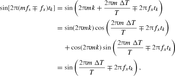
which leads to Equation (8.1). This means that the signal sample values, taken from signal components at frequencies belonging to the row mf_s ∓ f_x, do overlap and that these frequencies are indistinguishable.

Conditions of this overlapping are reflected by the relationships defining the dependence of φ_x on the phase angle of the sampling point process:

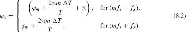
In the case where the sampling phase ΔT = 0 and t_k = kT, k = 0, 1, 2,..., the phase angle ϕ_x does not depend on the phase shift of sampling. Under these conditions the relationship between the phase angle of the signal downconverted to the baseband and the phase of the aliasing frequencies is as follows:

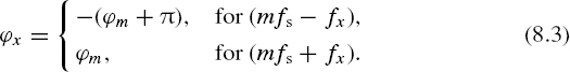
In all other cases, the phase angle ϕ_x also depends on the phase shift of the sampling pulse process. For instance, when the particular aliasing frequency converted down to the baseband [0, 0.5f_s] is f₁ = f_s – f_x, the following equation holds:

Similarly,

and

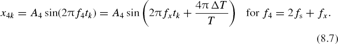
These relationships demonstrate a remarkable fact. They show that conditions for frequency overlapping or aliasing essentially depend not only on the sampling frequency but also on the sampling phase. The fact that the phase angle of the signal, downconverted by aliasing to the baseband, depends on the phase of the sampling point process is illustrated in Figure 8.1. The original signal in this case has just one sinusoidal component at frequency f₁ (Figure 8.1(a)). When it is sampled so that ΔT = 0 (Figure 8.1(b)), the phase angle ϕ_a1 of the alias reconstructed within the baseband [0, 0.5 f_s] is equal to the phase ϕ_x of the original signal (Figure 8.1(d)). If the same signal is sampled at the same sampling frequency but all sampling instants are shifted to a position characterised by ΔϕT = 0.75T (Figure 8.1(c)), the phase angle ϕ_a1 of the reconstructed alias changes in accordance with the relationships (8.2), as shown in Figure 8.1(d), diagram 2.

8.1.2 Reconstruction of Sampled Signals

Consider what happens when reconstruction of a signal sampled at time instants belonging to variable-phase periodic sampling point processes is attempted on the basis of direct and inverse Fourier transforms. The Fourier coefficients are estimated at all frequencies within the frequency band of the signal including the frequencies of a particular row mf_s ∓ f_x. The signal might have a component at the frequency f_x or not, and other components at some of the indicated frequencies mf_s might overlap this specific frequency. In general, the results of Fourier coefficient estimation at this frequency depend on the true signal component, the overlapping aliases and the sampling conditions, specifically the phase of the periodic sampling point process. Attention is drawn to the fact that the phase shift of the sampling point process affects only the overlapping aliases. Variations of this phase do not affect the contribution of the true signal component to the Fourier coefficient estimate at all. There are at least two significant consequences of that:

1. The phase of the periodic sampling point process affects the waveforms reconstructed from the obtained signal sample values.
2. Using variable phase periodic sampling opens up the possibility of avoiding overlapping of the aliasing frequencies.

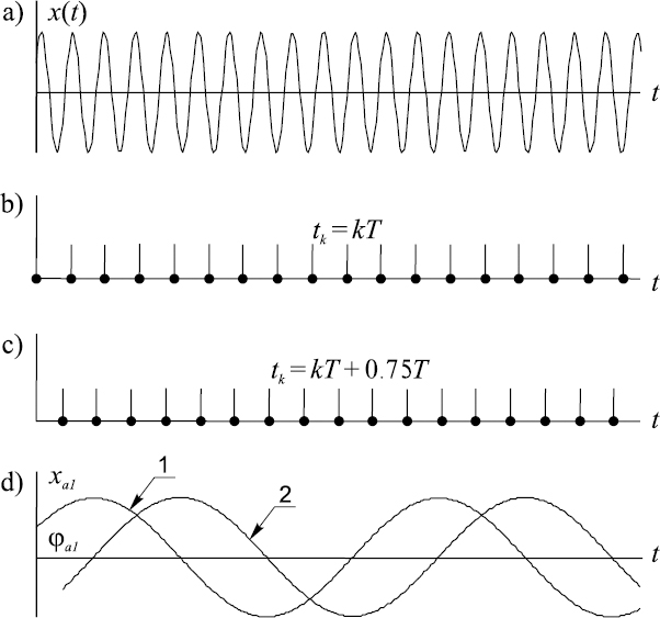
Figure 8.1 Illustration of the fact that the phase angle of the signal, downconverted by aliasing, depends on the phase of the sampling point process

How this possibility might be realized is discussed in Chapter 10. Before studying this essential issue in some detail, variation of the complementary waveforms of signal components at frequencies belonging to the row of the aliasing frequencies mf_s ∓ f_x will briefly be considered. The diagrams shown in Figure 8.2 illustrate this kind of waveform variation, which take place when they are reconstructed from the signal sample values obtained under conditions of variable phase periodic sampling. In this particular case, the analog signal consists of three sinusoids.

Figure 8.2 Waveform variations in the case when they are reconstructed from the sampled signal obtained as a result of variable-phase periodic sampling. The original signal (a) is periodically sampled periodically at different phase shifts: ΔT = 0, 0.25T, 0.5T, 0.75T. Adding the respective reconstructed waveforms (b, c, d, e) provides the waveform (f)

It can be seen from Figure 8.2 that, each of the particular waveforms is actually meaningless. However, using all of them together leads to reconstruction of the original signal. Therefore the information carried by the signal sample values, obtained at variable-phase periodic sampling, makes it possible to avoid aliasing and to reconstruct the original signal not corrupted by frequency overlapping.

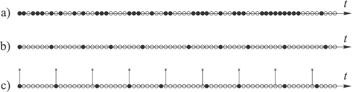
Figure 8.3 Various periodic sampling point processes with random or pseudo-random skips

The result obtained in this particular case is not surprising. Indeed, using four phase-shifted periodic sampling processes in parallel is obviously equivalent to sampling at a frequency four times higher. Actually the purpose of giving this example is just to show that variations of the sampling phase makes it possible to obtain data that might be useful for avoiding aliasing. In the case of processing a stationary signal, such phase-shifted sampling should not necessarily be performed in parallel.

8.2 Periodic Sampling with Random Skips

In many cases of basically periodic sampling, taking of signal sample values at some of the periodically repeating sampling instants is omitted. This kind of sampling might take place either in result of some faults in system functioning or it might be pre-planned and carried out in this way intentionally. We are basically considering the second case. Then the periodic sampling process with random skips is organised and carried out in order to obtain some specific effect. Before discussing particular applications of such sampling, let us consider this general sampling model in some detail.

8.2.1 General Model

The basis of the sampling approach is a periodic point process with randomly or pseudo-randomly excluded sampling points. There are a number of sampling point processes belonging to this category. The difference between them is in the pattern of the skipped sampling points, illustrated in Figure 8.3.

A periodic sampling point process with random skips is shown in Figure 8.3(a). The sampling events take place in this case with some probabilities p_k. Therefore the probability that no sample value will be taken at the sampling time instant t_k is equal to (1 – p_k). As shown in the following chapters, this sampling model is actually a generic one. It represents the basis for decompositions of various sampling point processes and, in addition, it plays an essential role for the hybrid sampling schemes discussed in Chapter 10. It may also be used, for example, to describe a sampling process when some faults occur as a result of electronic system malfunctioning or when faults are due to signal collisions with interfering bursts of noise.

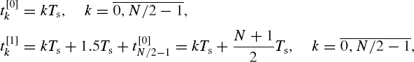
The sampling point processes with pseudo-random skips given in Figures 8.3(b) and (c) define the conditions of sampling performed according to the earlier discussed models of additive and periodic sampling with jitter respectively. However, the sampling schemes in this case are digital and the smallest digit is equal to the period δ of the time grid. Otherwise these schemes are defined as explained in Chapter 6. In the case of additive random sampling illustrated in Figure 8.3(b), signal samples are taken at sampling time instants

where τ_k is a realization of a digital pseudo-random variable.

In a typical pseudo-randomized sampling case, this digital variable is distributed uniformly within the interval [μ ± 0.5Δt], where μ is the mean value of the intervals between the sampling events and the interval Δt < μ so that the distance between two successive sample value taking instants is never shorter than some specified limit. When sampling is performed according to the sampling point pattern displayed in Figure 8.3(c), the sampling instants {t_k} in it are given as

The period T = nδ and the digital variable τ_k is again distributed in an interval shorter than the period.

Of course, these few cases do not exhaust the various sampling schemes based of the model of periodic sampling with random skips. There are more. Nevertheless, all of them have some common features. A high-frequency clock provides their time basis. The frequency 1/δ is usually stabilized. Specific sampling models are then implemented by choosing and setting up a particular scheme, according to which the sampling points are skipped. The pattern of the missing sampling points define most of the characteristics of the resulting specific sampling model. This approach is well suited for organizing various pseudo-randomized sampling modes. The essential advantage of this type of sampling process is the possibility of using for signal processing the information about the exact sample value taking instants and the fixed pattern of the empty slots between the sampling time instants.

8.2.2 Typical Use

Periodic sampling point processes with random skips cover a broad class of various processes often used in the area of randomized digitizing of signals. First of all, the pseudo-randomized clock pulse sequences should be mentioned as the central factor dictating the time instants exactly when the signal sample values are taken according to the time schedule. In addition, they also control other related functions of the respective digitizer. The quality of the sampling pulse sequences, generated according to the preset sampling regime, has to be high as the performance standard of the corresponding system largely depends on it. Execution of the signal processing algorithms is usually based on the assumption that the signal sample values are taken exactly at the predetermined time instants. The reference values generated in the computer are typically tied to these time instants as well. Therefore any discrepancy between the predetermined and realized signal sample value taking acts leads to serious negative consequences. The generation of these pseudo-randomized clock pulse sequences is a responsible function, which needs to be based on a well-developed knowledge basis. A typical example of a developed and successfully exploited electronic system of this kind is given in Section 11.1.

Another area where the periodic sampling point processes with random skips play an essential role is hybrid sampling systems. Although there are various options on how to build such hybrid systems on the basis of combining elements of deterministic and randomized signal processing, they typically use the considered periodic sampling point processes with random skips as essential components, discussed in Chapter 10.

The last but not the least important application area of periodic sampling point processes with random skips is signal processing adapted to sampling nonuniformities. This particular technique has a high application potential and is considered in Chapter 18.

8.3 Compensation Effect

Decomposing periodic sampling point processes with random skips into various frequency periodic phase-shifted components is a technique helping to provide an insight into aliasing processes. In turn this is essential for analysis and synthesis of digital alias-free signal processing algorithms. This technique often provides good results, especially when it is used in combination with the approach to Fourier transforms that presents them as processes rather than just calculations of Fourier coefficients. Then an interesting effect, discussed here as a compensation effect, can be observed. It reveals the essence of alias suppression and shows how this anti-aliasing mechanism works. This effect and examples of its use are described in this section.

8.3.1 Display of Fourier Transforms

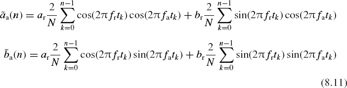
For studies of various side effects of sampling, it is often convenient to use a special approach to Fourier transforms. To realize how and why something happens, application of special functions makes it possible to observe these transforms as processes developing in time. These functions are cumulative sums that are actually the basis for Fourier transforms. They can be given as

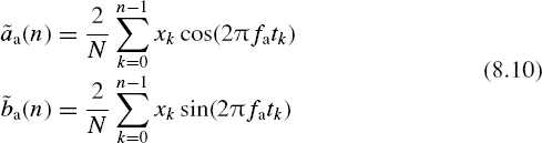
where f_a is the frequency of DFT filtering.

Consider a signal model

where N is the number of the signal samples, f_r = mf_s ∓ f_a, m = 0, 1, 2,... is the signal frequency and f_s is the sampling rate. Substituting into Equations (8.10) yields

To demonstrate the usefulness of this approach, graphical images reflecting DFT filtering of true and aliasing signal components are compared.

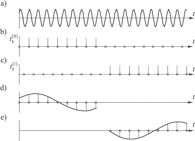
Figure 8.4 Results of sampling a signal according to a two-segment phase-shifted sampling scheme: (a) original signal; (b), (c) phase-shifted sampling point sequences; (d), (e) downconverted signal segments

8.3.2 Observing the Aliasing Processes

Suppose that the defined signal, depicted in Figure 8.4(a), is sampled periodically and after taking the first batch of N/2 sample values the sampling pulse stream is shifted for half of the sampling period so that the following N/2 sample values are taken with this phase shift introduced as shown in Figures 8.4(b) and (c). As the sampling frequency, in the illustrated general case, is lower than the signal frequency, aliasing occurs and the signal is downconverted into the baseband frequencies. The phase angles of the downconverted signal segments change following phase shifting of the sampling process. This effect could be used for reconstruction of the original signal although the sampling frequency is below the Nyquist limit. The reconstructed downconverted signal waveforms are given in Figures 8.4(d) and (e).

Now the cumulative sums introduced in the previous section can be used as a convenient tool for observing the processes related to aliasing. Consider a particular case where

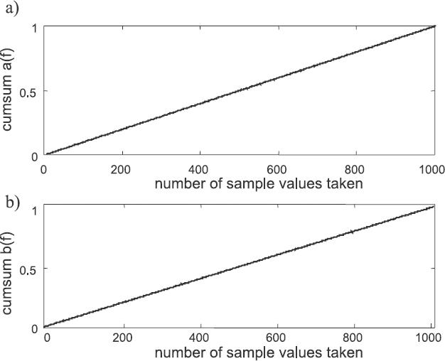
Figure 8.5 Cumulative sums (cumsum) for an existing real signal component

and a_r = 1 and b_r = 1. The signal frequency f_r is set at first below the Nyquist limit and is equal to the filtering frequency f_a. The cumulative sum in this particular case graphically looks like a linearly increasing function for both segments of the sampling process and is shown in Figure 8.5. If the filtering frequency f_a is chosen so that it is equal to an aliasing frequency, then the cumulative sum looks like the broken lines shown in Figure 8.6.

It can be seen from Figure 8.6 that the cumulative sum, obtained for a particular Fourier coefficient in the case where there is a signal component aliasing to the frequency of DFT filtering, is a positively increasing linear function for the first segment of the sampling point process and is equally a negatively increasing function for the second shifted segment of the sampling point process. In other words, the cumulative sum formed at the stage of the first segment is compensated by the cumulative sum accumulated during the time of the second segment of the sampling point process. The end result is close to zero, which it should be in this case when there is no signal at the frequency of analysis and only an aliasing signal component is present.

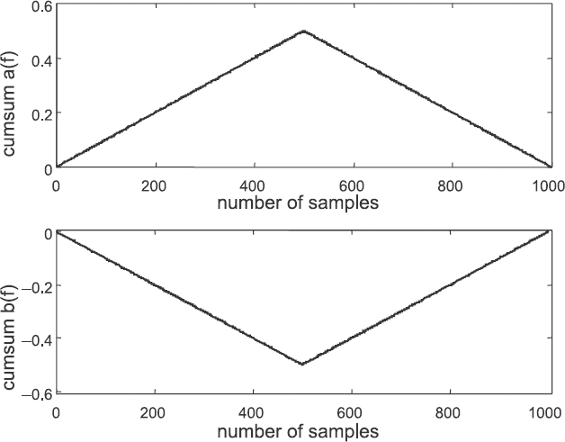
Figure 8.6 Cumulative sums in the case where DFT filtering is performed at one of the aliasing frequencies

Therefore, using the sampling point processes formed by appropriate shifting of segments of the sampling point process produces the compensation effect, taking out the signal aliases as described above. This compensation effect naturally depends on various factors. Nevertheless, it is there and could be exploited with results better than those usually obtained by application of nonuniform sampling. If the involved Fourier transforms could be carried out simply as calculations of the Fourier coefficient estimates, it would be easy not to notice this significant effect, not to observe it and not to take it into account.

The sampling pulse streams, shown in Figures 8.4(b) and (c), are respectively defined as follows:

where T_s = 1/f_s is the period of sampling. Formulae for the respective cumulative sums can be written as follows:

1. For signal frequencies mf_s – f_a and n ≤ N/2, it is found that

   

2. For signal frequencies mf_s – f_a and n > N/2,

   

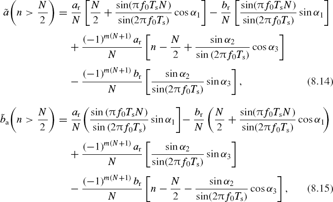
   where

   

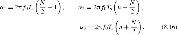
Similar formulae can be derived for signal frequencies mf_s + f_a.

This technique for visualizing the processes related to aliasing is a convenient tool. Application of it for analysis of various signal processing operations often proves to be effective for displaying and presenting them in a comprehensive form. This is demonstrated repeatedly in the following chapters.

8.4 Generation of Randomized Sampling Pulse Trains

Most of the algorithms for digital signal processing are based on the assumption that the time instants of signal sample value taking are known. This condition does not represent a problem for the traditional practice of signal processing. The intervals between the sampling instants are of a constant and known duration and the needed timing data are obtained simply by counting the sampling events. The circumstances are different for processing nonuniformly sampled signals as the intervals between the sampling instants vary by more or less wide margins. Theoretically there are two options: either to measure each sampling interval or to generate the sampling pulses at precisely predetermined instants. As implementing the first option is quite demanding, the second approach to the problem is usually preferable.

Thus the randomized sampling pulse trains, on the one hand, need to be generated according to the requirements of the chosen specific sampling point process and, on the other hand, each pulse has to be generated at the exact predetermined time instant. The generated sampling pulse trains are then used for clocking ADCs and initiating in this way the signal sample value taking.

8.4.1 Basic Approach

The basic principles of generating sampling pulse trains can be easily illustrated using examples of their analog implementations.

Periodic Jittering Pulse Trains

When the distribution of time intervals between successive pulses in the pulse sequence vary within relatively narrow boundaries, pulse trains can be formed in a simple way. A sinusoidal function is generated, a random process ξ(t) is added and the pulses are formed at the time instants when the combined process crosses the zero level.

Additive Random Pulse Trains

It is convenient to use multivibrators to generate this kind of pulse train. Operation of a multivibrator is based on a relatively slow exponential charging and abrupt discharging process of a capacitor. The capacitor is discharged at time instants when the capacitor voltage u_c(t), which increases during the process of charging, reaches some threshold level. In the case of this application, a random process ξ(t) is added to the normally constant threshold level so that this threshold is the sum of a constant voltage u₀(t) and ξ(t). When the power of ξ(t) is negligible, the multivibrator relaxes almost periodically. In cases where the power of ξ(t) is more or less substantial, the discharging instants are more or less influenced by this random process. Multivibrators are appropriate for this application because after the discharges of the capacitor they begin the next charging cycle, disregarding the prehistory without taking the timing of past oscillations into account. This means that intervals between generated sampling pulses are statistically independent as required.

However, this is true only under the assumption that the multivibrators being used are ideal. Under real conditions these intervals may be slightly correlated, but it has been found to be of no real significance. It should be noted that multivibrators become very sensitive to noise during the short time intervals preceding capacitor discharges. This means that the sampling pulse generators of this kind have to be properly screened to prevent their synchronization with outside interference.

Pseudo-random Pulse Trains

The applicability of the analog methods for generating sampling pulse trains is limited. Much more universal are the digital methods. It is important to understand that by using them the problem of forming the sampling pulses is solved in a predetermined way so that their exact positions on the time axis are known beforehand. Such digital sampling pulse trains are actually pseudo-random.

Generation of pseudo-random sampling pulse trains, in principle, is straightforward. They are built on the basis of a periodic clock fulfilling the essential time reference function. To form these pseudo-random pulse trains, pulses are randomly taken from the clock pulse sequence in accordance with the sampling point process to be implemented. A pseudo-random number generator is used to generate the random variables needed for dictating the distances between the generated pulses.

The properties of the pulse trains generated in this way are influenced both by the periodic clock pulse sequence and by the sequence of pseudo-random numbers used. While the latter determines the sampling point density function, characterizing the pulse trains obtained, the former is responsible for aliasing, which may occur if the signals sampled by means of such pulse trains contain components exceeding half the clock frequency.

The most valuable feature of the pseudo-random pulse trains is, of course, that they are fully determined by the clock frequency and by the sequence of pseudo-random numbers used. This means that: (a) such pulse trains can be reproduced at will whenever this is necessary; (b) the nth pulse will always appear at an exactly predetermined instant; (c) descriptions of particular pseudo-random pulse trains can be stored in computer memory and this information can then be used to calculate the time instants when some other required functions or signals should be read out, so that they and the signals are sampled simultaneously.

8.4.2 Practical Experience

While the matter of pseudo-randomized sampling pulse generation at first glance seems to be simple, in reality the situation is different. The performance of digital alias-free signal processing systems directly depends on the quality of the generators producing these sampling pulse sequences. To provide wideband operation in the frequency range up to several GHz and to achieve high precision for signal processing, the sampling pulses often have to be generated with a very short time digit and to be formed very close in time to the respective predetermined instants so that errors do not exceed a few picoseconds. The sampling pulse sequence also has the responsibility of providing a stable and precise time reference. The everpresent jitter needs to be kept within a strictly limited margin as well. Excessive jitter, for instance, leads to spurious frequencies that corrupt signal processing in the frequency domain.

The first decision that has to be taken in the initial stage of designing such a generator is related to the problem of obtaining a precise and stable time reference. One option is to depend on the clock frequency. Implementation of this approach leads to quite good results in the case of relatively low frequency designs. However, the situation is different when the smallest time digit is in the subnanosecond range. For example, when microwave signals are processed digitally at frequencies up to 1 or 2 GHz, the required clock frequency would be twice as much and the necessity to build electronic systems operating at these frequencies substantially complicates the system designs.

In such cases another option based on the use of signal propagation delays as the time reference seems to be more appropriate. This approach could be implemented on the basis of considerably lower frequency electronics and therefore the system designs would then be much simpler. The practical experience obtained confirms this assumption. High-performance sampling pulse generators have been developed and made on this basis. Exploitation of various systems containing this kind of sampling pulse generator has provided good results. However, there is also an intrinsic drawback characterizing this approach. These are problems related to the jitter control. The generation process is then based on switching various time delay elements to generate the sampling pulses with a predetermined proper pattern of nonuniform distances between them. It is relatively difficult to ensure in this case that all generated sampling pulses are placed exactly on the time grid. Hence there are imperfections in the generation process, which are observed as jitter of the sampling pulse generation instants.

It seems that the best approach to the generation of sampling pulse trains is to combine both techniques. This method is illustrated later in Figure 11.3 where a block diagram of a generator implementing this method is shown. Such a combination of these techniques makes it possible to use moderate clock frequencies and the quantity of the used delay elements is reduced to a relatively small number. As a result, the generator shown in Figure 11.3 generates sampling pulses with high precision while the jitter does not exceed a few picoseconds. To form sampling pulses according to a predetermined nonuniform pattern, the pulse forming process is based on controllable division of the clock frequency followed by controllable introduction of time delays. The generator of pseudo-random numbers provides the code for digital control of this process. This is discussed in more detail in Chapter 11.

To continue the illustration of this example, some figures characterizing a particular generator are given. The periodic clock pulses were generated at the rate of 669.3266 MHz. The clock frequency was divided by a random integer ranging from 9 to 16. Then the output pulses were expanded in width (up to approximately 5 ns). An adjustable delay line and a high-speed multiplexer were used to implement a single-bit controllable delay block. As a result, the intervals between the generated sampling pulses at the output of the generator were pseudo-randomly varied from 13.447 to 24.652 ns with the smallest time digit equal to 747 ps. This generator is adapted for joint operation over a wide range of ADCs with the maximum sampling rate over 80 MS/s and a broad analog bandwidth. Although in the particular considered case the mean sampling rate is only 53.546 MS/s, the equivalent sampling rate is much higher, providing for digital alias-free signal processing in the bandwidth up to 669.3 MHz. It should be emphasized that the introduced tight control of the sampling pulse jitter made it possible to achieve a bandwidth free from the spurious frequencies due to sampling imperfections.

Bibliography

Artjuhs, J. and Bilinskis, I. (2006) Method and apparatus for alias suppressed digitizing of high frequency analog signals. EP 1 330 036 B1, European Patent Specification, Bulletin 2006/26, 28.06.2006.

Artyukh, Yu., Bilinskis, I. and Vedin, V. (1999) Hardware core of the family of digital RF signal PC-based analyzers. In Proceedings of the 1999 International Workshop on Sampling Theory and Application, Loen, Norway, 11–14 August 1999, pp. 177–9.

Artyukh, Yu., Bilinskis, I., Boole, E., Rybakov, A. and Vedin, V. (2005) Wideband RF signal digititising for high purity spectral analysis. In Proceedings of the International Workshop on Spectral Methods and Multirate Signal Processing (SMMSP 2005), Riga, Latvia, 20–22 June 2005, pp. 123–8.

Bilinskis, I. and Artjuhs, J. (2006) Method and apparatus for alias suppressed digitizing of high frequency analog signals. United States Patent US 7,046,183 B2, 16 May, 2006.

Bilinskis, I. and Mikelsons, A. (1983) Digital Random Processing of Continuous Signals (in Russian). Riga: Zinatne.

Bilinskis, I. and Mikelsons, A. (1990) Application of randomized or irregular sampling as an anti-aliasing technique. In Signal Processing, V: Theories and Application. Amsterdam: Elsevier Science Publishers, pp. 505–8.