
8
MATHEMATICAL REQUIREMENTS FOR PHYSICAL CHANNELS
8.1 Frequency-Domain Effects in Time-Domain Simulations
8.1.1 Linear and Time Invariance
8.1.2 Time and Frequency–Domain Equivalencies
8.1.3 Frequency Spectrum of a Digital Pulse
8.1.4 System Response
8.1.5 Single–Bit (Pulse) Response
8.2 Requirements for a Physical Channel
8.2.1 Causality
8.2.2 Passivity
8.2.3 Stability
References
Problems
Modern high–speed digital design requires extensive signal integrity simulations to assess the electrical performance of the system prior to fabrication of prototypes. To ensure accurate results from the simulations, careful attention must be given to system component models such as transmission lines, vias, connectors, and packages. For a model to be physically consistent with the laws of nature, certain mathematical constraints must be obeyed to ensure proper balance between signal propagation, energy storage, and losses. For example, the vast majority of engineers designing high–speed digital systems today utilize simplified modeling techniques that employ frequency–invariant values of dielectric permittivity, loss tangent, and inductance for transmission–line models. A review of Chapters 5 and 6 will remind the reader that transmission–line models have frequency–dependent properties that must be modeled correctly if a realistic response is expected. Such assumptions, although valid at low frequencies or for very short electrical structures, induce amplitude and phase errors for digital data rates faster than 1 to 2 Gb/s. In fact, the computer currently being used to write this chapter was designed using traditional modeling techniques, which assume frequency–invariant electrical properties of dielectrics and conductors. Such assumptions, however, cease to produce valid results for higher data rates. As data rates increase, bandwidth demands skyrocket, form factors shrink, and new phenomenan that were insignificant in past designs become significant. When the correct model assumptions are not used, incorrect solution spaces are determined, lab correlation becomes difficult or impossible, and the design time is increased significantly. In this chapter we outline some of the most important techniques used to determine if a physical channel model is adequate for the design at hand. First, the fundamentals of calculating the channel response and methods of implementing frequency–domain phenomena in time–domain simulations are explored. Next, the mathematical requirements for a channel that is consistent with nature are explained, and methodologies for testing these requirements are defined. It is not always necessary for a model to obey these physical rules if the error is small enough; however, it is an important concept for the modern–day digital designer to understand to ensure full comprehension of the modeling assumptions.
8.1 FREQUENCY–DOMAIN EFFECTS IN TIME–DOMAIN SIMULATIONS
Although high–speed digital design is focused largely on the signal integrity of time–domain digital waveforms, many of the phenomena that heavily influence the propagation of signals on interconnects are best described in the frequency domain. Examples covered in previous chapters include skin effect resistance, surface roughness, internal inductance, and frequency–dependent dielectric properties. Consequently, it is important for the digital engineer to understand the relationship between a time–domain waveform and its equivalent frequency–domain representation. In fact, many modern buses have component specifications in terms of frequency–domain parameters because it is the most convenient way to describe the wideband behavior. In this section we outline some of the fundamental principles for linear time–invariant systems that will allow the engineer to translate between the frequency and time domains.
8.1.1 Linear and Time Invariance
A system is linear if the relationship between the input and output of the system satisfies the superposition property. For example, if the input to the system is the
sum of two component signals,
![]()
where C1 and C2 are constants, the output of the system will be
![]()
where yn(t) is the output resulting from the input xn(t) (n = 1 and 2). To generalize, a linear system with input
will have output
for any constants Cn and where the output yn(t) results from the input Xn(t).
Time invariance means that whether an input to the system is applied at t = 0 or t = τ , the output will be identical except for a time delay of τ. For example, if the output due to input x(t) is y(t), the output due to input x(t –τ) is y(t –τ). Simply put, a time delay at the input should produce a corresponding time delay at the output.
8.1.2 Time and Frequency–Domain Equivalencies
Any time–domain waveform in an LTI system has an equivalent spectrum in the frequency domain. This means that any time–domain signal, such as a digital waveform, can also be described fully in terms of its frequency–domain parameters. This concept is important because it allows the frequency–dependent nature of electromagnetic models to be integrated into time–domain waveforms so that the signal integrity of digital bits propagating on a bus can be analyzed. The relationship between a time–domain signal and its frequency–domain equivalent is described with the Fourier transform:
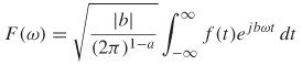
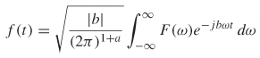
where (8-1a) translates a time–domain signal into a frequency–domain representation and (8-1b) translates the frequency–domain representation into a time–domain waveform. When using the Fourier transform, it is important to ensure that the correct conventions are used. Different technical and scientific fields have different conventions that can confuse the analysis if consistency is not maintained. The conventions are based on the choices for a and b. Some popular conventions are (a = 0, b = –1) for modern physics, (a = 1, b = –1) for systems engineering, (a = –1, b = 1) for classical physics, and (a = 0, b = –2π) for signal processing [Wolfram, 2007]. In this chapter we utilize both the systems engineering and signal processing conventions, depending on the application.
The Fourier transform simply relates a time–domain waveform to a frequency response by superimposing an infinite number of sinusoidal functions to reconstruct the original waveform. For example, if the Fourier expansion of a 50% duty cycle square wave is calculated,
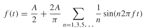
the wave shape can be approximated by superimposing several individual harmonics, as demonstrated in Figure 8-1. As the harmonic n is increased, the reconstructed waveform better approximates the original.
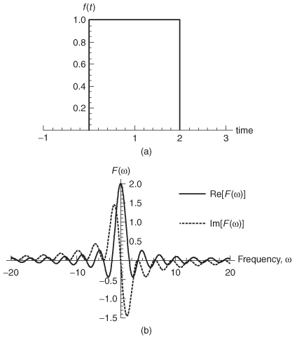
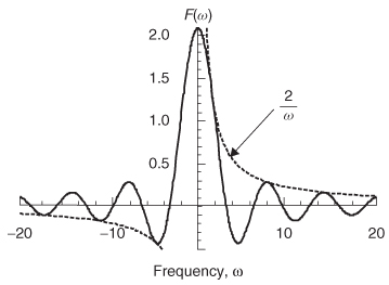
The Fourier transform shown in equation (8-1a) can be used to calculate the real and imaginary parts of the individual sinusoids needed to reconstruct the time–domain waveform, which is known as the spectrum of the waveform. For example, the frequency spectrum of a perfect square pulse, with a width of 2 time units as shown in Figure 8-2a, is calculated using the systems engineering convention (a = 1, b = –1).
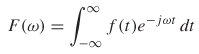
Figure 8-1 Fourier expansion for a 50% duty cycle square wave.
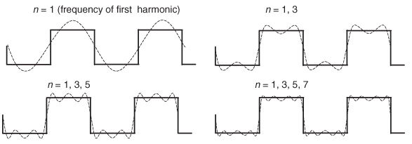
Figure 8-2 (a) Square wave f (t ), which is the most primitive approximation of a digital bit; (b) frequency–domain equivalent spectrum of the square wave.

However, since ![]() the frequency spectrum can be simplified:
the frequency spectrum can be simplified:
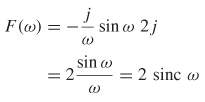
Equation (8-3) is the frequency spectrum of a square–wave pulse and is plotted in Figure 8-2b. This means that the frequency–domain representation of a square wave takes the form of a sinc function, and vice versa. Note that for a perfect step or pulse, an infinite number of harmonics is required to reproduce the waveform.
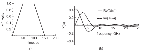
The centering of the square wave around t = 0 in Figure 8-2a simplifies the mathematics by eliminating the imaginary portion of the transform. For a realistic digital pulse with only positive time values, the spectrum becomes complex. For example, the Fourier transform of a square pulse with a width of 2 time units is shown in Figure 8-3 calculated with system engineering conventions (a = 1, b = –1). Note that the spectrum contains both real and imaginary components.
The examples shown in Figures 8-2 and 8-3 demonstrate three very important concepts that link the time–domain waveform to its frequency–dependent equivalent.
1. The spectrum of the time–domain waveform has both positive and negative frequency components.
Figure 8-3 (a) Square wave f (t) with only positive time values; (b) frequency–domain equivalent spectrum of the square wave. Note that the spectrum has both real and imaginary values.
2. The spectrum of a time–domain waveform with only positive time values is complex.
3. Since time–domain signals that are physically observable have no imaginary component, they must be real. Reality in the time domain is guaranteed when the positive frequencies of the Fourier transform are the complex conjugate of the negative frequencies [LePage, 1980]:
The behavior of equation (8-4) can be observed in Figure 8-3b. For example, at the frequency ω = –2 rad/s, the spectrum has a value of
![]()
and at ω = 2 rad/s, the spectrum has a value of
![]()
Since F(–2) = F(2)*, the spectrum is for a real time–domain waveform.
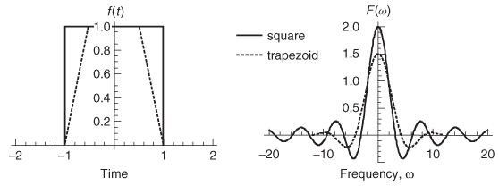
Figure 8-4 Frequency response of a trapezoidal wave compared to an ideal square wave.
8.1.3 Frequency Spectrum of a Digital Pulse
Although a square pulse is a first–order approximation of a digital bit, a better approximation is a trapezoid. Figure 8-4 shows the frequency response of a trapezoidal wave compared to an ideal square wave. Notice the shape of the trapezoid’s frequency response is very similar to that of a square wave, except that the magnitude of the harmonics are smaller, especially at high frequencies. This demonstrates another important concept: The rise and fall times of a digital waveform determine the magnitude of the high–frequency harmonics in the frequency–domain spectrum
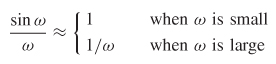
.Figure 8-4 also indicates that the spectrum of a trapezoid can be derived by applying a low–pass filtering function to the spectrum of a square wave. This allows a relationship to be defined between the spectral content of a digital waveform and the rise and fall times. To begin the derivation of this relationship, some unique properties of the square–wave spectrum need to be observed. Equation (8-3) shows that the harmonics of a square wave are a sinc function. Taking the limits of the sinc function allows the frequency spectrum to be generalized:
The quantity 2/m is compared to the spectrum calculated with equation (8-3) in Figure 8-5. Note that the quantity 1/m is equivalent to a slope of 20 dB/decade on a log–log plot:
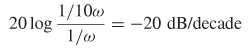
meaning that the spectral content of a square wave will fall off at a rate of –20 dB/decade.
One way to approximate the spectrum of a trapezoidal wave is to apply a low–pass filtering function to the harmonics of a square wave until the desired rise and fall times are realized. The easiest way to apply this filtering is to use a simple low–pass one–pole filtering response, such as an RC network. The step response of a simple one–pole filter is
Figure 8-5 The spectrum of a square wave fits within the envelope of 2/ω at high frequencies.
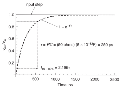
where vinput is the input voltage to the filter, vout the output voltage, and τ the time constant. If the rise times are defined with the 10% and 90% voltage magnitude points, the time constant required to degrade a step to a specific t10–90% can be calculated. The rise time of a unit step after it passes though a one–pole filter with a time constant of τ is calculated as
Note that t10% and t90% are calculated from 0.1 = 1 – e–t10%/τ and 0.9 = 1 – e–t90%/τ. An example is shown in Figure 8-6, where the time constant was calculated assuming an RC network with R = 50 Ω and C = 5 pf.
The 3–dB bandwidth of a one–pole filter is
Solving for τ and substituting into (8–7) produces the well–known relationship between the spectral content of an edge and the rise time:

Figure 8-6 If a unit step is driven into a single–pole network with time constant τ, the resulting 10 to 90% rise time can be calculated.
Equation (8-8) is a good “back of the envelope” calculation that estimates the spectral bandwidth of a digital signal with a rise/fall time of t10–90%.
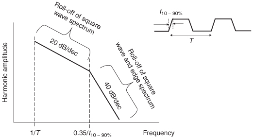
Equations (8–5) and (8–8) can be used to estimate the spectral envelope of a trapezoidal digital signal. The spectrum of a square wave will fall off at –20 dB/decade, as described by (8–5). When the frequency (f3dB) that corresponds to the bandwidth of an edge with rise and fall times of t10–90% is reached, the low–pass filtering function becomes significant, and also falls off at a rate of –20 dB/decade. This allows us to draw the approximate spectral envelope of a digital pulse, as shown in Figure 8-7.
Figure 8-7 Approximation of the spectral envelope of a digital pulse.
8.1.4 System Response
When a system is linear and time invariant, the output and input can be represented with a convolution, where bold face type indicates a matrix:
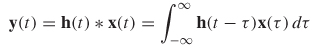
where h(t) is the system impulse response matrix, and each element hij(t) is the response at port i when Dirac’s delta function (an ideal impulse) is applied at port j with all other inputs set to zero. This is an important concept, because if the impulse response of a system is known, the response of the system with any input, X(τ), can be determined.
When the system impulse response is represented in the frequency domain, it is referred to as the transfer function H(ω):
where Y(τ) is the frequency response matrix of the of the system output and X(τ) is the frequency response of the system input. It is usually much more convenient to analyze systems using transfer functions in the frequency domain rather than impulse responses in the time domain. However, due to the equivalency between a time–domain waveform and a frequency–domain spectrum, the inverse Fourier transform of the transfer function is the impulse response:
The relationship of (8–10) is convenient because it is generally much easier to measure the transfer function in the laboratory using a vector network analyzer (VNA) than to measure the impulse response because an ideal impulse is impossible to produce. In fact, in Chapter 9 we describe methods to obtain the impulse response from S–parameters which can be measured in the laboratory using a vector network analyzer. It should be noted that since real laboratory instruments do not provide measured values for negative frequencies, the relationship of equation (8-4) must be used to construct the negative frequency response from the complex conjugate of the positive (measured) frequency response.
Another useful property is that convolution in the time domain is equivalent to multiplication in the frequency domain. Generally, it is much simpler to handle the convolution of an input and an impulse response in the frequency domain by multiplying the spectrums and performing an inverse Fourier transform to convert back to the time domain.
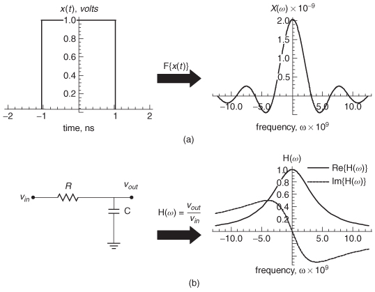
Example 8–1 Determine the wave shape of an ideal, 2–ns–wide square wave propagating through the low–pass RC filter shown in Figure 8-8a. Assume that R = 50 Ω, C = 5 pF, and the amplitude of the square wave is 1 V.
Figure 8-8 (a) Spectrum of a 2–ns–wide square wave for example 8–1; (b) transfer function of an RC filter with R = 50 Ω and C = 5 pF.
SOLUTION
Step 1: Calculate the spectrum of the square wave using equation (8-1a). For this example, system engineering conventions (a = 1, b = –1) were chosen.
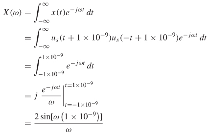
X(ω) is plotted in Figure 8-8a.
Step 2: Calculate the spectrum of the filter. The response of the RC filter can be calculated using basic circuit techniques where the impedance of a capacitor is Zc = 1/jωC:
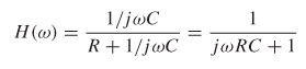
The filter response is plotted in Figure 8-8b. H(ω) represents the transfer function in the frequency domain and the impulse response if converted to the time domain.
Step 3: Calculate the response of the output using equation (8-9b), which is plotted in Figure 8-9a:
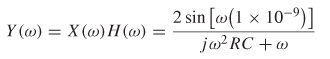
Y(ω) is the frequency–domain equivalent of the pulse after it has passed though the filter. This operation is identical to convolving the filter’s impulse response with the square pulse in the time domain.
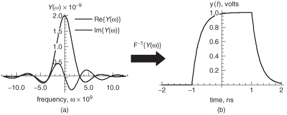
Step 4: Convert Y(a) back to the time domain using equation (8-lb) and system engineering conventions:
![]()
The inverse Fourier transform was evaluated using Mathematica and plotted in Figure 8-9b.
An alternative to the impulse response of a system is the step response. Often, the step response is more conducive to laboratory measurements because time–domain reflection (TDR) instruments are widely available and are capable of injecting rise times as fast as 9–25 ps into a test structure, which can approximate a step function. The unit step function is the integral of the impulse function (Dirac delta function),
Figure 8-9 (a) Spectrum of the driving function for example 8–1 convolved with the filter response; (b) output of the filter when driven with a square wave.
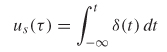
where δ(t) is the impulse function and us(t) is the unit step function.
8.1.5 Single–Bit (Pulse) Response
Perhaps the most useful means to characterize a channel in the time domain is to use the single–bit response, also known as the pulse response. The utility of the pulse response, as opposed to the impulse response, is that it is directly measurable in the laboratory. The pulse response is obtained by driving a system with a waveform that corresponds to a single digital bit of information for the system being designed.
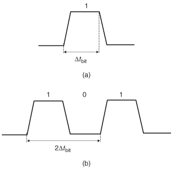
The data rate (DR) is defined as the maximum number of bits per seconds the system will support. This means that the maximum data rate is determined by the width of a single bit:

where Δtbit is the width of a single data bit, as shown in Figure 8-10a. Sometimes, Δtbit is referred to as a unit interval (UI). This means that the maximum fundamental frequency of the digital pulse train, where alternating bits of 1 and 0 are transmitted sequentially, is half the data rate, as shown in Figure 8-10b:
The pulse response is more practical than the impulse response for two reasons. First, the pulse response will give the engineer an intuitive feeling of how the bus will operate because it represents how the system will respond to an actual waveform that will be propagating on the bus. Second, it can be used to calculate the worst–case eye and the worst–case bit pattern using the peak distortion analysis, which is described in Chapter 13.
Analytically, the pulse response is calculated by convolving the input waveform with the system impulse response in the time domain. It is usually more convenient to perform the convolution in the frequency domain,
Figure 8-10 Definitions used to calculate (a) the maximum data rate and (b) the fundamental frequency of a bit stream.
where Y(ω) is the response in the frequency domain, F{Xpulse(t)j is the Fourier transform of the input pulse and H(ω) is the transfer function of the system. The pulse response is then computed by taking the inverse Fourier transform of Y(ω):
Example 8–2 Calculate the 10–Gb/s pulse response of the 0.5–m transmission line calculated in Example 6–4. Assume that the input pulse has rise and fall times of 33 ps and a magnitude of 1 V.
SOLUTION
Step 1: Calculate the real and imaginary parts of the transmission–line transfer function in the frequency domain. This is done with the equation derived in Example 6–4:
![]()
where γ is defined by equation (6–47) and z is the line length,
![]()
and the frequency–dependent values of R, L, C, and G are as calculated in Example 6–4. Next the transfer function is calculated:
![]()
Figure 8-11 (a) Transfer function of the transmission line for example 8–2 (b) impulse response calculated with the inverse Fourier transform of the transfer function.
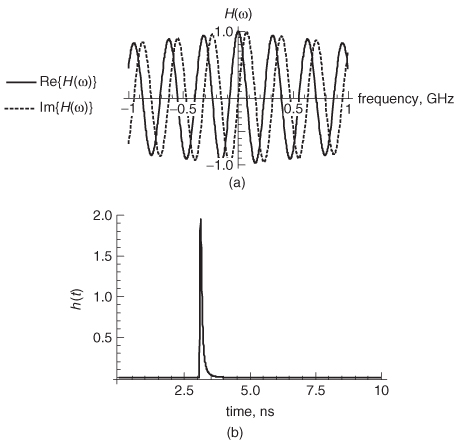
Using the values derived in Example 6–4, the real and imaginary parts of the transfer function are plotted in Figure 8-11a.
Step 2: Calculate the impulse response by taking the inverse Fourier transform of H(ω)) using equation (8-10):
![]()
The impulse response is plotted in Figure 8-11b. Due to the complexity of the integration, for this example the fast Fourier transform (FFT) was used instead of the Fourier integral to evaluate the spectral response of the waveforms. The FFT is a numerical method used to calculate the Fourier transform of an arbitrary waveform. The FFT was equated by sampling the positive and negative frequency response 2000 times in steps of 100 MHz, which gives a time–domain resolution of
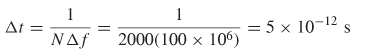
where Δf = 100 x 106 Hz and N = 2000. The FFT is described by Press et al. [2005] and is built into many commercial tools, such as Mathematica, Matlab, Mathcad, and even Microsoft Excel.
Figure 8-12 (a) Waveform driving the transmission line for example 8–2; (b) Fourier transform of the input waveform.
Step 3: Calculate the Fourier transform of the input waveform shown in Figure 8-12a:
![]()
The Fourier transform of the input waveform is plotted for positive frequencies in Figure 8-12b. Note that it takes the familiar form of a sine function. Again, the FFT was used in this example.
Step 4: Calculate the pulse response. First, the spectrum of the pulse response Y(ω) is calculated using equation (8-9b):
![]()
Finally, the pulse response is calculated by taking the inverse Fourier transform of Y(ω):
![]()
The pulse response, which depicts the input waveform after it has propagated from one end of the transmission line to the other, is plotted in Figure 8-13.
Note that the pulse arrives at approximately 3.1 ns. This result can be verified by estimating the total delay from the quasistatic values of the inductance given in Example 6–4 and capacitance using equation (3-107):
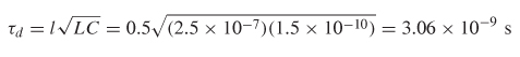
The quasistatic approximation will not be identical to the delay calculated with frequency–dependent parameters, but it should be close. Therefore, the delay of the waveform in Figure 8-13 passes the sanity check.
It is interesting to note how the transmission line distorts the pulse as it propagates down the transmission line. For example, the amplitude of the waveform in Example 8–2 (Figure 8-13) is degraded significantly due to the conductor and dielectric losses. Furthermore, the output pulse is wider than the input pulse because the frequency components of the digital waveform (as calculated with a Fourier transform) will travel at different speeds due to the frequency–dependent dielectric permittivity used to calculate the capacitance. The velocity differences between each harmonic will distort the waveform by spreading it out in time, which is known as dispersion.
Figure 8-13 Pulse response of the transmission line for Example 8–2.

8.2 REQUIREMENTS FOR A PHYSICAL CHANNEL
In this section we introduce specific limitations that channel models of a LTI system must obey to remain physically consistent with nature. Specifically, the conditions of causality, passivity, and stability are described and defined by the appropriate mathematical conditions that must be met to ensure physical behavior. The analysis is restricted to linear and time–invariant electrical networks, which is appropriate for all passive components used in modern bus design, such as transmission lines, vias, packages, connectors, and so on.
8.2.1 Causality
One seemingly obvious requirement of a model that obeys the laws of nature is that an output cannot precede its input. In other words, in the real world we live in, an effect cannot precede its cause. This fundamental principle is called causality. Mathematically, a linear time–invariant system is causal only if for every input all the elements of its impulse response hj vanish for t < 0:
Figure 8-14 Simulated pulse response for a 20–in. transmission line, showing the outputs of a causal and a noncausal model. Note how the noncausal waveform arrives early.
But more generally, if a system has known delay [τ], the system is causal if
An example of a causal and a noncausal pulse response is shown in Figure 8-14, where a pulse response was simulated by driving a 100–ps–wide digital pulse into a causal and a noncausal 20–in. transmission–line model. Note that the noncausal pulse response has a component that arrives early, which is a telltale sign of a nonphysical model. In this example, the noncausal transmission–line model was created using frequency–invariant values of the loss tangent and the dielectric permittivity. The causal model was created using the infinite–pole dielectric model presented in Chapter 6.
Unfortunately, it is not always easy to ascertain whether a model is causal by observing the pulse response. Furthermore, it is not always obvious if it matters. For example, a very short transmission line may be noncausal, but the error could be so small that it would not affect the final result significantly. However, if numerous noncausal models are cascaded together to simulate a bus, the causality errors could accumulate and significant waveform miscalculations could be realized. Fortunately, it is not very difficult to create a causal model by ensuring that the dielectric and conductor properties outlined in Chapters 5 and 6 are followed.
The discussion above prompts an inevitable question: What are the mathematical conditions that specify whether or not a system is causal? To begin, the frequency response of the model is observed. If the Fourier transform of the Don’t get the pulse response confused with the impulse response [h(t)]. Since pulse responses are more representative of a realistic digital driver, they are often used to analyze interconnects.
impulse response h(t) is equated, the frequency–domain equivalent H(a) can be used to test for the conditions of causality:
![]()
The properties of the Fourier transform can be used to make some initial conclusions about the causality of a system.
1. If h(t) is real, H(–a) = H(a)*, where * indicates the complex conjugate [LePage, 1980]. Since time–domain waveforms are always real, this is a necessary requirement.
2. If h(t) is real and odd, H(a) is imaginary and odd [O’Neil, 1991].
3. If h(t) is real and even, H(a) is real and even [O’Neil, 1991].
As a reminder, odd and even functions obey the following rules: Let f (t) be a real–valued function of a real variable. Then f is even if
f(t) = f(–t)
and odd if
–f(t) = f(–t)
This means that if h(t) is even or odd, there will exist a nonzero value for t < 0, which violates the definition of causality as expressed in equation (8-14a).
Another useful property is that the vector space of all real–valued functions is the direct sum of the subspaces of even and odd functions. In other words, every function can be written uniquely as the sum of an even function and an odd function:
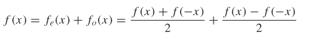
Therefore, a causal function [where h(t) = 0 for t < 0] must be the sum of an even function he(t) and an odd function ho(t).
Consequently, for h(t) to be causal, h(t) must be composed of both odd and even functions. Therefore, based on Fourier transform properties 2 and 3 above, H(a) must have both a real and an imaginary part. For an impulse response h(t) to be real and causal, H(a) must be complex and satisfy the complex–conjugate rule shown in condition 1 above.
However, just because H(ω) is complex obviously does not guarantee causality. Equation (8-15) shows how the negative time components of the odd and even functions must cancel each other out to ensure a causal response. Since the odd and even values of h(t) are generated from imaginary and real parts of H(ω), respectively, causality requires a specific relationship between Re[H(ω)] and Im[H(ω)].
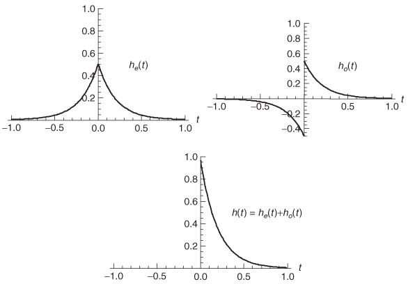
To demonstrate the relationship between Re[H(ω)] and Im[H(ω)], consider a simple causal system with the impulse response h(t) = us(t)e–pt, where us(t) is a unit step function with a value of 0 for t > 0 and a value of 1 for t > 0 and p < 0. Following equation (8-15), the odd and even functions of h(t) can be written:
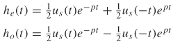
The functions he(t), ho(t), and h(t) and are plotted in Figure 8-15. Note that when ho(t) = he(t) for t > 0 and ho(t) = –he(t) for t > 0, the output h(t) is zero for t < 0 and therefore causal. This allows the odd function to be written in terms of the even component:
Figure 8-15 The odd and even functions are summed to produce the final causal impulse response h(t).
where sgn(t) = 1 and sgn(–t) = –1. Now the causal impulse response can be written in terms of only the even component:
In the frequency domain, H (ω) can also be written in terms of the even function using the property that multiplication in the time domain is the same as convolution in the frequency domain and F{sgn(t)} = –j(1/πω) using the signal processing convention (a = 0, b = –2π) of equation (8-1a):
Equation (8-18) can be simplified by using the definition of a Hilbert transform, which is the convolution of a function g(a) and 1/πω:
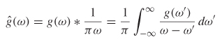
Therefore, equation (8-18) can be written in terms of the Hilbert transform of the even function:

where ![]() e(a) denotes the Hilbert transform of He(ω).
e(a) denotes the Hilbert transform of He(ω).
Equation (8-20) demonstrates two very important properties of a system that will produce a real, linear, and causal response in the time domain.
1. The imaginary part of the frequency response is determined by the Hilbert transform of the real part. Knowledge of the real part is sufficient to define the entire function.
2. Causality can be tested by performing the Hilbert transform of the real part and ensuring that it is identical to the imaginary part.
Note that the real part of a causal signal can be derived from its imaginary part also. It is interesting to note that the Kramers–Kronig relations mentioned in Chapter 6 are another form of the Hilbert transforms that relate the real and imaginary parts of the complex dielectric permittivity to each other.
(6-34a)
(6-34b)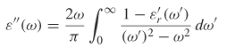
As described in Section 6.4.1, there is a specific relationship between e′(o) and e″(o) that must be enforced to ensure realistic behavior. If the dielectric models do not satisfy the Kramers–Kronig relations, the system will be noncausal.
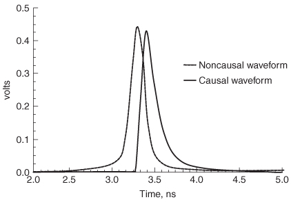
Example 8–3 Use the Hilbert transform to prove that the waveform shown in Figure 8-16a is noncausal and the waveform depicted in Figure 8-16b is casual.
SOLUTION
Step 1a: Calculate the Fourier transform of the noncausal waveform (Figure 8-16a) using the signal processing convention (a = 0, b = –2π) of equation (8-1a):
![]()
Step 2a: Calculate the Hilbert transform of the real part of F (ω) and compare it to the imaginary part:
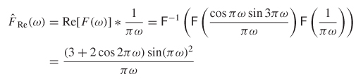
Since Im[F(ω)] = – FRe(ω), the waveform depicted in Figure 8-16a is noncausal. Of course, simple observation of the waveform for this example is proof of noncausality since it exhibits nonzero values for t < 0.
Figure 8-16 (a) Noncausal and (b) causal waveforms for Example 8–3.
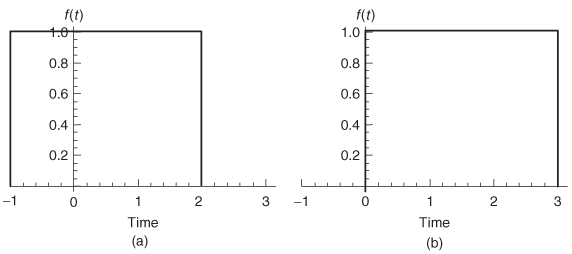
Step 1b: Calculate the Fourier transform of the causal waveform (Figure 8-16b):
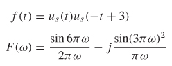
Step 2b: Calculate the Hilbert transform of the real part of F(a) and compare it to the imaginary part:
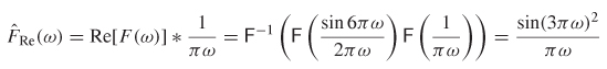
Since Im[F(ω)] = – F7Re(a), the waveform depicted in Figure 8-16b is causal. Of course, simple observation of the waveform for this example is proof of causality since it exhibits only zero values for t < 0.
During bus design, commercial simulation tools are used to implement the models and generate a system response used to evaluate the signal integrity. Each simulator will have its own assumptions, approximations, and numerical methods that may affect causality. The methods detailed above should be used to verify that causal models are being generated. A practical method of judging causality is to observe the rising edge of a pulse response to see if a portion of the signal is arriving early, as demonstrated in Figure 8-14. If a portion of the pulse is arriving early, the system is noncausal. Although this method is less reliable than the rigorous methods defined above, it will provide a general idea if the model is causal.
Example 8–4 Use the Hilbert transform to determine the causality of a transmission line with a length of z = 2.0 in. (~0.05 m) that is terminated perfectly with a relative dielectric permittivity of εr = 4.0, μr = 1, and a decay factor of α = 0.00000001 |f |.
SOLUTION
Step 1: Calculate the transfer function of the transmission line. Since the transmission line is perfectly terminated, no reflections will be generated. Therefore, the loss–free voltage wave will behave as described by equation (3-29). However, since this is not a loss–free network, the voltage equation must be multiplied by the decay factor e–αz:
![]()
Therefore, using equation (2-31) to simplify, the voltage is
![]()
From equations (2–45), (2–46), and (2–52), the propagation constant is calculated:
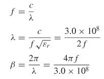
and the transfer function is calculated:
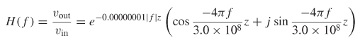
The real and imaginary parts of H(f) are plotted in Figure 8-17a.
Figure 8-17 (a) Transfer function of the transmission line for Example 8–4; (b) Hilbert transform of the real part of H (f) compared to the imaginary part of H (f), showing that the model is noncausal.
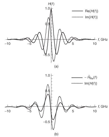
Step 2: Calculate the Hilbert transform of the real part of H(f) compare it to the imaginary part of H(f).
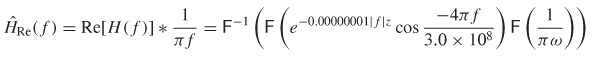
The quantity –![]() Re (f) and the imaginary part of H(f) are plotted in Figure 8-17b. Since Im[H(f)] = –
Re (f) and the imaginary part of H(f) are plotted in Figure 8-17b. Since Im[H(f)] = –![]() Re(ω), the transmission–line model is noncausal. The noncausal nature of this model can also be observed by looking at the impulse response, which is calculated by taking the inverse Fourier transform of H (f):
Re(ω), the transmission–line model is noncausal. The noncausal nature of this model can also be observed by looking at the impulse response, which is calculated by taking the inverse Fourier transform of H (f):
![]()
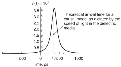
and is plotted in Figure 8-18. Note how the impulse response rises prematurely. The theoretical delay of this transmission line can be calculated from the length, the speed of light, and the relative dielectric permittivity.

Since the transmission line is 2 in. long, the pulse should arrive at τd = (169.333 x 10⁻¹²)(2.0) = 339 ps. It is obvious that the waveform has components arriving much earlier than 339 ps, indicating that the model is noncausal and is not obeying the limits placed on the speed of light.
Figure 8-18 Noncausal impulse response of the transmission line of Example 8–4.
The causality problems associated with the transmission line in Example 8–4 are caused by the assumption of frequency–independent dielectric properties. In Chapter 6 we described numerous dielectric models that show how the dielectric permittivity is frequency dependent. Furthermore, the relationship between the dielectric permittivity and the dielectric losses must be maintained; otherwise, energy will propagate when it should be attenuated, inducting noncausal errors. The dielectric models described in Chapter 6 will produce causal responses when used to simulate transmission lines. Unfortunately, many commercially available simulators do not account properly for the frequency dependence of the dielectric. Consequently, the engineer should be very wary of prepackaged transmission–line models to ensure that physical behavior is being observed in the simulations.
In reality, performing the Hilbert transform analytically is difficult, and numerical methods have to be used. Also, with bandlimited frequency responses, the Hilbert transform may not be a good check for causality, due to aberrations in the time–domain waveform, which is discussed briefly in Example 9–8.
8.2.2 Passivity
A physical system is passive when it is unable to generate energy from within. For example, an n–port network is said to be passive if
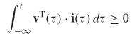
where vT (τ) is the transpose of a matrix containing the port voltages and i(τ) is a matrix containing the currents. The integral (8–21) represents the cumulative net power absorbed by the system up to time t. In a passive system, this quantity must be positive for all t.
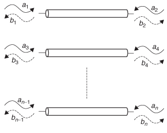
A more useful approach for digital designers would be to test the passivity in terms of the incident (ai) and exiting (bi) power waves at each port, as defined in Section 9.3 and shown in Figure 8-19.
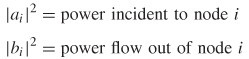
This approach is particularly useful because in Section 9.3.1 it will be developed into a practical passivity test using S–parameters.
Since power must be conserved, the power absorbed by the network (Pa) is equal to the power driven into the network minus the power flowing out:
where Pa ≥ 0 for a passive network. If Pa < 0, the network is generating power and the system would be considered nonpassive.
When working in the frequency domain, the power waves ai and bi will be complex. Since power is real, equation (8-22) must be implemented using the
Figure 8-19 Power waves for an n–port system.
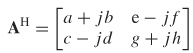
Hermitian transpose, where the complex conjugate of each term is taken, and then the matrix is transposed. For example, consider matrix A:
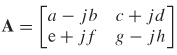
where the Hermitian transpose is AH:
This allows equation (8-22) to be written in terms of the power wave matrices that will produce a real value for the power absorbed by the network. A system is passive if
where a is a matrix that contains all the power waves incident to each port and b contains the power waves coming out of each port. The product of a matrix with complex values and its Hermitian transpose produces a real value. Therefore, equation (8-23) simply ensures that the total power absorbed in a network is greater than or equal to zero.
In the frequency domain, (8–23) is evaluated at each frequency point. In the time domain, the passivity requirement is essentially the same, except that the function must be integrated:
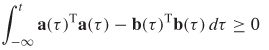
where the transpose is used instead of the Hermitian transpose because timedomain signals are always real. Equations (8–21), (8–23), and (8–24) represent the cumulative energy absorbed by the system. A system is passive only if the following requirements are met:
1. The system absorbs more energy than it generates.
2. Generation of energy happens after the absorption. A noncausal system that generates energy before it absorbs it would be considered to be nonpassive.
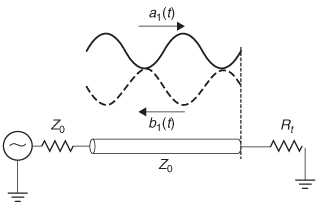
Example 8–5 Determine if the transmission–line system depicted in Figure 8-20 is passive.
SOLUTION
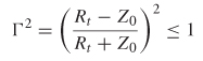
Step 1: Calculate the power waves. The incident wave is a1( t). The reflected wave b1(t) is determined from the reflection coefficient between the termination resistor Rt and the transmission–line impedance Z0. Using equation (3-102), the reflection coefficient is calculated:
![]()
Therefore, the reflected wave is calculated as
![]()
which arrives at the input at t = 2τd, which is twice the electrical length of the transmission line as defined in equation (3-107).
Figure 8-20 Power waves for Example 8–5.
Step 2: Test for passivity. Since this example is in the time domain, equation (8-24) is used:
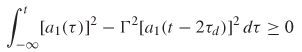
It is easy to see that the integral above will be positive as long as the square of the reflection coefficient is less than or equal to 1 (![]() 2 ≤ 1). This puts a limitation on the termination resistance Rt.
2 ≤ 1). This puts a limitation on the termination resistance Rt.
The only condition where ![]() 2 > 1 is when Rt is negative. Therefore, the system is passive as long as Rt ≥ 0.
2 > 1 is when Rt is negative. Therefore, the system is passive as long as Rt ≥ 0.
8.2.3 Stability
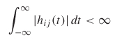
A model of a passive component such as a transmission line, via, connector, or package must remain stable in order to mimic real–world behavior successfully. For the purposes of this book, stability will be defined so that the output of a system y(t) is stable for all bounded inputs x(t). Using this definition, the stability of a linear time–invariant system is guaranteed only if all the elements in the impulse response matrix [h(t)] satisfy [Triverio et al., 2007]
Example 8–6 Determine the conditions of stability of a mass–spring system similar to that used to derive the frequency dependence of the dielectric permittivity in Section 6.3.2. Assume that the system is subjected to a sharp impulse at time t = τ . The spring equation is given:
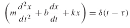
SOLUTION
Step 1: Solve the differential equation and compute the impulse response. For simplicity sake, assume initially that m = 1, b = 3, and k = 2. Since the inverse Laplace transform of the transfer function is the impulse response, it is easiest to solve this problem by converting to the Laplace domain:
![]()
where the Laplace transform of the input is L[γ(t –τ)] = e–τs. From equation (8-9b), Y(s) is solved, where X(s) = e–τs:
and H(s) is the transfer function, which is determined from the roots of the characteristic equation:
The inverse Laplace transform of H (s) yields the impulse response in the time domain:
![]()
Step 2: Check the stability criteria. The system is stable of the integral of equation (8-25) converges:
At t = ∞, the integral is zero, so the integral converges and the system is stable. The impulse response to the system can be plotted by multiplying h(t) by the unit step function us(t –τ), which occurs at time t = τ:
![]()
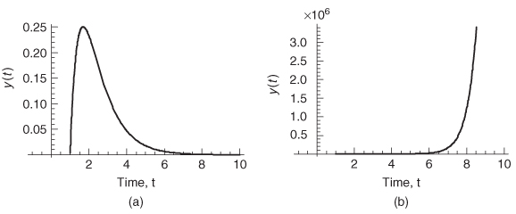
Assuming that τ = 1, Figure 8-21a shows the response of this system.
Now consider the case where the damping coefficient b is negative, which means that the system must generate energy, which is clearly not possible for a damped mass–spring system. Assume that that m = 1, b = –3, and k = 2, which yields
![]()
Figure 8-21 Impulse response of a mass–spring system (Example 8–6) with (a) a positive damping coefficient that is stable and (b) a negative damping coefficient that is divergent and therefore unstable.
The roots of the characteristic equation give the following transfer function:

which yields
![]()
When plugged into equation (8-25) to test for stability, it clearly does not converge and therefore is unstable when the damping coefficient b is negative. Assuming that τ = 1, Figure 8-21b shows the response of this system.
During bus design, simulators such as HSPICE are generally used to implement the models and generate a system response used to evaluate the signal integrity. Each simulator will have its own assumptions, approximations, and numerical methods that will affect stability. Consequently, a practical method of testing stability is to generate a pulse response by driving the model with an ideal trapezoid with edge rates approximating those of realistic drivers. The transient simulation should be evaluated for a time period much longer than the time constant of the model. For example, if the propagation delay of a 10–in. bus is 1.5 ns, the reflections should have diminished to zero within two or three round trips (3 to 4.5 ns). However, the simulation should be evaluated for at least 10 round trips (30 to 45 ns) to ensure that the system remains stable.
REFERENCES
LePage, Wilbur P., 1980, Complex Variables and the Laplace Transform, Dover Publications, New York.
O’Neil, Peter V., 1991, Advanced Engineering Mathematics, Wadsworth, Belmont, CA.
Press, William H., Saul A. Teukolsy, William T. Vetterling, and Brian P. Flannery, 2005, Numerical Recipes in C++, 2nd ed., Cambridge University Press, New York.
Triverio, Piero, Stefano Grivet–Talocia, Michel Nakhla, Flavio Canavero, and Ramachandra Achar, 2007, Stability, causality and passivity in electrical interconnect models, IEEE Transactions on Advanced Packaging, vol. 30, no. 4, Nov.
Wolfram, Stephen, 2007, Mathematica™ 6.0 On–Line Manual, Mathematica, Champaign, IL.
PROBLEMS
8-1 Derive an equation and draw a plot that approximates the spectral bandwidth for a digital waveform with 20 to 80% rise times.
8–2 If a perfect step was driven onto a 50–Ω transmission line terminated in a 5–pF capacitor, what would the rise time be?
8-3 How many harmonics are necessary to adequately represent the bandwidth of a 10–Gb/s pulse with 25–ps rise and fall times?
8–4 For a causal waveform, derive the real part of the spectrum from the imaginary part.
8–5 For an arbitrary time–domain waveform, devise a test to determine if the waveform is causal. Implement your causality tester in a program such as Mathematica or Matlab. Prove that your causality tester works using ideal square–wave inputs.
8–6 Create a causal and a noncausal microstrip model for a 50–Ω transmission line built on FR4 (er at 1 GHz = 3.9, tan S = 0.019) with a 5–mil–wide smooth copper signal conductor (no surface roughness). Evaluate the causality of your models with the tester developed in Problem 8–5.
8–7 Would the noncausal model of Problem 8–6 cause significant error for a 10–Gb/s bus design with transmission–line lengths of 15 in.? If so, how did you determine the impact of the causality error?
8–8 For the transmission line described in Problem 8–6, how does surface roughness influence the causality of the system?
8–9 For the transmission line described in Problem 8–6, what has more of an effect on the causality of the model, the conductor characteristics or the dielectric characteristics? Demonstrate how each affects the causality.
8–10 Is it possible for a real, causal time–domain waveform to have only real frequency components? Show proof of your answer.
8–11 For a loss free system, do the capacitance and inductance matrices need to be frequency dependent to guarantee causality? Show proof of your answer.