CHAPTER TWO

Electromagnetic Scattering

2.1 MAXWELL'S EQUATIONS

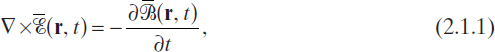
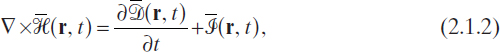
The electromagnetic field is governed by a set of experimental laws known as Maxwell's equations (Stratton 1941, Jones 1964, Felsen and Marcuvitz 1973, Van Bladel 2007, Chew 1990), which relate the field vectors to their sources. Maxwell's equations can be expressed in the following local forms:

Here r denotes the position vector [in meters (m)] and t the time [in seconds (s)]. and are the vector fields describing the electromagnetic field and are called the electric field [in volts per meter (V/m)], the magnetic flux density [in webers per meter (Wb/m²)], the magnetic field [in amperes per meter (A/m)], and the electric flux density [in coulombs per square meter (C/m²)], respectively. The sources are specified by the volume electric charge density ρ [in coulombs per cubic meter (C/m³)] and by the electric current density [in amperes per square meter (A/m²)].

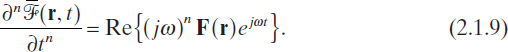
When the time dependence is of cosinusoidal form (time-harmonic fields), a complex representation for field vectors and sources can be used. More precisely, if

is any of the vectors given above, and

where ω is the angular pulsation [in radians per second (rad/s)] [which is related to the frequency f, in hertz (Hz), by ω = 2πf], then it is possible to introduce the complex vector field given by

where , p = x, y, z, such that

In this way the vector field (r, t) is completely described by F(r) when ω is known. Using these relations, it follows that

Taking into account equations (2.1.8) and (2.1.9), the following local form of Maxwell's equations for time-harmonic fields can then be deduced, where E, B, D, H, ρ, and J denote the complex quantities describing the vector fields and their sources:

From the differential form of Maxwell's equations we can derive the corresponding integral forms, which describe the relations among sources and field vectors inside a given region of space (Balanis 1989). By integrating equations (2.1.10) and (2.1.11) over an oriented open regular surface S and applying the Stokes theorem, one obtains

where is the normal to S and C is its contour line, oriented according to S. Analogously, by integrating equations (2.1.12) and (2.1.13) over a bounded volume V and applying the divergence theorem, one obtains

where S denotes the closed surface with normal enclosing the volume V.

Equations (2.1.14)–(2.1.17) are referred to as the global (integral) form of Maxwell's equations.

2.2 INTERFACE CONDITIONS

The field vectors are continuous functions of spatial coordinates except possibly at the boundaries between different media (or where the sources are present). The behavior of the electromagnetic field at the interface between two different media is governed by the interface conditions, which can be simply derived by using the Maxwell's equations in their integral form (Stratton 1941). For time-harmonic fields, the boundary conditions read as

where the subscripts 1 and 2 denote the fields in media 1 and 2, respectively. Moreover, J_s(r) and ρ_s(r) are the surface electric current density (A/m) and the surface charge density (C/m²), possibly lying on the interface between the two media. Finally, indicates the normal to the boundary surface directed toward medium 2.

An interesting particular case occurs when medium 1 is a perfect electric conductor (PEC). In this situation, the time-harmonic field vanishes inside region 1 (Balanis 1989). Consequently, E₁(r) = 0 and H₁(r) = 0 and the interface conditions with a PEC region are given by

On the other hand, it is important to note that surface sources can be induced only on a PEC.

2.3 CONSTITUTIVE EQUATIONS

Maxwell's equations state relationships between the vector fields D, E, B, and H, and their sources J and ρ, which hold true in every electromagnetic phenomenon. However, they are not sufficient for determining the vector fields univocally. In fact, as can be easily proved (Jones 1964), Maxwell's equations [(2.1.10)–(2.1.13), correspond to six independent scalar equations, whereas the four unknown vector fields can be represented by 12 unknown scalar functions. This fact suggests that some further information on the vector fields is needed. Namely, Maxwell's equations [(2.1.10)–(2.1.13)] contain no information on the media in which the electromagnetic phenomena occur. This kind of information is provided by the constitutive equations, which interrelate the vector fields D, E, B, and H, and are specific for the medium where the propagation takes place (Jones 1964). In a very general framework, constitutive equations can be written as

where F and G are operators that associate with every pair of vector fields E and H the vector fields D and B, respectively. As will be shown below, the properties of these operators are used in classification of the constitutive equations.

It is worth noting that vector relations (2.3.1) and (2.3.2) provide six scalar conditions that are to be coupled with Maxwell's equations [(2.1.10)–(2.1.13)]. Equations (2.3.1), (2.3.2), and (2.1.10)–(2.1.13) constitute a system of 12 scalar equations with 12 unknown scalar functions.

An important category of media is that of linear materials, for which the operators F and G are linear. In fact, since Maxwell's equations are linear with respect to the vector fields E, D, B, and H, an electromagnetic problem involving only linear media is a linear problem.

Relations (2.3.1) and (2.3.2) are very general, but, for most materials (except, e.g., the bianisotropic and biisotropic ones), the electric flux density D depends only on the electric field E and the magnetic flux density B depends only on the magnetic field H; thus

A quite general constitutive relation for linear media can then be written as follows

where and are the dielectric permittivity tensor [in farads per meter (F/m)] and the magnetic permeability tensor [in henries per meter (H/m)], respectively. A medium with and , both independent of the position vector, is said to be homogeneous, and inhomogeneous otherwise. An important subset of this kind of medium consists of isotropic media, which are characterized by , where Ī is the identity tensor and ε and μ scalar functions called the dielectric permittivity and the magnetic permeability, respectively. For instance, the vacuum is a linear isotropic medium described by the linear constitutive relations

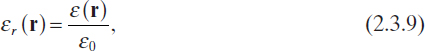
where ε₀ ≈ 8.85 × 10⁻¹² F/m denotes the dielectric permittivity of the vacuum and μ₀ = 4π × 10⁻⁷ H/m is the magnetic permeability of the vacuum. Dielectric permittivities and magnetic permeabilities are often replaced by their relative counterparts ε_r and μ_r, defined as follows:

Another important property of media is the time dispersiveness, which is essentially related to dynamics of matter polarization. In the frequency domain, time dispersiveness corresponds to complex-valued dielectric permittivities or magnetic permeabilities depending on the operating frequency.

The different microscopic mechanisms at the base of time dispersiveness can be modeled by several formulas. One of the most common is the Debye one (Balanis 1989), which states that

where ε_s and ε_∞ are the dielectric permittivities for ω = 0 and for ω → ∞, respectively, whereas τ(s) is a parameter typical of the medium called the relaxation time.

Moreover, in conducting media, an induced current is generated by the field. For a wide category of materials, Ohm's law holds, which states that the induced current density is given by

where σ(S/m) is the electric conductivity of the medium. Consequently, in the presence of a linear, isotropic, and conducting medium for which equation (2.3.12) is valid, Maxwell's equation (2.1.11) can be rewritten as

where J₀ is the impressed current density. If the effective dielectric permittivity

is introduced, equation (2.3.13) can then be written as

Accordingly, dispersive and conducting media can be treated in the same way, specifically, by using the complex-valued dielectric permittivity defined by (2.3.14). In this way only the impressed current J₀ explicitly appears in Maxwell's equations.

In several applications of microwave imaging, as will be widely discussed in the following chapters, retrieving the values of the complex dielectric permittivity of a given target or scenario often represents the objective of the reconstruction.

2.4 WAVE EQUATIONS AND THEIR SOLUTIONS

Let us consider a homogeneous medium characterized by a dielectric permittivity ε (possibly, complex-valued) and a magnetic permeability μ. By taking the curl of equation (2.1.10) and substituting the result into equation (2.1.11), one obtains

These equations, called the vector wave equations, necessitate suitable boundary conditions. Several uniqueness theorems can be derived for such a problem. For example, if the region of interest V, bounded by the closed surface S, is lossy, the tangential component assigned to S is sufficient for unique determination of the electromagnetic field inside V. The same uniqueness results hold true even if is specified on a part of S and on the other one.

The relevant conditions to be satisfied when wave equations (2.4.1) and (2.4.2) need to be solved, in an unbounded medium, are the Silver–Müller radiation conditions, which read, for , as

where is the unit radial vector and is the intrinsic impedance [in ohms (Ω)] of the medium (Van Bladel 2007).

The electromagnetic field generated in an unbounded region (free-space radiation) by the impressed source J₀ satisfying equations (2.4.1) and (2.4.2), along with the radiation conditions (2.4.3) and (2.4.4), can be expressed in integral form as

where is the free-space Green dyadic tensor given by (Tai 1971)

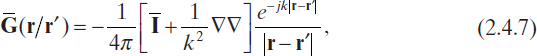
where is the wavenumber [in reciprocal meters (m⁻¹)] of the propagation medium. It is worth noting that Green's dyadic tensor is related to the radiation produced by an elementary source and provides a solution to the following tensor equation:

It is noteworthy that if r ∈ V, the integral operator of equation (2.4.5) has to be carefully dealt with because of the involved singularities of the free-space Green tensor. In fact, the correct meaning of such an integral is as follows (Van Bladel 2007)

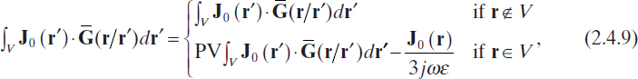
where PV denotes the principal value of the integral.

Equations (2.4.5) and (2.4.6) provide the field radiated in free space by a given bounded source. Similar expressions hold in different conditions, provided the suitable Green function is used. One of the most relevant situations for diagnostic applications consists of a source radiating in a half-space, which model, for example, the detection of objects buried in soil by using an illumination/measurement system located in air.

Without loss of generality, let us suppose that the two half-space regions are separated by the plane z = 0. We assume that the upper region (z > 0) is characterized by ε₁ and μ, whereas the lower region (z ≤ 0) is characterized by ε₂ and μ. If a bounded distribution of electric current density is present in the upper region, the electric fields in the two regions can be written as (Chew 1990)

where

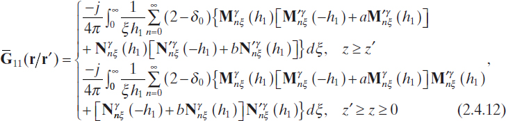
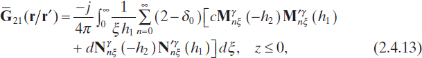
where , and δ₀ is the Kronecker delta function, such that δ₀ = 1 if n = 0, and δ₀ = 0 otherwise. In equations (2.4.12) and (2.4.13), M^γ_nξ and N^γ_nξ denote cylindrical vector functions given by (Tai 1971)

where the superscript γ indicates even (when γ = e) and odd (when γ = o) modes, so that, in equations (2.4.14) and (2.4.15) the upper symbols are valid for γ = e, whereas the lower ones hold when γ = o. Finally, the coefficients a, b, c, and d are given by (Tai 1971)

Analogous relations hold for the magnetic fields. Obviously, by suitably changing the subscripts related to the two regions, similar expressions can be derived for the field produced by a source located in the lower region. Moreover, for a multilayer structure (a model seldom used for imaging applications), similar relationships can be devised. In particular, the expression for the related Green tensor can be found in the text by Chew (1990).

It should be noted that equations (2.4.5) and (2.4.6) (free space) are also basic equations in antenna theory since an antenna can usually be modeled as a distribution of electric current. Moreover, at a great distance from the source, the following far-field approximation can be used (Collin and Zucker 1969):

This approximation is valid in the so-called far-field region, that is, for r > 10λ, r > 10d, and r > 2d²λ⁻¹, where d is the diameter of the smallest sphere, including the source and centered at the origin of the frame, and λ is the wavelength in the propagation medium. According to equations (2.4.20) and (2.4.21), in the far-field region the electromagnetic field results to be a transverse electromagnetic spherical wave. Expression (2.4.20) can also be rewritten as

Where E_∞ is a tangential vector (radiation pattern vector) given by

Moreover, from equations (2.4.20) and (2.4.21), the electromagnetic field is found to have the local characteristics of a plane wave propagating along the radial direction. In fact, the most general form of a plane wave is

where k is the propagation vector such that |k| = k, = k/k and the complex polarization vector (), which must be orthogonal to the propagation direction ( · k = 0). Plane waves are particular solutions of Mawxell's equations, which are usually considered in microwave imaging techniques to model the interrogating fields used for the exposition of the unknown targets. However, since far-field radiation conditions are seldom valid for short-range inspection techniques in the relevant frequency bands, also other source models are often adopted. One of the most common approaches consists in assuming the field generated by the transmitting antenna to be similar to that of an infinite line-current source. In this case, if the source coincides with the z axis (without loss of generality), the electric field it produces is given by (Harrington 1961)

where and denote the zero-and first-order Hankel functions of second kind, where J_n(x) and Y_n(x) are the Bessel functions of the first and second kind of nth order, respectively (Harrington 1961). Moreover, in equations (2.4.26) and (2.4.27), I denotes the complex amplitude of the current density vector J₀(r) = Iδ(ρ).

It is interesting to observe that, for large arguments, these expressions can be approximated by their asymptotic expressions as

which again show that the electromagnetic field locally behaves like a plane wave in the far-field region.

2.5 VOLUME SCATTERING BY DIELECTRIC TARGETS

In the previous sections we recalled some basic concepts of radiation. When an object—which in this context is also referred to as target or scatterer—is present in the propagation medium, the wave produced by the source interacts with it and the field distribution is affected by the presence of the scatterer. The situation is schematized in Figure 2.1, which describes a scattering configuration involving only dielectrics or materials with a finite electric conductivity.

In this context, let us assume the object to be characterized by ε and μ and immersed in a homogeneous and infinite medium (free-space scattering) characterized by ε_b and μ_b. Since the scatterer may be inhomogeneous, its dielectric parameters are in general dependent on r.

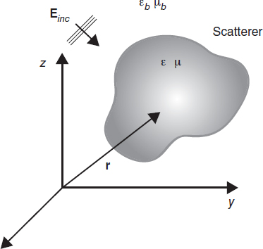
FIGURE 2.1 Electromagnetic scattering by a three-dimensional inhomogeneous target.

The perturbed field (which is the only field that can be measured in the presence of the object) is indicated by E and H. This field is clearly different from the field generated by the source when the object in not present, which is usually indicated as the unperturbed or incident field and denoted by E_inc and H_inc. The incident field is a known quantity if the source is completely characterized, and it can be computed everywhere by using relations (2.4.5) and (2.4.6). Moreover, we can write

where the difference between the perturbed field (i.e., the field when the object is present) and the unperturbed incident field (i.e., the field when the object is not present) is called the scattered field and can be ascribed to the presence of the object and, in particular, to the interaction between the incident field and the object itself. Since equations (2.5.1) and (2.5.2) can be immediately rewritten as

the perturbed fields E and H are usually indicated as the total fields.

Two situations usually occur. In the first one, the object is completely known and one has to compute the perturbed fields. This is called a direct scattering problem. For the free-space configuration in Figure 2.1, the following quantities are assumed as known quantities in the direct scattering problem: the incident fields E_inc and H_inc (for any r inside and outside the object); the values of ε_b and μ_b; the space region V_o occupied by the object; and the distributions of the dielectric parameters of the object, ε(r) and μ(r), r ∈ V_o. The goal is the computation of the scattered fields E_scat and H_scat everywhere. From these fields, one can immediately deduce the total fields E and H by using (2.5.3) and (2.5.4).

In the second situation considered, which is of paramount importance for this book, the object is unknown and one has to deduce information on it from some measurements of the perturbed field generally collected outside the object. This is called an inverse scattering problem.

For the free-space configuration considered, in the inverse scattering problem, the following quantities are still assumed known: the incident fields E_inc and H_inc (for any r inside and outside the object) and the values of ε_b and μ_b. On the contrary, V_o and the distributions of ε(r) and μ(r), r ∈ V_o, are now unknown quantities. Moreover, it is assumed that the total electric fields, E and H. are known quantities (e.g., obtained by suitable measurements) only for r ∉ V_o. In this case, the objective of the computation is the definition of the object support V_o and the reconstruction of ε(r) and μ(r), r ∈ V_o. It is evident that in practice it is impossible to measure E and H for any r outside the object, and so these vectors are usually available at a discrete set of points.

Furthermore, in certain applicative scenarios, some information about the object, referred to as a priori information, could be available. This information can be useful in limiting the space wherein the solution is searched for and to improve the reconstruction output.

With regard to practical applications, it is very important to observe that reconstruction of the complete distributions of the dielectric parameters of the unknown objects may be a of limited interest, since far fewer details may be required (e.g., in nondestructive testing, retrieving the position and/or shape of a defect in an otherwise known object could be the only information needed). Although these considerations will be discussed in the following chapters, in order to describe both the direct and inverse scattering problems in greater depth, it is necessary to deduce equations relating the measured values of the electromagnetic field to the properties of the scatterer under test. Such relations can be obtained by using the volume equivalence principle, described in the next paragraph.

2.6 VOLUME EQUIVALENCE PRINCIPLE

Let us consider the configuration shown in Figure 2.2a. Since the object actually is a discontinuity in the propagation medium, it is opportune to formulate the problem by using the integral form of Maxwell's equations. To this end, by applying equations (2.1.14) and (2.1.15), using an arbitrary open surface S whose contour is represented by a line C, for a linear isotropic medium, one obtains

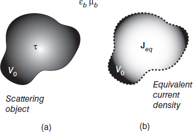
FIGURE 2.2 Volume equivalence principle. (a) real configuration; (b) equivalent problem with the equivalent current density.

Analogously, the incident field (i.e., the field when the object is not present) satisfies the following equations

Subtracting (2.6.3) from (2.6.1) and (2.6.4) from (2.6.2), yields

According to equations (2.5.1) and (2.5.2), we obtain

By introducing the equivalent sources

we can rewrite equations (2.6.7) and (2.6.8) as

The scattered field can then be considered to be generated by an equivalent electric current density and an equivalent magnetic current density, both radiating in free space. According to (2.6.9) and (2.6.10). these sources have supports coinciding with the space region occupied by the object [M_eq(r) = 0 and J_eq(r) = 0, r ∉ V_o].

Equations (2.6.11) and (2.6.12) express the volume equivalence theorem, which states that the field scattered by a real object is the same as the field produced by the equivalent current densities radiating in free space, provided that such sources are given by (2.6.9) and (2.6.10) (Fig. 2.2b). As expected, M_eq and J_eq depend on the object dielectric properties and the total internal field, which, in turn, depends on the incident field.

In this way, the scattered electric and magnetic fields can be expressed in integral form as

2.7 INTEGRAL EQUATIONS

Let us suppose now that the object of Figure 2.1 is nonmagnetic: μ(r) = μ₀, r ∈ V_o. Accordingly, M_eq(r) = 0 [equation (2.6.9)] and, on the right-hand sides of equations (2.6.13) and (2.6.14), the terms including the equivalent magnetic current density vanish. Although an expression for the scattered electric field has been deduced, the problem is not solved, since J_eq is an unknown quantity in both direct and inverse scattering problems. In the former, J_eq is unknown since E is to be computed [see equation (2.6.10)], whereas in the latter it is unknown because both E and ε are unknown functions.

Substituting equation (2.6.13) [with M_eq(r) = 0] into equation (2.5.3), we have

and, by using equation (2.6.10), we obtain

where

is the object function or scattering potential.

In the direct scattering problem, equation (2.7.2) must be solved for any r. This equation is a Fredholm linear integral equation of the second kind (Morse and Feshbach 1953), in which the only unknown is the total electric field vector E. In practical applications, a solution of this equation can be obtained only using a numerical method. The numerical resolution of the integral equation (2.7.2) consists of two stages. In the first one, equation (2.7.2) is considered for r ∈ V_o so that the internal total electric field can be computed. Afterward, the external total electric field [i.e., E(r), r ∉ V_o] can be easily obtained by computing the integral occurring in equation (2.7.2) by means of a quadrature method, since the right-hand side of (2.7.2) now involves only known functions. A more detailed description of this approach is provided in Chapter 3.

In the inverse scattering problem, E(r) is assumed to be measurable only for r ∉ V_o. In that case, equation (2.7.1) turns out to be a Fredholm linear integral equation of the first kind having the equivalent current density J_eq as an unknown. Unfortunately, as will be discussed below, knowledge of the equivalent current density generally provides only limited information about the scatterer under test. Consequently, it is usually necessary to reconsider equation (2.7.2). In this case, since the unknown quantities are E(r) and τ(r), r ∈ V_o, the equation to be solved turns out to be nonlinear (Harrington 1961).

2.8 SURFACE SCATTERING BY PERFECTLY ELECTRIC CONDUCTING TARGETS

As recalled from Section 2.2, the electromagnetic field inside a PEC object is zero and a surface current density J_S is present on the scatterer surface S according to equation (2.2.6). Moreover, when the object is illuminated by an incident field E_inc. the total electric field E outside the scatterer is still given by equation (2.5.3).

Since the presence of a PEC target does not affect the field radiated by J_S outside the scatterer (Harrington 1961), the total electric field can be written as

which, in the inverse scattering problem, represents an integral equation having S and J_S as the unknowns to be reconstructed.

REFERENCES

Balanis, C. A., Advanced Engineering Electromagnetics, Wiley, New York, 1989.

Chew, W. C., Waves and Fields in Inhomogeneous Media, Van Nostrand Reinhold, New York, 1990.

Collin, R. E. and F. J. Zucker, Antenna Theory, McGraw-Hill, New York, 1969.

Felsen, L. B. and N. Marcuvitz, Radiation and Scattering of Waves, Prentice-Hall, Englewood Cliffs, NJ, 1973.

Harrington, R. F., Time-Harmonic Electromagnetic Fields, McGraw-Hill, New York, 1961.

Jones, D. S., The Theory of Electromagnetism, Macmillan, New York, 1964.

Morse, P. M. and M. Feshbach, Methods of Theoretical Physics, McGraw-Hill, New York, 1953.

Stratton, J. A., Electromagnetic Theory, McGraw-Hill, New York, 1941.

Tai, C. T., Dyadic Green's Functions in Electromagnetic Theory, Intext, Scranton, PA, 1971.

Van Bladel, J., Electromagnetic Fields, Wiley, Hoboken, NJ, 2007.