CHAPTER THREE

The Electromagnetic Inverse Scattering Problem

3.1 INTRODUCTION

In the previous chapter, the equations governing the three-dimensional scattering phenomena involving dielectric and conducting materials were derived. A preliminary distinction between direct and inverse scattering problems has been introduced.

Since this book is devoted to microwave imaging techniques, which are essentially short-range imaging approaches, the scattering equations constitute the foundation for the formulation and the development of the various reconstruction procedures.

The inverse scattering problem considered here belongs to the category of inverse problems (Colton and Kress 1998), which includes many very challenging problems encountered in several applications, including atmospheric sounding, seismology, heat conduction, quantum theory, and medical imaging.

From a strictly mathematical perspective, the definition of a problem as the inverse counterpart of a direct one is completely arbitrary. To this end, it is helpful to recall the following well-known sentence by J. B. Keller (Keller 1976) quoted by Bertero and Boccacci (1998, pp. 1–2): “We call two problems inverses of one another if the formulation of each involves all part of the solution of the other. Often, for historical reasons, one of the two problems has been studied extensively for some time, while the other has never been studied and is not so well understood. In such cases, the former is called a direct problem, while the latter is the inverse problem.”

On the contrary, from a physical perspective, it is generally recognized that the differences between direct and inverse problems are related to the concepts of cause and effect. In the specific case considered in this book, the direct problem is related to computation of the field that is scattered by a known object (where the interaction between the incident field and the object is the cause of the scattering phenomena), whereas the inverse problem concerns the determination of the object starting from knowledge of the field scattered (the effect of the interaction).

Nowadays, inverse problems, which in the past were considered difficult and “strange” problems, have been widely studied from a mathematical perspective, and several books discuss such problems in depth (e.g., Colton and Kress 1998, Bertero and Boccacci 1998, Engl et al. 1996, Tarantola 1987, Chadan and Sabatier 1992, Herman et al. 1987, Tikhonov and Arsenin 1977).

The most critical aspect of an inverse problem is usually its ill-posedness. Following the definition by Hadamard (1902, 1923), a problem is well posed if its solution exists, is unique, and depends continuously on the data. The last property essentially means that a small perturbation of the data results in a small perturbation of the solution. If one of these conditions is not satisfied, the problem is called ill-posed or improperly posed.

In imaging applications, one measures the scattered field and tries to obtain information on the object subjected to the incident radiation. If, for a given set of measurement values (real data can be affected by noise or measurement errors), there is no object that produce the prescribed field distribution, the problem lacks in existence. Moreover, if two or more different objects produce the same measurement data, the problem solution is not unique. Finally, if two very similar sets of measurements are generated by two significantly different objects, the problem solution does not depend continuously on the data, since small errors in the measurements result in large errors in the solution.

The well-posedness of the very general problem of finding f ∈ X, given g ∈ Y, such that

where A is an operator (potentially nonlinear) mapping elements of the normed space X into elements of the normed space Y, depends essentially on the properties of the operator itself.

In particular, the problem turns out to be well posed if the operator A is bijective (i.e., injective and surjective) and the inverse operator A⁻¹ such that

is continuous. Injectivity ensures that for any g for which the solution exists, such a solution is unique (uniqueness), whereas surjectivity guarantees that there is a solution f for any g (existence). Finally, if A⁻¹ is continuous, the solution depends continuously on the data (stability). Obviously, if A does not fulfill all the requirements, described above, the problem is ill-posed.

If A is a completely continuous operator (i.e., an operator that is compact and continuous), then the problem described by equation (3.1.1) can represent an important example of an ill-posed problem. In fact, if A is such an operator, then equation (3.1.1) is ill-posed unless X is of finite dimension.

The proof of this statement (Colton and Kress 1998) can be provided as follows. Assume that A^–1 exists and is continuous. As a result, I = A⁻¹A (where I is the identity operator in the space X) is compact, since the composition of a continuous and a compact operator is also compact.

Because the identity operator is compact only if the space in which they are defined is of finite dimension, the thesis follows. We note that such a result holds true even if A is a nonlinear operator.

Ill-posedness is a very common property of inverse problems that make them very difficult to solve. Regularization procedures are useful tools in controlling ill-posedness. Applying a regularization procedure means replacing the original ill-posed problem with another well-posed problem, in which some additional information can be added. From this new problem one expects to obtain an approximate solution of the original problem. However, adding further information requires some knowledge of the behavior of the solution to the original problem. This information is usually called a priori information and can be related, in imaging applications, to the physical nature of the body to be inspected, such as its spatial extension, and/or to the noise level of the measured data.

3.2 THREE-DIMENSIONAL INVERSE SCATTERING

Let us consider Figure 3.1. According to the previous definitions, it is assumed that E can be measured for r ∉ V_o. In particular, E can be available in an observation domain V_m, which corresponds, in practical applications, to the region spanned by the measurement probes (resulting in V_m ∩ V_o = Ø). Moreover, because of the limited information content of the data, equation (2.7.2), for r ∈ V_m (hereafter called the data equation), is often solved together with the equation that provides the internal field distribution (often called the state equation). This relationship is still given by equation (2.7.2), but in this case it is valid for r ∈ V_o, So the problem solution is reduced to solving the following set of nonlinear integral equations:

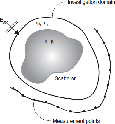
FIGURE 3.1 Imaging configuration for three-dimensional inverse scattering; investigation and observation domains.

Although formally similar, these equations are, of course, very different, since the left-hand side of equation (3.2.1) (which is a Fredholm equation of the first kind) is a known quantity, whereas the corresponding term in equation (3.2.2) (which is a Fredholm equation of the second kind) is unknown.

Formulated in this way, one can view the resolution of the inverse problem as the search for the object that produces a prescribed scattered field distribution (equal to the one that has been measured in the observation domain), but, at the same time, produces an internal field distribution consistent with the known incident field inside the object itself. It is simply the presence of the known internal field [and, consequently, the constraint imposed by the requirement of fulfilling equation (3.2.2)] that distinguishes the inverse scattering problem so sharply (also in terms of well-posedness issues) from the inverse source problem (i.e., the retrieval of a source from the field that it radiates). This point is discussed further, for example, by Bleinsten and Cohen (1977), Devaney (1978), Hoenders (1978), and Stone (1987) and in the books cited in Section 3.1.

It should also be noted that the formulation given above is based entirely on electric field integral equations (EFIEs). However, other formulations for describing the scattering phenomena are available. In microwave imaging, one of the most widely applied is the contrast source formulation (van den Berg and Kleinman 1997, van den Berg and Abubakar 2001, Abubakar et al. 2006). In such a framework, the inverse problem is still treated in its nonlinear form, but the problem unknowns are the object function and the equivalent current density [which is directly related to the internal field through equation (2.6.10)].

According to this alternative formulation, the following two integral equations are considered:

As mentioned, the problems unknowns are τ and J_eq, which vanish outside V_o.

It is also worth noting that, in several applications, the external shape of the object is known and the integration domain is therefore known. In other applications, the shape of the unknown object is itself a problem unknown. In those cases, it is natural to define an investigation domain (a test region) V_i, which by definition includes the support of the scatterer under test (V_o ⊂ V_i).

In order to retrieve the shape of the scatterer, specific methods can be used (see Chapter 5). However, as a general rule, it is possible to assume that the unknown object to be inspected coincides with the investigation domain; that is, the support of τ(r) is extended to all r ∈ V_i and the integrals in equations (3.2.1) and (3.2.2) [or in equations (3.2.3) and (3.2.4)] are defined over V_i instead of V_o. Clearly, a perfect reconstruction (i.e., a successful solution of the inverse scattering problem) would yield τ(r) = 0, for r ∈ (V_iV_o), and so it would be possible to precisely define the actual object shape.

3.3 TWO-DIMENSIONAL INVERSE SCATTERING

The scattering formulation reported in the previous section concerns three-dimensional configurations. In fact, although microwave imaging techniques can in principle be applied to three-dimensional configurations without theoretical limitations, most of the approaches proposed so far in the scientific literature are still related to two-dimensional problems. In fact, the imaging of two-dimensional structures can be simplified by means of some assumptions regarding the scatterer under test and the illumination system considered. On the contrary, fully three-dimensional approaches can still be considered as preliminary proposals. Nevertheless, in the following chapters, general formulations will be discussed in a three-dimensional framework, whereas some approaches proposed for two-dimensional configurations will be described with reference to their specific imaging modalities.

If the object to be inspected has an elongate shape with respect to the space region illuminated by the source, it can be approximated as an infinite cylinder (see Fig. 3.2). This is an assumption that should be carefully verified in each application. However, under this approximation, the cross section of the cylinder can be assumed to be independent of one of the spatial coordinates (in Fig. 3.2, the z coordinate), and we obtain

where r_t is the transversal component of r, such that (in Cartesian coordinates)

Moreover, if we assume that , that is, that the incident field is z-polarized and uniform along z [transverse magnetic incident field (TM)], for symmetry reasons both the scattered electric field and the total electric field turn out to be independent of z and z-polarized fields [i.e., ]. In this case, equation (2.7.2) can be rewritten as

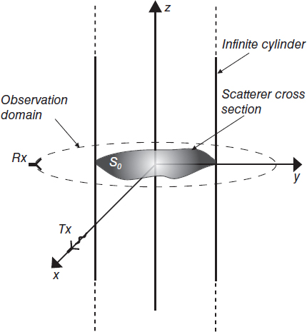
FIGURE 3.2 Infinite cylinder with an inhomogeneous cross section.

where S_o is the cross section of the cylindrical object. By using (2.4.7), we have

Moreover, since the following relation holds (Balanis 1989)

from equation (3.3.5), one obtains

or

where

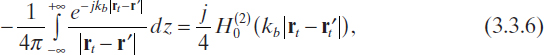
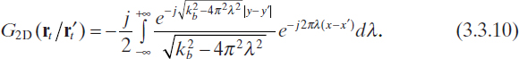
is the free-space Green function for two-dimensional problems. By using the integral representation of the Hankel function, which will be useful in development of the diffraction tomography algorithm (Section 5.2), this can also be written as (Morse and Feshback 1953)

It is important to note that these assumptions result in a greatly simplified formulation, since the inverse scattering problem turns out to be a two-dimensional scalar problem.

Furthermore, as in the three-dimensional case, the two-dimensional inverse scattering problem under transverse magnetic illumination conditions can be formulated in terms of the following two nonlinear scalar integral equations

where S_m is the observation domain (S_m ∩ S_o = Ø) where the measurements are performed. This domain is usually a circle or a segment (probing line) along which the probes are located or moved (see Chapter 4). Clearly, (3.3.11) and (3.3.12) are the two-dimensional counterparts of (3.2.1) and (3.2.2) of the three-dimensional case. Analogously, if the contrast source approach is used, the two-dimensional counterparts of equations (3.2.3) and (3.2.4) are

where

is the z component of the equivalent current density.

It should be mentioned that, when the incident field is a transverse electric (TE) field [i.e., ], the problem is still two-dimensional but the vector nature of the equations is conserved. The TE illumination has been considered by some authors (e.g., Chiu and Liu 1996 Cho and Kiang 1999, Ramananjoana et al. 2001, Qing 2002). In certain cases this illumination condition can provide better results, due to the increased information contained in the measured samples of the scattered electric field. However, the simplification inherent to the transverse magnetic illumination is partially lost.

Moreover, in exactly the same way as described for the three-dimensional case in Section 3.2, if the cross section of the object is unknown, an investigation area (a test region) S_i can be defined, which includes the cross section of the scatterer under test (S_o ⊂ S_i). In this case, the integrals in (3.3.11)–(3.3.14) are now extended to S_i instead of S_o. In this case, too, a perfect reconstruction would yield τ(r_t) = 0 for r_t ∈ (S_iS_o), allowing the definition of the object cross section.

Finally, if the infinite cylinder is a PEC one, then, under the transverse magnetic (TM) illumination condition, equation (2.8.1) can be rewritten as

where G is a closed line that determines the object profile in the transverse plane and is the contour of the object cross section in that plane. Moreover, J_sz is the z component of the surface current density J_S (see Section 2.8) and is defined on G.

3.4 DISCRETIZATION OF THE CONTINUOUS MODEL

In practical applications, the continuous model must be discretized. Several numerical methods can be applied to solve the equations involved in scattering problems. The most widely used are the method of moments (MoM), the finite-element method (FEM), and the finite-difference (FD) methods. These methods can be implemented with reference to several different schemes, and a plethora of modified and hybrid techniques can be adopted. Detailed description of these approaches is outside the scope of the present monograph, and the reader is referred to specialized books (e.g., Harrington 1968, Moore and Pizer 1984, Wang 1991, Zienkiewicz 1977, Chari and Silvester 1980, Chew et al. 2001, Mittra 1973, Press et al. 1992, Bossavit 1998, Jin 2002, Monk 2003, Taflove and Hagness 2005, Sullivan 2000, Kunz and Luebbers 1993, and references cited therein). However, for illustration purposes only, and in order to define some quantities used in the following chapters, a straightforward discretization, often used to obtain pixelated representations (images) of the original and reconstructed dielectric distributions, is presented, which is in principle based on application of MoM to a two-dimensional dielectric configuration under TM illumination. With this goal in mind, let us consider equation (3.3.8) and search for an approximate numerical solution. The problem unknowns can be expanded in a set of N basis function f_n(r_t), such that

and

In order to obtain the simplest partitioning of the investigation domain S_i, piecewise constant representations of the unknowns can be used. To this end, one chooses f_n(r_t) such that f_n(r_t) = 1 if r_t ∈ S_n, where S_n is the nth subdomain of the partitioned investigation domain (i.e., ∪_nS_n = S_i), and f_n(r_t) = 0, elsewhere. Moreover, an inner product must be introduced. Typically, for complex functions, the following product is considered (Harrington 1968)

where u and v are two generic functions of r_t having S as domain, and v* denotes the complex conjugate of v. Considering the discrete nature of the measurements in imaging applications, one can assume that the values of the scattered field are available in a set of M measurement points where the acquisition probes are located. These conditions suggest the use, as testing functions, of a set of Dirac delta functions, such that

where r_m, m = 1,..., M, is the mth measurement point. By substituting (3.4.1) and (3.4.2) in equation (3.3.8) and sequentially multiplying [by means of the inner product of equation (3.4.3)] the resulting equation by each testing function, one obtains

where

and

where E^s_m, E_m, and Eⁱ_m respectively are the z components of the scattered, total, and incident fields at the mth measurement point. In order to obtain equation (3.4.5), it has been assumed that the integral in equation (3.4.3) is extended to an infinite domain [this is clearly possible since τ(r_t) = 0 for r_t ∈ S] and the well-known properties of the Dirac delta functions have been exploited.

As a result, the problem solution is reduced to the resolution of a set of M nonlinear algebraic equations given by (3.4.5). Equation (3.4.5) can also be expressed in matrix form as

where e = [E₁,..., E_N]^T, e^s = [E^s₁,..., E^s_M]^T; [H] is a rectangular M × N matrix, whose elements are the coefficients h_mn, m = 1,..., M, n = 1,...,N; and [T] is a square N × N diagonal matrix whose diagonal elements are given by τ_n, n = 1,..., N.

It should be noted that the coefficients h_mn can be numerically computed. A very simple expression, widely used in imaging approaches and sufficiently accurate for two-dimensional TM scattering, is obtained by approximating the subdomains S_n, n = 1,..., N, by circles of equivalent areas (Richmond 1965). In this case

where a_n is the radius of the equivalent circle, ΔS_n is the area of S_n, and r_n, n = 1,..., N, is the barycenter of S_n.

As mentioned previously, the discretization procedure presented above is very simple. Various different approaches can be followed. For example, several different basis and testing functions can be used. The objective is usually to minimize the number of problem unknowns, which has a direct impact on the computational load of the method. It is also worth noting that the selected basis and testing functions are required to allow a simple computation of the coefficients and the known terms of the discretized equations.

It is also evident that the various above mentioned numerical methods can be applied not only to the two-dimensional equations considered here but also to the three-dimensional formulation of Section 3.2. A detailed example is given below. (This procedure has been applied for the numerical simulations presented thoroughout this book.) For three-dimensional scattering by isotropic dielectric bodies, the integral equation (2.7.2) can be immediately rewritten as follows (Zhang et al. 2003):

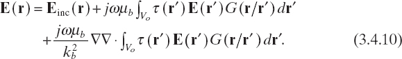
This integrodifferential equation relating the electric field and the scattering potential is often preferred to the EFIE since it avoids the problems concerning the singularities of Green's tensor (Van Bladel 2007). For development of the numerical method, it is then useful to introduce the vector field (Zhang et al. 2003)

where V_o = is assumed for convenience to be a parallelepiped containing the support of the scatterers. As a consequence, equation (3.4.10) can be written as

The first step in the implementation of the method consists in discretizing region V₀ into N = I × J × K parallelepipeds with faces parallel to coordinate directions and centers located at

for i = 1,..., I, j = 1,..., J, k = 1,..., K, where

are the lengths of the sides of the cells. In such a way, a grid of points G = i = 1,..., I, j = 1,..., J, k = 1,..., K} is introduced.

If equation (3.4.12) is enforced at each point of such a grid [i.e., Dirac delta functions located at the center of each cell are used again as testing functions (Harrington 1968)], it must hold that

where E_ijk = E(r_ijk), E^inc_ijk = E_inc(r_ijk), A_ijk, = A(r_ijk), and (∇∇ · A)_ijk is the value of ∇∇ · A evaluated at point r_ijk. In order to express (∇∇ · A)_ijk in terms of the values of A computed at r_ijk, a finite-difference scheme is used to approximate the vector differential operator ∇∇·, which in a Cartesian frame can be represented as

where

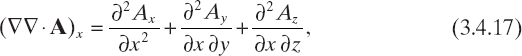
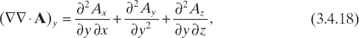
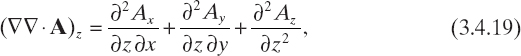
where A_x, A_y, and A_z are the Cartesian components of the vector field A.

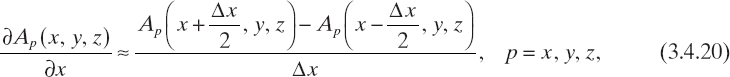
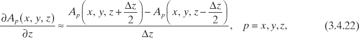
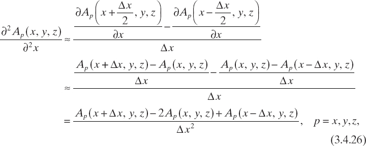
The adopted finite-difference scheme is based on two different approximations of the first-order derivatives. Namely, for computation of the second order-derivatives , p = x, y, z, the following expressions are used twice

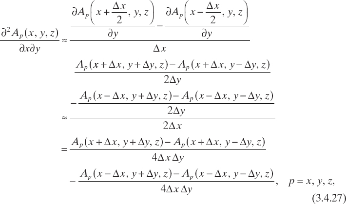
whereas the approximations used for computing the second-order mixed derivatives are as follows:

As a result, one obtains

and

and analogous relations for the other derivatives. Accordingly, the finite-difference approximation of the components of the differential operator ∇∇· can be written as

Therefore, we obtain

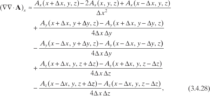
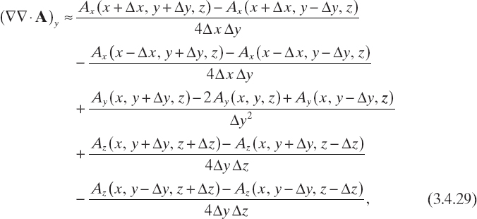
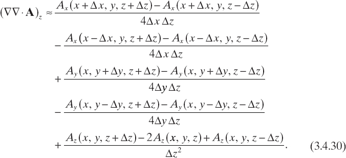
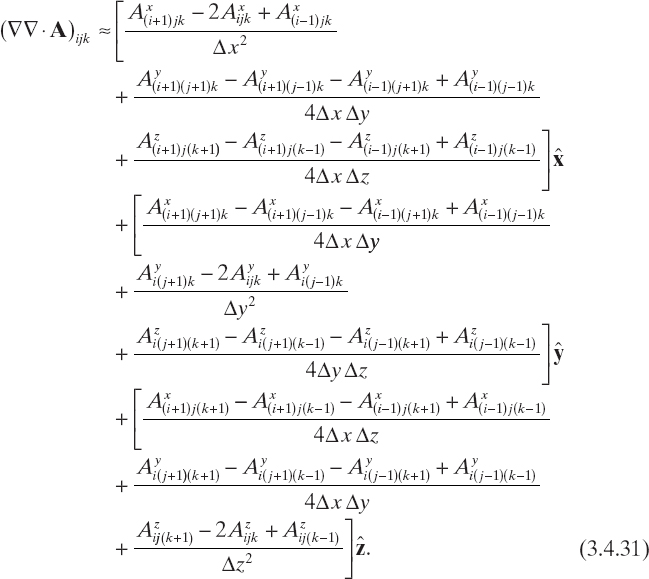
It is worth noting that, as readily follows from (3.4.31), the different finite-difference approximations (3.4.20)–(3.4.22) and (3.4.23)–(3.4.25) make it possible to express (∇∇ · A)_ijk in terms of the values of the vector field A computed on the grid points neighboring r_ijk. Equation (3.4.31) also shows that, in order to compute (∇∇· A)^ijk for i = 1,..., I, j = 1,..., J, i = 1,..., K, the vector field A has to be known on a grid containing G.

If the cells are so small that the dielectric permittivity and the electric field can be assumed to be constant over each cell, the vector field A can then be written as

for i = 0,..., I + 1, j = 0,..., J + 1, k = 0,..., K + 1, where ΔV_{i′ ,j′ ,k′} = {(x, y, z) ∈ : x₁ + (i′ − 1)Δx ≤ x ≤ x₁ + i′Δx, y₁ + (j′ − 1)Δy ≤ y ≤ y₁ + j′Δy, z₁ + (k′ − 1)Δz ≤ z ≤ z₁ + k′Δz} and τ_i′j′k′ = τ(r_i′j′k′).

It can be proved that (Zwamborn and van den Berg 1992)

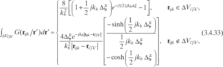
where Δξ = min{Δx, Δy, Δz}. Since the ratio in equation (3.4.33) depends on

it can be written as

As a consequence

It is noteworthy that equation (3.4.36) allows one to compute the vector field A at the points of grid G′ even if the electric field and the contrast function are known only on grid G.

With the development of a computer code in mind, it is useful to introduce an array e of 3N elements containing the values of the three Cartesian components of the electric field E on grid G. Moreover, it is very easy to check that equations (3.4.15), (3.4.31), and (3.4.36) define a linear system of equations for the elements of e. If e^inc denotes an array whose 3N entries are the three Cartesian components of the electric field E^inc on grid G, then

where [L] is a 3N × 3N matrix expressing the relationships given by equations (3.4.15), (3.4.31), and (3.4.36).

The idea underlying the numerical method described above is to solve the linear system (3.4.37) to compute the values of the electric field inside V_o and afterward to use these results to compute the electric field at any point r outside V_o. In principle, the linear system (3.4.37) can be solved by any numerical algorithm developed for linear systems, both direct and iterative. However, because of the usually enormous number of unknowns, the iterative approach is much more convenient since the particular structure of the equations involved allows for a very efficient computation of the products between matrix [L] and the solution vectors. In order to perform the simulation described, the so-called biconjugate stabilized gradient method has been applied (van der Vorst 1992, Xu et al. 2002). Following the notation by Zhang et al. (2003), the method consists in the following steps:

1. Choose a guess solution e₀ and a tolerance e >0.
2. Set

   

   

   

   

   

   

3. Choose such that

   

   and set i = 0.

4. Compute

   

   

   

   

   

   

   

   

   

   

5. If

   

then terminate and the solution is e_i. Otherwise, increment the counter i and go back to step 3. Once the array e has been determined, the electric field is known at every point of grid G. In order to compute the electric field for r ∉ V₀, the integral relation (2.7.2) can be used, without any problem concerning the proper meaning of the involved integral operator.

As a result, by exploiting the previously used approximations, the p Cartesian component of the total electric field vector, E_p(r), p = x, y, z, can be written as (Livesay and Chen 1974)

where E^q_i′j′k′ = E_q(r_i′j′k′), E_incp is the p Cartesian component of the incident field vector, and g_pq, p, q = x, y, z is the pq component of Green's dyadic tensor .

Equation (3.4.56) can be simply implemented in a numerical code, since (Livesay and Chen 1974)

where p_ijk and p_i′j′k′ are the p Cartesian components of r_ijk, and r_i′j′k′, respectively. It is worth remarking that the entries of the array e are sufficient to compute the electric field at any point outside V₀, according to (3.4.56) and (3.4.57).

Some simulation results on plane-wave scattering by a homogeneous sphere are illustrated in Figure 3.3. The sphere has a radius equal to λ/2 and is characterized by ε_r = 3.0 and σ = 0.0166 S/m. The incident field is a unit plane wave [equation (2.4.24)] with k = k₀ and . The amplitude and the phase of the total electric field have been computed in a set of M = 180 points of Cartesian components given by

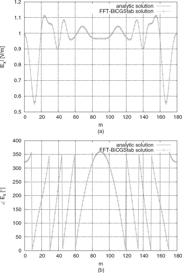
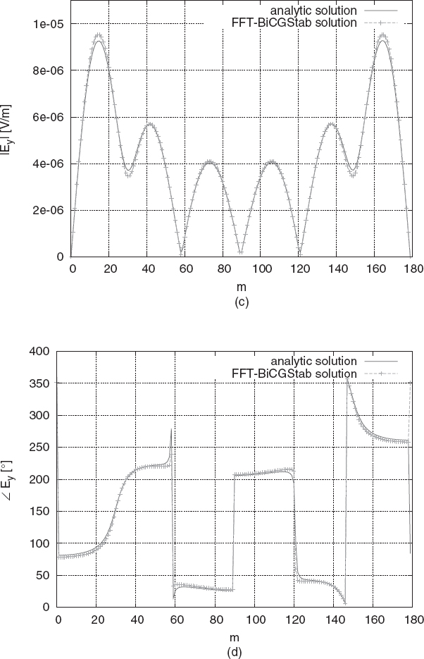
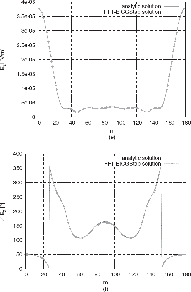
FIGURE 3.3 Scattered electric field produced by the interaction of a plane wave with a sphere (ε_r = 3.0, σ = 0.0166 S/m, radius equal to λ/2), with comparison between numerical and analytical data; total electric field (amplitude and phase): (a), (b) x component; (c), (d) y component; (e), (f) z component. (Simulations performed by G. Bozza, University of Genoa, Italy.)

Figure 3.3 plots the three Cartesian components of the total electric field. The numerical values are compared, with excellent agreement, with analytical data computed by using the eigenfunction solution for the homogeneous sphere (30 modes are considered) (Stratton 1941).

3.5 SCATTERING BY CANONICAL OBJECTS: THE CASE OF A MULTILAYER ELLIPTIC CYLINDER

As explained above, computation of the electromagnetic field scattered by arbitrarily shaped dielectric objects when they are illuminated by a generic incident field is a complex task that seldom can be performed by using analytic techniques. However, for some canonical geometries of the scatterers and for particular incident fields (e.g., plane or cylindrical waves), series expansions of the solutions for the scattered fields with analytically computable coefficients can be provided.

Among the various canonical objects reported in the literature (e.g., Stratton 1941, Bowman et al. 1969, Wait 1962), we consider here, for the sake of illustration, the scattering by a multilayer dielectric cylinder of elliptic cross section when the incident field is a plane wave polarized along the cylinder axis, that is, under TM illumination conditions (Caorsi et al. 1997a). Similar formulations can be obtained under different illumination conditions (e.g., line-current sources). A stratified elliptic cylinder is sufficiently complex to provide a good test for imaging procedures and, in general, for numerical algorithms. In fact, the assumed configuration is inhomogeneous and may contain both dielectric and conducting materials. Moreover, it does not exhibit a circular symmetry, which is an important aspect in evaluating the capabilities of tomographic imaging configurations, which are essentially based on circular geometries. In addition, elliptic cylinders are often used to approximately model several real structures, such as aircraft fuselage and other cylindrical bodies (Uslenghi 1997).

Let us consider the elliptic coordinates (u, v, z) shown in Figure 3.4. In this coordinate system, u = constant represents a family of elliptic surfaces having the same foci (located at points x = ±d on the x axis), whereas v = constant represent a family of confocal hyperbolic surfaces. Accordingly, the ith layer of the N-layer (lossless and nonmagnetic) cylinder is bounded by the elliptic surfaces u = u_i−1 and u = u_i, i = 1,..., N, with u₀ = 0. The external medium is assumed to be the free space and is denoted as the N + 1 layer. The semimajor and semiminor axes of the cylinders bounding the various layers are denoted by a_i and b_i.

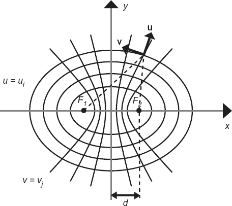
FIGURE 3.4 Elliptic coordinates for multilayer elliptic cylinders.

As mentioned previously, the illuminating field is a transverse magnetic uniform plane wave [equation (2.4.24)] with and

where φ_inc is the incident direction in the horizontal plane. The total electric field in the ith layer is given by

with i = 1,..., N, where

According to Yeh's (1963) solution, the field in the ith layer is expressed in terms of Mathieu functions, which are the eigenfunctions for the elliptic cylinder (Stratton 1941, Morse and Feshback 1953, Blanch 1965)

where ce_m and se_m denote even and odd angular Mathieu functions, Mc⁽¹⁾_m and Ms⁽¹⁾_m denote even and odd radial Mathieu functions of the first kind, Mc⁽²⁾_m and Ms⁽²⁾_m denote even and odd radial Mathieu functions of the second kind (Blanch 1965), and q_i = 0.25(k_id)², where k_i is the wavenumber of the ith layer. Finally, eⁱ_mj and oⁱ_mj, j = 1, 2 are the expansion coefficients in the ith layer (to conserve notation, we set e¹_m2 = o¹_m2 = 0).

In the external region, the electric field is the sum of the incident and scattered waves. The scattered wave can be expressed in terms of Mathieu functions of the fourth kind, Mc⁽⁴⁾_m and Ms⁽⁴⁾_m, which are analogous to the Hankel functions for the circular cylinder and can be expressed as linear combinations of the corresponding radial Mathieu functions of the first and second kinds [i.e., ]. We then obtain

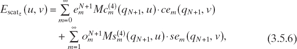
where the coefficients and depend on both the amplitude and the direction of the horizontally directed incident plane wave [see equations (2.4.24) and (3.5.1)], which, expanded in Mathieu functions, has the form

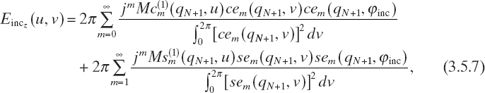
where q_N+1 = 0.25(k_bd)². The unknown coefficients can be deduced by enforcing the continuity of the tangential components of the electric field across the interfaces between layers. To this end, let us define the following quantities:

For the ith layer, by applying the Galerkin's method, one obtains

where n = 0, 1, 2,..., and

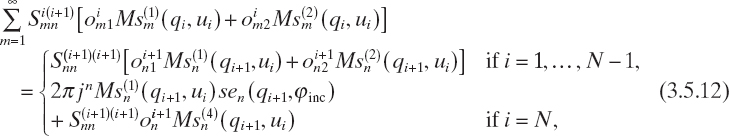
where n = 1, 2,....

Analogously, the continuity of the (u, v) component of Hⁱ(u, v) gives

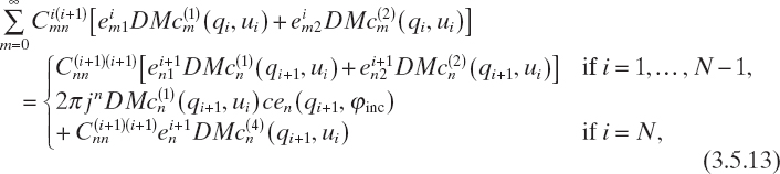
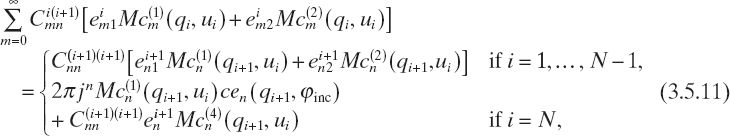
where n = 0, 1, 2,..., and

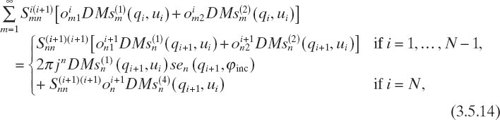
where n = 1, 2,...., and D denotes the derivatives of the Mathieu functions with respect to the u variable. To obtain these relations, we consider the fact that = 0 for any m, n, and i. Moreover, from (3.5.11)–(3.5.14), the following matrix equations can be obtained by imposing series truncations

where

and the matrices involved in (3.5.15) are block matrices given by

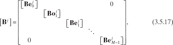
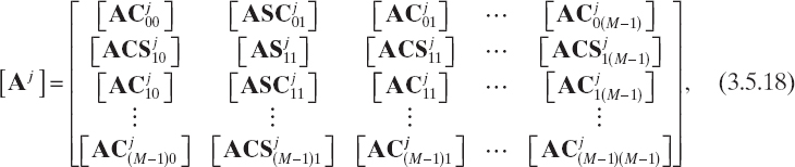
where

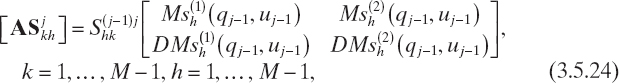
From equation (3.5.15), the coefficients of the field expansion in the (i + 1)th layer can be explicitly expressed in terms of the coefficients of the ith layer, yielding

where

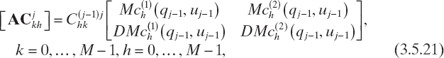
where

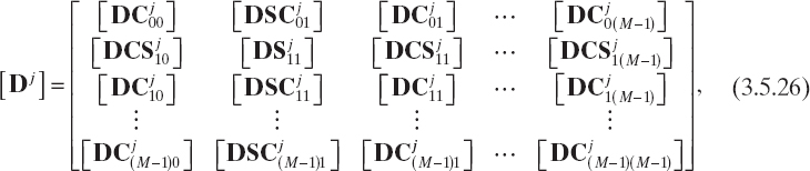
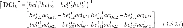
where k = 0, 1,..., M − 1, h = 0, 1,..., M − 1, and

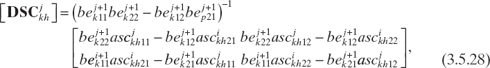
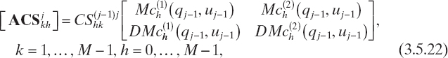
where k = 0, 1,..., M − 1, h = 1,..., M − 1, and

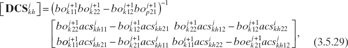
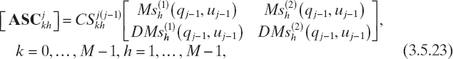
where k = 1,..., M − 1, h = 0, 1,..., M − 1, and

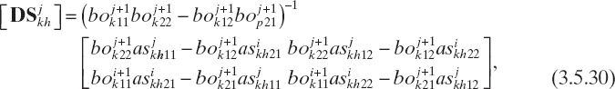
where k = 1,..., M − 1, h = 1,..., M − 1.

In equations (3.5.27)–(3.5.30), , l, p = 1, 2 indicates the elements of the lth row and pth column of matrices , and , respectively. If equation (3.5.25) is applied recursively, then, for i = 1,..., N − 1, we can obtain

where

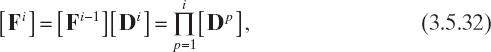
with [D⁰] = [I].

At the external boundaries, using the same procedure, we obtain analogous relations. In particular

where

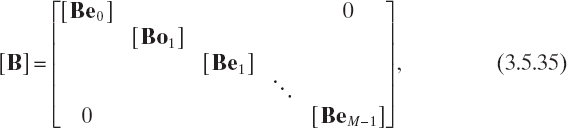
and [A^N] is as given by (3.5.18). In equation (3.5.35) the involved matrices are given by

By substituting (3.5.31) in (3.5.33), we obtain

and finally

which allows us to derive the coefficients of the external and the innermost layers simultaneously. From u^N+1 we can also deduce the far-field properties of the scattered field. In particular, the scattering width is defined as

in which the following asymptotic expression, valid for large values of u, has been applied to equation (3.5.6):

Moreover, once w¹ has been obtained from equation (3.5.33), the expansion coefficients in the other internal layers (i = 2,..., N) can be immediately obtained by using equation (3.5.25) recursively.

It should be mentioned that the recursive method described above requires the solution of only one matrix equation, exactly as does the Yeh method for a single homogeneous elliptic cylinder (Yeh 1963). Therefore, it is computationally efficient.

This procedure has been checked for several cases. Some examples are described as follows (Caorsi et al. 2000):

1. A Three-Layer Elliptic Cylinder. In this case the semimajor axes of the ellipses constituting boundaries in the transversal plane are given by a₁ = 0.1 m, a₂ = 0.16 m, and a₃ = 0.2 m (external boundary). The semifocal distance is d = 0.02 m, and the dielectric properties of the three nonmagnetic layers are ε_r1 = 2.0, ε_r2 = 1.3, and ε_r3 = 2.5, respectively. The background is vacuum (ε_b = ε₀), and the cross section center coincides with the origin of the coordinate system. The incident field is produced by a line-current source (f = 600 MHz) with unit amplitude and places on the x axis at point x = 0.505 m, y = 0.0. Figure 3.5 shows the computed total electric field (amplitude and phase) along the x and y axes obtained by using M = 10 modes for each layer. Since d is very small, the ellipses almost degenerate into circular cylinders. Consequently, the produced field can be compared with the one obtained by the eigenfunction expansion for the multilayer circular cylinder (Bussey and Richmond 1975). As can be seen, the agreement is quite good. Moreover, the same fields have been compared with the one numerically obtained by using a FEM code [with a perfectly matched layer (PML) for truncation of the domain]. Numerical codes can be used to evaluate the reliability of the procedure when the circular cylinder is not a good approximation of the scatterer under test. For the simulation reported in Figure 3.5, a square domain (including the cylinder cross section) has been considered. The side of this domain is 3m, and the discretization mesh consists of 300 × 300 equal squares, each of them divided by the positive slope diagonal. The PML used is that described by Caorsi and Raffetto (1998).
2. A Four-Layer Cylinder. In this case the simulation parameters are a₁ = 0.14m, a₂ = 0.16m, a₃ = 0.9m, a₄ = 0.2m, d = 0.12m, ε_r1 = 2.1, ε_r2 = 2.4, ε_r3 = 1.8, and ε_r4 = 1.4. The illuminating source is placed at points x = 0.505m and y = 0.305. The working frequency is again f = 600 MHz, and M = 12 modes are used. Figure 3.6 provides the results for this simulation and comparison with FEM/PML values (obtained using the same discretization as in case 1). As can be seen, the agreement is quite good, although some differences are present between the two solutions, probably due to the quite coarse mesh used for the FEM/PML computation.

   

   

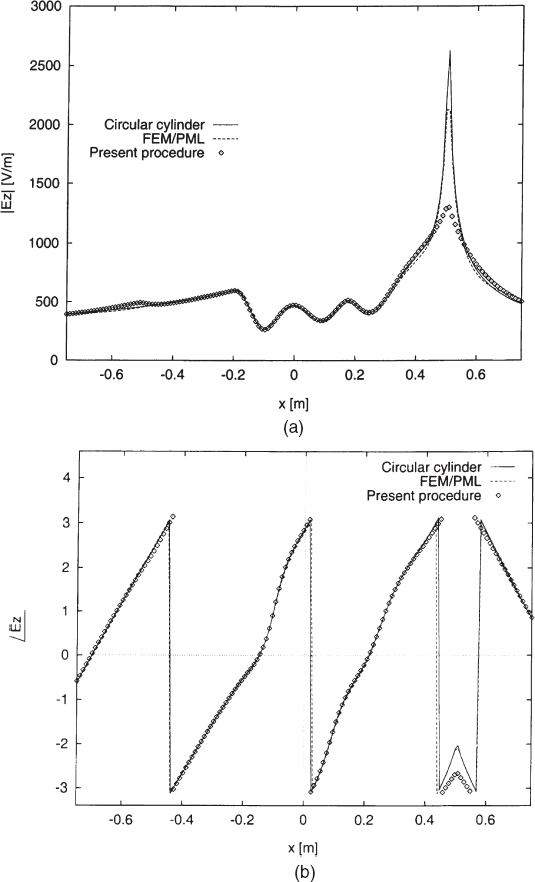
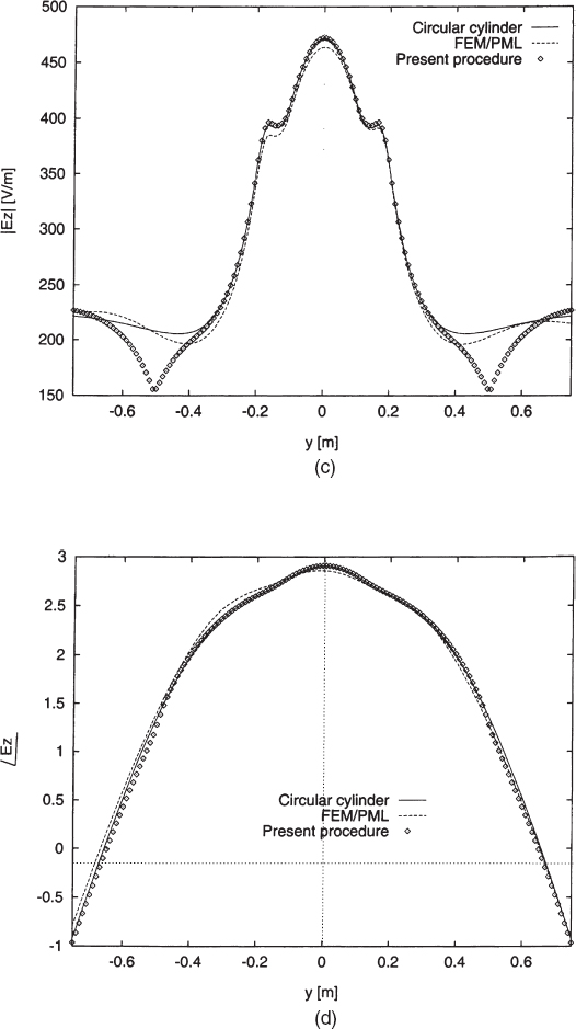
   FIGURE 3.5 Scattering by a three-layer elliptic cylinder (a₁ = 0.1m, a₂ = 0.16m, a₃ = 0.2m, d = 0.02m, ε_r1 = 2.0, ε_r2 = 1.3, ε_r3 = 2.5). Line-current source (placed at point x = 0.505m and y = 0). Working frequency f = 600MHz. Amplitude (a) and phase (b) of the total electric field computed along the x axis; amplitude (c) and phase (d) of the total electric field computed along the y axis. [Reproduced from S. Caorsi, M. Pastorino, and M. Raffetto, “Electromagnetic scattering by a multilayer elliptic cylinder under line-source illumination,” Microwave Opt. Technol. Lett. 24, 322–329 (March 5, 2000), © 2000 Wiley.]

   

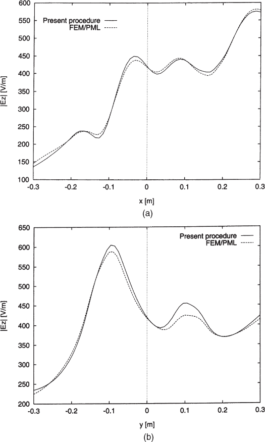
   FIGURE 3.6 Scattering by a four-layer elliptic cylinder (a₁ = 0.14m, a₂ = 0.16m, a₃ = 0.9m, a₄ = 0.2m, d = 0.12m, ε_r1 = 2.1, ε_r2 = 2.4, ε_r3 = 1.8, ε_r4 = 1.4). Line-current source (placed at point x = 0.505m and y = 0.305m). Working frequency f = 600MHz. Amplitude of the total electric field computed along the x axis (a) and the y axis (b). [Reproduced from S. Caorsi, M. Pastorino, and M. Raffetto, “Electromagnetic scattering by a multilayer elliptic cylinder under line-source illumination,” Microwave Opt. Technol. Lett. 24, 322–329 (March 5, 2000), © 2000 Wiley.]

   

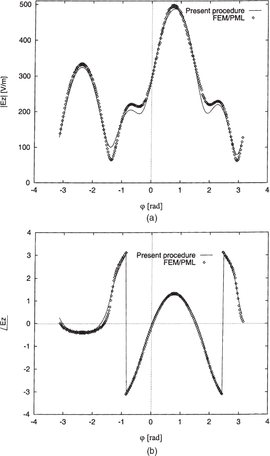
   FIGURE 3.7 Scattering by a three-layer elliptic cylinder (a₁ = 0.14m, a₂ = 0.2m, and a₃ = 0.25m, d = 0.12m, ε_r1 = 1.5, ε_r2 = 2.6, ε_r3 = 1.9). Line-current source (placed at point x = y = 0.505m). Working frequency f = 400 MHz. Amplitude (a) and phase (b) of the total electric field computed along a circle of radius R = 0.4m. [Reproduced from S. Caorsi, M. Pastorino, and M. Raffetto, “Electromagnetic scattering by a multilayer elliptic cylinder under line-source illumination,” Microwave Opt. Technol. Lett. 24, 322–329 (March 5, 2000), © 2000 Wiley.]

3. A Three-Layer Cylinder with a₁ = 0.14m, a₂ = 0.2m, and a₃ = 0.25m, d = 0.12m, ε_r1 = 1.5, ε_r2 = 2.6, and ε_r3 = 1.9. The line current is located at point x = y = 0.505m, the working frequency in this case is f = 400MHz, and M = 10 modes are used. Figure 3.7 provides the total electric field (amplitude and phase) computed along a circle of radius R = 0.4 m and centered at the origin of the coordinate system (coinciding with the center of the elliptic cross section). In this case, too, there is a very good agreement between the semianalytical data and the data obtained by using the FEM/PML numerical code.

It should be mentioned that other semianalytical solutions involving elliptic cylinders have been considered. Some examples are the simple case in which a PEC core is present (Richmond 1988, Caorsi et al. 1997b), and cases in which the multilayer cylinder consists of isorefractive materials (Caorsi and Pastorino 2004) or metamaterials (see Section 11.5) (Pastorino et al. 2005). Moreover, other similar solutions are available for other geometries, including elliptic cylinders [e.g., the case in which a PEC elliptic cylinder is coated by a circular dielectric layer (Kakogiannos and Roumeliotis 1990)].

REFERENCES

Abubakar, A., T. M. Habashy, and P. M. van den Berg, “Nonlinear inversion of multi-frequency microwave Fresnel data using the multiplicative regularized contrast source inversion,” Progress Electromagn. Res. 62, 193–201 (2006).

Balanis, C. A., Advanced Engineering Electromagnetics, Wiley, New York, 1989.

Bertero, M. and P. Boccacci, Introduction to Inverse Problems in Imaging, Institute of Physics, Bristol, UK, 1998.

Blanch, G., “Mathieu functions,” in Handbook of Mathematical Functions, M. Abramowitz and I. A. Stegun, eds., Dover, New York, 1965.

Bleinsten, N. and J. Cohen, “Nonuniqueness in the inverse source problem in acoustics and electromagnetics,” J. Math. Phys. 18, 194–201 (1977).

Bossavit, A., Computational Electromagnetics: Variational Formulations, Complementarity, Edge Currents, Academic Press, San Diego, CA, 1998.

Bowman, J. J., T. B. A. Senior, and P. L. E. Uslenghi, Electromagnetic and Acoustic Scattering by Simple Shapes, North-Holland, Amsterdam, 1969.

Bussey, H. E. and J. H. Richmond, “Scattering by a lossy dielectric circular cylindrical multilayer, numerical values,” IEEE Trans. Anten. Propag. AP-23, 723–725 (1975).

Caorsi, S. and M. Pastorino, “Scattering by a multilayer isorefractive elliptic cylinder,” IEEE Trans. Anten. Propag. 52, 189–196 (2004).

Caorsi, S., M. Pastorino, and M. Raffetto, “Electromagnetic scattering by a multilayer elliptic cylinder: Series solution in terms of Mathieu functions,” IEEE Trans. Anten. Propag. 45, 926–935 (1997a).

Caorsi, S., M. Pastorino, and M. Raffetto, “Scattering by a conducting elliptic cylinder with a multilayer dielectric coating,” Radio Sci. 32, 2155–2166 (1997b).

Caorsi, S., M. Pastorino, and M. Raffetto, “Electromagnetic scattering by a multilayer elliptic cylinder under line-source illumination,” Microwave Opt. Technol. Lett. 24, 322–329 (2000).

Caorsi, S. and M. Raffetto, “Perfectly matched layers for the truncation of finite element meshes in layered half-space geometries and applications to electromagnetic scattering by buried objects,” Microwave Opt. Technol. Lett. 19, 427–434 (1998).

Chadan, K. and P. C. Sabatier, Inverse Problems in Quantum Theory, Springer, Berlin, 1992.

Chari, M. V. K. and P. P. Silvester, eds., Finite Elements in Electrical and Magnetic Field Problems, Wiley, New York, 1980.

Chew, W. C., J. Jin, E. Michielssen, and J. Song, Fast and Efficient Algorithms in Computational Electromagnetics, Artech House, New York, 2001.

Chiu, C.-C. and P.-T. Liu, “Image reconstruction of a complex cylinder illuminated by TE waves,” IEEE Trans. Microwave Theory Tech. 44, 1921–1927 (1996).

Cho, C.-P. and Y.-W. Kiang, “Inverse scattering of dielectric cylinders by a cascaded TE-TM method,” IEEE Trans. Microwave Theory Tech. 47, 1923–1930 (1999).

Colton, D. and R. Kress, Inverse Acoustic and Electromagnetic Scattering Theory, Springer, Berlin, 1998.

Devaney, A. J., “Nonuniqueness in the inverse scattering problem,” J. Math. Phys. 19, 1526–1535, 1978.

Engl, H. W., M. Hanke, and A. Neubauer, Regularization of Inverse Problems. Kluwer Academic Publisher, Dordrecht, 1996.

Hadamard, J., “Sur les problèms aux dérivées partielles et leur significtions physiques,” Univ. Princeton Bull. 13, 49–52 (1902).

Hadamard, J., Lectures on Cauchy's Problem in Linear Partial Differential Equations, Yale Univ. Press, New Haven, CT, 1923.

Harrington, R. F., Field Computation by Moment Methods, Macmillan, New York, 1968.

Herman, G. T. et al., Basic Methods of Tomography and Inverse Problems, Adam Hilger, Bristol, UK, 1987.

Hoenders, B. J., “The uniqueness of inverse problems,” in H. P. Baltes, ed., Inverse Problems in Optics, Springer-Verlag, New York, 1978.

Jin, J., The Finite Element Method in Electromagnetics, Wiley, New York, 2002.

Kakogiannos, N. B. and J. A. Roumeliotis, “Electromagnetic scattering from an infinite elliptic metallic cylinder coated by a circular dielectric one,” IEEE Trans. Microwave Theory Tech. 38, 1660–1666 (1990).

Keller, J. B., “Inverse problems,” Am. Math. Montly. 83, 107–118 (1976).

Kunz, K. S. and R. J. Luebbers, The Finite Difference Time Domain Method for Electromagnetics, CRC Press, Boca Raton, FL, 1993.

Livesay, D. E. and K. M. Chen, “Electromagnetic fields induced inside arbitrarily shaped biological bodies,” IEEE Trans. Microwave Theory Tech. 22, 1273–1280 (1974).

Mittra, R., Computer Techniques for Electromagnetics, Pergamon Press, New York, 1973.

Monk, P., Finite Element Methods for Maxwell's Equations, Oxford Univ. Press, Oxford, UK, 2003.

Moore, I. and R. Pizer, eds., Moment Methods in Electromagnetics, Wiley, New York, 1984.

Morse, P. M. and H. Feshback, Methods of Theoretical Physics, McGraw-Hill, New York, 1953.

Pastorino, M., M. Raffetto, and A. Randazzo, “Interactions between electromagnetic waves and elliptically-shaped metamaterials,” IEEE Anten. Wireless Propagat. Lett. 4, 165–168 (2005).

Press, W. H., B. P. Flannery, S. A. Teukolsky, and W. T. Vetterling, Numerical Recipes in C: The Art of Scientific Computing, Cambridge Univ. Press, Cambridge, UK, 1992.

Qing, A., “Electromagnetic imaging of two-dimensional perfectly conducting cylinders with transverse electric scattered field,” IEEE Trans. Anten. Propagat. 50, 1786–1794 (2002).

Ramananjoana, C., M. Lambert, and D. Lesselier, “Shape inversion from TM and TE real data by controlled evolution of level sets,” Inv. Probl. 17, 1585–1595 (2001).

Richmond, J. H., “Scattering by a dielectric cylinder of arbitrary cross section shape,” IEEE Trans. Anten. Propagat. AP-13, 334–341 (1965).

Richmond, J. H., “Scattering by a conducting elliptic cylinder with dielectric coating,” Radio Sci. 23, 1061–1066 (1988).

Stone, W. R., “A review and examination of results on uniqueness in inverse problems,” Radio Sci. 22, 1026–1030 (1987).

Stratton, J. A., Electromagnetic Theory, McGraw-Hill, New York, 1941.

Sullivan, D. M., Electromagnetic Simulation Using the FDTD Method, IEEE Press, New York, 2000.

Taflove, A. and S. C. Hagness, Computational Electrodynamics: The Finite-Difference Time-Domain Method, Artech House, Norwood, MA, 2005.

Tarantola, A. Inverse Problem Theory, Elsevier, Amsterdam, 1987.

Tikhonov, A. N. and V. Y. Arsenin, Solutions of Ill-Posed Problems, Winston/Wiley, Washington, DC, 1977.

Uslenghi, P. L. E., “Exact scattering by isorefractive bodies,” IEEE Trans. Anten. Propag. 45, 1382–1385 (1997).

Van Bladel, J., Electromagnetic Fields, Wiley, Hoboken, NJ, 2007.

van den Berg, P. M. and R. E. Kleinman, “A contrast source inversion method,” Inverse Problems 13, 1607–1620 (1997)

van den Berg, P. M. and A. Abubakar, “Contrast source inversion method: State of art,” Progress Electromagn. Res. 34, 189–218 (2001).

van der Vorst, H. A., “Bi-CGSTAB: A fast and smoothly converging variant of Bi-CG for the solution of nonsymmetric linear systems,” SIAM J. Sci. Statist. Comput. 13, 631–644 (1992).

Wait, J. R., Electromagnetic Waves in Stratified Media, Pergamon Press, Oxford, UK, 1962.

Wang, J. J. H., Generalized Moment Methods in Electromagnetics, Wiley, New York, 1991.

Xu, X., Q. H. Liu, and Z. Q. Zhang, “The stabilized biconjugate gradient fast Fourier transform method for electromagnetic scattering,” Proc. 2002 Antennas and Propagation Society Int. Symp., San Antonio, Texas, USA, 614-617 (2002).

Yeh, C., “The diffraction of waves by a penetrable ribbon,” J. Math. Phys. 4, 65–71 (1963).

Zhang, Z. Q., Q. H. Liu, C. Xiao, E. Ward, G. Ybarra, and W. T. Joines, “Microwave breast imaging: 3D forward scattering simulation,” IEEE Trans. Biomed. Eng. 50, 1180–1189 (2003).

Zienkiewicz, C., The Finite Element Method, McGraw-Hill, New York, 1977.

Zwamborn, P. and P. M. van den Berg, “The three dimensional weak form of the conjugate gradient FFT method for solving scattering problems,” IEEE Trans. Microwave Theory Tech. 40, 1757–1766 (1992).