Chapter 4
Transmissions
The function of the vehicle transmission is to transfer engine power to the driving wheels of the vehicle. Changing gears inside the transmission allows matching of the engine speed and torque with the vehicle's load and speed conditions. In manual transmissions the driver must shift from gear to gear, whereas in automatic transmission the shifting is performed by a control system. There has been a gradual refinement in gearbox design over recent decades and a move towards an increasing number of gear ratios to improve overall performance and efficiency.
The chapter starts by analyzing conventional transmissions – manual gearboxes, clutches and gear ratio calculations. Then, recent developments in transmissions are reviewed and analyzed – these include Automated Manual Transmissions (AMT), Dual Clutch Transmissions (DCT) and Continuously Variable Transmissions (CVT). Their technical benefits are summarized along with the commercial issues which influence their use in current vehicle design. Two of the main trends which have influenced the increasing use of more sophisticated gearboxes have been the demands for both improved driveability and improved fuel efficiency.
Vehicles are traditionally equipped with gearboxes and differentials. The number of gears in vehicle transmissions range from three for older cars to five, six and even eight in newer ones. The differential provides a constant torque amplification ratio (final drive) and acts as a power split device for left and right wheels. The role of a gearbox is to provide different torque amplification ratios from the engine to the wheels when necessary at different driving conditions. The characteristics of IC engines were studied in detail in Chapter 2 and the torque generation behaviour of electric motors was discussed in Chapter 3. In this section, one question that will be looked at is whether with any of these torque generators, it is possible to omit the gearbox?
Consider a case in which the torque source is directly connected to a driving wheel. With reference to Figure 4.1 and ignoring the effect of rotating masses (see Section 3.9), we further assume that enough friction is available at tyre–road contact area (see Section 3.3), so the available tractive force is:
Figure 4.1 The tractive force resulting from a torque acting at the wheel centre

(4.1) ![]()
where TS and rw are the torque source and effective tyre radius respectively. For a vehicle of mass m, the acceleration resulting from this traction force is simply:
(4.2) ![]()
An accepted benchmark for the overall performance of a vehicle is the 0–100 km/h time. A guideline value for this characteristic can be considered as 10 seconds. Hence the average acceleration of the vehicle during this period is:
(4.3) ![]()
For a typical vehicle with a mass of 1000 kg and wheel radius of 30 cm, the average torque required at wheel centre will be:
(4.4) ![]()
From the discussions of Chapter 3 (e.g. Section 3.7), we found that the maximum acceleration occurs at start of motion and is up to 2–3 times the average acceleration. With a maximum acceleration of 2.5aav the maximum torque at the wheel is:
(4.5) ![]()
For a vehicle with specifications considered, an average power of 60 kW (80 hp) would be reasonable. Typical 60 kW IC engines and electric motors are compared in Table 4.1 in terms of the maximum torques they generate. Obviously for our example vehicle, compared to what is needed to produce required acceleration, all the torque sources have insufficient torque and are not suitable to be directly connected to the driving wheels. With an overall gear ratio n from the torque source to the driving wheels, torque amplification results. Values of n shown in the third column of Table 4.1 can generate the required acceleration for that specific torque source. With a final drive ratio nf of 3.5, the gearbox ratio ng is given in the last column of the table. In fact, the overall ratio is the gearbox ratio times the final drive ratio:
Table 4.1 Gear ratios for different power sources.

(4.6) ![]()
This gear ratio can produce the maximum acceleration but it is not useful as the vehicle speed increases. The vehicle speed from the kinematic relation ignoring the tyre slip (see Section 3.10) is:
in which ![]() is the speed of the power source. For our example vehicle equipped with an SI engine for a maximum speed of 6000 rpm, the maximum vehicle speed at overall ratio of 15 will be 45 km/h. Thus, in order to operate at higher speeds, the gear ratio must be reduced. The kinematic limitation explained above makes several gear reductions necessary during vehicle acceleration to its final speed. The gearbox is, therefore, required for this purpose. For electric motors it is possible to have no additional gear ratio and a single ratio can be used. For example, with a maximum speed of 8000 rpm and with a single gear ratio of 5, a speed of 180 km/h can be reached.
is the speed of the power source. For our example vehicle equipped with an SI engine for a maximum speed of 6000 rpm, the maximum vehicle speed at overall ratio of 15 will be 45 km/h. Thus, in order to operate at higher speeds, the gear ratio must be reduced. The kinematic limitation explained above makes several gear reductions necessary during vehicle acceleration to its final speed. The gearbox is, therefore, required for this purpose. For electric motors it is possible to have no additional gear ratio and a single ratio can be used. For example, with a maximum speed of 8000 rpm and with a single gear ratio of 5, a speed of 180 km/h can be reached.
Vehicle motion in different conditions is governed by the way power is transmitted from its source to the wheels. Gearbox ratios must be designed to match the vehicle motion with the torque generator's characteristics. In the case of an IC engine, the diverse working conditions of the engine make it very important to have proper gear ratios for good overall performance of the vehicle. Low gears are used at low speeds and should provide high tractions for accelerating and hill climbing. High gears, on the other hand, are used at higher speeds and must allow proper matching between engine torque-speed characteristics with vehicle acceleration and speed. Since the requirements for the lowest and highest speed gears are totally different, each will be considered separately.
4.3.1 Lowest Gear
The first or the lowest gear is used when highest acceleration is needed, or when the road load is high, such as on a slope. Since the gear ratio amplifies the engine torque, a large ratio will produce large wheel torques. With reference to the discussions in Section 3.3, however, the tractive force generated by a tyre is limited. Hence, increasing the gear ratio is limited by the tyre–road friction characteristics. Using Equation 3.22 for the tractive force including the driveline efficiency ![]() is:
is:
Assuming the limitation for the tractive force is, say, FTmax, the overall gear ratio nL for the lowest gear can be written as:
(4.9) ![]()
Referring to Figures 3.14 and 3.15, the maximum tractive force can be written as:
where ![]() is the maximum coefficient of adhesion in tyre–road interface and
is the maximum coefficient of adhesion in tyre–road interface and ![]() is the load on the driving axle. Thus:
is the load on the driving axle. Thus:
In order to find the axle load, consider the free body diagram of a vehicle travelling on a road of slope θ shown in Figure 4.2. The equations of motion in the longitudinal and vertical directions are:
Figure 4.2 Free body diagram of vehicle

(4.13) ![]()
where Ff and Fr are front and rear tractive forces, FA and FRR are aerodynamics and rolling resistance forces and W is the vehicle gravitational force (weight). The aerodynamic force is acting at a height of hA whereas the vehicle centre of mass is located at height h. Taking moments about the contact point of the rear wheel (point C) results in:
Combining Equations 4.12--4.14 leads to:
where:
(4.17) ![]()
(4.18) ![]()
Since ![]() is usually small, and at low speeds the aerodynamic force is also small, the last terms in Equations (4.15) and 16 can be ignored. Nf and Nr are the axle loads at the front and rear respectively. For a front wheel drive (FWD) vehicle, only Ff will br present and for a rear wheel drive (RWD), only Fr will be present. For a four-wheel drive (4WD) vehicle both tractive forces at front and rear will be acting. The axle loads in Equations (4.15) and 16 are still dependent on the total tractive force FT as can be seen. Assuming the tractive force has its maximum limiting value proportional to the axle load, substituting from Equation (4.10) into Equations (4.15) and (4.16) for FWD and RWD vehicles will result in:
is usually small, and at low speeds the aerodynamic force is also small, the last terms in Equations (4.15) and 16 can be ignored. Nf and Nr are the axle loads at the front and rear respectively. For a front wheel drive (FWD) vehicle, only Ff will br present and for a rear wheel drive (RWD), only Fr will be present. For a four-wheel drive (4WD) vehicle both tractive forces at front and rear will be acting. The axle loads in Equations (4.15) and 16 are still dependent on the total tractive force FT as can be seen. Assuming the tractive force has its maximum limiting value proportional to the axle load, substituting from Equation (4.10) into Equations (4.15) and (4.16) for FWD and RWD vehicles will result in:
The coefficient of rolling resistance is:
(4.21) ![]()
Substituting Equations (4.19) and (4.20) into Equation (4.11) will result in:
nL is the largest gear ratio and its maximum value is found at zero slope θ = 0. Equations (4.22) and (4.23) can be rearranged as:
in which F/R stands for F or R for FWD or RWD respectively, and:
Equation (4.24) can be used to calculate the largest gear ratio, however, the value of Te must be available. In fact, the engine torque does not have a constant value and it depends on the engine speed and throttle position (see Section 3.2.1). In order to find a suitable value for engine torque, let us rewrite Equation (4.24) as:
The left-hand side is the traction force resulting from the engine torque and the right-hand side expression is the limiting value for the tractive force due to the tyre–road friction. Since the maximum tractive force on the left is generated at the maximum of engine torque, therefore in Equation (4.24) the maximum of engine torque is used. If a gear ratio larger than that obtained from Equation (4.24) is used, the tyres will slip at maximum engine torque, nevertheless it is common practice to use a value of 10–20% larger. This will allow maximum tyre traction to be generated at lower engine torques. This is more practical since to gain maximum traction, it is not necessary to have a full throttle.
Example 4.3.1
For a vehicle with the information given in Table 4.2:
Table 4.2 Vehicle information of Example 4.3.1
| Tyre rolling radius | 0.30 m |
| Coefficient of rolling resistance | 0.02 |
| Engine maximum torque @ 2800 rpm | 120 Nm |
| Vehicle mass | 1200 kg |
| Maximum road adhesion coefficient | 0.9 |
| Weight distribution F/R | 58/42% |
| CG height to wheelbase ratio h/l | 0.30 |
| Driveline efficiency | 85% |
(a) Calculate the low gear ratio for both cases of FWD and RWD.
(b) For front/rear weight distributions 60/40, 55/45 and 50/50 vary the road adhesion coefficient from 0.5 to 1.0 and plot the ratio of kR to kF.
(c) For the weight distribution of case (b), plot the variation of gear ratios versus variation of μp from 0.7 to 1.0.
Solution
For (a), from row 6 of Table 4.2, a/l = 0.42 and b/l = 0.58. From Equation (4.25):
![]()
![]()
![]()
![]()
For (b), a simple MATLAB® program can generate the results. The output plots are shown in Figure 4.3. It is clear that kR is greater than kF at most practical cases.
Figure 4.3 Variation of ratio kR/kF with adhesion coefficient μp

For (c), the plot is shown in Figure 4.4. As can be seen for RWD, the vehicle gear ratios are larger, which implies that under similar road conditions, larger traction forces can be produced at the rear wheels. It should be noted that this result is due to dynamic conditions when the vehicle accelerates or on slopes where the load transfer from front to rear takes place. The difference between FWD and RWD layouts increases with increasing a/l ratio.
Figure 4.4 Variation of overall gear ratio with adhesion coefficient μp

4.3.1.1 Gradability
The maximum grade a vehicle can negotiate depends on two factors: first, the limitation of road adhesion and, second, the limitation of the engine torque. In order to consider the limitation of road friction, the right-hand side of Equation (4.26) with the inclusion of the slope angle, dictates the maximum traction force:
(4.27) ![]()
and this must overcome the resistive forces FR,
(4.28) ![]()
Assuming the vehicle moves at low speed, then the aerodynamic force will be negligible. Thus for a constant speed of travel on a slope θ we have:
(4.29) ![]()
or the maximum slope travelable for the vehicle is:
The limitation of the engine torque is not in general critical to gradeability as it is always possible to increase the gear ratio to increase the tractive force. If the torque is limited, the left-hand side of Equation (4.26) dictates the maximum traction force. At low speeds:
which can be solved for θ. The minimum of the values obtained from Equations (4.30) and (4.31) will be the gradeability of the vehicle at low speeds.
Example 4.3.2
For the vehicle of Example 4.3.1:
(a) Determine the climbable slope for both cases of FWD and RWD.
(b) Plot the variation of gradable slopes with the variation of μp at different a/l ratios (use the road friction limitation).
Solution
(a) For a FWD vehicle from Equation (4.30), the slope angle can be determined using the information from the previous example:
![]()
If the torque limitation is imposed, the result from Equation (4.31) will be:
![]()
For the RWD case, the result is: ![]() , or, θ = 26.12 deg. for the limitation on friction. The torque limitation results:
, or, θ = 26.12 deg. for the limitation on friction. The torque limitation results: ![]() with θ = 29.5 deg. Therefore the grading angle for FWD is 21.55 deg. and for RWD it is 26.12 deg.
with θ = 29.5 deg. Therefore the grading angle for FWD is 21.55 deg. and for RWD it is 26.12 deg.
(b) Gradable slopes plotted in Figure 4.5 show that RWD vehicle has better gradeability for different designs over roads with given coefficients of adhesion.
Figure 4.5 Gradable slopes versus the adhesion coefficient at different weight distributions

4.3.2 Highest Gear
The highest gear is usually used for cruising at high speeds. The maximum vehicle speed is attained at the top gear as a result of the dynamic balance between the tractive and resistive forces (see Section 3.7.4). From the kinematic point of view, the maximum speed of a vehicle in the highest gear nH will occur at a certain engine speed ![]() so:
so:
If the tyre slip ![]() is also taken into account (see Section 3.3), the modified equation will be:
is also taken into account (see Section 3.3), the modified equation will be:
For a target top speed of vmax if ![]() was known, the gear ratio nH could simply be calculated. However,
was known, the gear ratio nH could simply be calculated. However, ![]() is the result of the power balance between the engine and resistive forces which is dependent on the design parameters including the gear ratio.
is the result of the power balance between the engine and resistive forces which is dependent on the design parameters including the gear ratio.
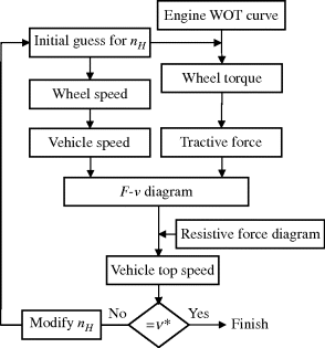
The highest gear in the gearbox (e.g. 5th) sometimes is designed by assuming ![]() to be about 10% higher than the engine speed at the point of maximum engine power, then the final gear is designed by arranging it to be an overdrive (see Section 4.3.2.2) of up to 30% [1]. For the design of the highest gear, it is reasonable to consider a full throttle condition for the top speed of vehicle, therefore the WOT curve of engine can be used to find the dynamic balance point. In general, as Figure 4.6 illustrates, the intersection of the tractive and resistive force diagrams defines the balance point at which a steady state condition results and the vehicle speed will remain constant.
to be about 10% higher than the engine speed at the point of maximum engine power, then the final gear is designed by arranging it to be an overdrive (see Section 4.3.2.2) of up to 30% [1]. For the design of the highest gear, it is reasonable to consider a full throttle condition for the top speed of vehicle, therefore the WOT curve of engine can be used to find the dynamic balance point. In general, as Figure 4.6 illustrates, the intersection of the tractive and resistive force diagrams defines the balance point at which a steady state condition results and the vehicle speed will remain constant.
Figure 4.6 Top speed of vehicle at the balance point

The variation of tractive force can be written as (Equation (4.8)):
in which Te(ωe) is the engine WOT curve. Since the vehicle speed is related to the engine speed by the kinematic relation (Equation (4.32) or (4.33)), the variation of tractive force with speed can be obtained. Equation (4.34) indicates that the tractive force is dependent on the gear ratio nH, thus without knowing it, the tractive force cannot be constructed. If the design value of the top speed (say, v*) is given, an iterative procedure starting with an initial value for nH can be used, the tractive and resistive forces can be constructed and the intersection of the two curves gives the top speed. If this value is equal to v*, the initial guess for nH is correct, otherwise its value should be modified and the procedure repeated. The flowchart of Figure 4.7 illustrates this procedure.
Figure 4.7 Flowchart to obtain nH
An alternative and somewhat simpler approach is also available to calculate the highest gear. According to the resistive force diagram of Figure 4.8, at a specified top speed of v* the resistive force has a value F* which is also equal to the tractive force at this point. Therefore, with known values for the tractive force and the top speed, the required power P* will also be known:
Figure 4.8 The tractive force is equal to the resistive force at the final speed

This power also includes the driveline losses (see Section 3.13) and the engine provides the total power sum P*. In the engine WOT power-speed curve, a horizontal line at P* value intersects the curve and gives an engine speed ![]() (see Figure 4.9). Then, from Equation (4.32) (or 4.33), the high gear ratio nH can simply be obtained.
(see Figure 4.9). Then, from Equation (4.32) (or 4.33), the high gear ratio nH can simply be obtained.
Example 4.3.3
A vehicle with mass of 1000 kg, overall aerodynamic coefficient of 0.35 and tyre rolling radius of 30 cm, has an engine WOT torque-speed formula of the form:
![]()
in which ![]() is in rpm. The intention is to have a top speed of 180 km/h for the vehicle. Design the high gear ratio, if the coefficient of rolling resistance is 0.02. Ignore the driveline losses and tyre slip.
is in rpm. The intention is to have a top speed of 180 km/h for the vehicle. Design the high gear ratio, if the coefficient of rolling resistance is 0.02. Ignore the driveline losses and tyre slip.
Solution
The total resistive force and power at the top speed are:
![]()
![]()
The engine speed for this power can be obtained by solving the equation:
![]()
The term ![]() is necessary to convert the
is necessary to convert the ![]() term to rad/s. The solution can be found by trial and error or by using MATLAB function ‘fsolve’. The result is
term to rad/s. The solution can be found by trial and error or by using MATLAB function ‘fsolve’. The result is ![]() . The overall gear ratio then can be found by using Equation (4.32).
. The overall gear ratio then can be found by using Equation (4.32).
![]()
Figure 4.9 Finding the engine working speed at the top speed of the vehicle

4.3.2.1 Design for Maximum Speed
The standard resistive force/power curves for a given vehicle are fixed in the F-v or P-v relationships. The tractive force/power curves, however, vary with the gear ratio (Equation (4.8)). The dynamic balance points, therefore, will also vary with the variation of the high gear ratio. Figure 4.10 illustrates the variation of traction/power diagrams and the resulting top speed points with the variation of the gear ratio. It shows that the maximum top speed is achievable at the maximum power point. Other top speeds at the points where the tractive and resistive force/power diagrams intersect are lower than this maximum value. In other words, there is one gear ratio for which the top speed is attained at the maximum power of engine and this speed is the maximum speed achievable.
Figure 4.10 Traction/power diagrams, the variation of top speed with change of gear ratio

Mathematically, at the balance point, according to Equation (4.35):
which simply shows that the top speed vtop is maximum where the power P* is maximum. This belongs to a certain gear ratio ![]() and if this ratio is either increased or decreased, the maximum speed will be reduced. Figure 4.11 shows this effect for two larger and smaller ratios which have similar final speeds.
and if this ratio is either increased or decreased, the maximum speed will be reduced. Figure 4.11 shows this effect for two larger and smaller ratios which have similar final speeds.
Example 4.3.4
For the vehicle in Example 4.3.3, find the gear ratio in order to achieve the maximum possible speed.
Solution
The maximum power point can be found from the full throttle torque-speed equation of the engine. Mathematically from:
![]()
or from numerical solutions one obtains:
![]()
From Equation (4.36):
![]()
The steady-state speed is:
![]()
Finally Equation (4.32) results in:
![]()
Figure 4.11 Reduction of maximum speed with changing gear ratio![]()

4.3.2.2 Overdrive
In Figure 4.11 it can be seen that the top speed was reduced for gear ratios smaller or larger than ![]() . When
. When ![]() is larger than
is larger than ![]() (dash-dotted curves), the top speed will occur at higher engine speeds. This will force the engine to work at fuel-inefficient points (see Chapter 5). On the other hand, when
(dash-dotted curves), the top speed will occur at higher engine speeds. This will force the engine to work at fuel-inefficient points (see Chapter 5). On the other hand, when ![]() is smaller than
is smaller than ![]() (dotted lines), the engine speed will be lower while the top speed could still be similar to the case of Figure 4.11. This is called overdrive and will move the engine working points to fuel-efficient regions as well as reducing engine noise for passengers. The term ‘overdrive’ indicates that the transmission output turns with higher speed than the engine speed. The amount of overdrive is chosen in different cars depending on other design and intended operating usage conditions. A value of 10–20% appears to be a typical practical design [2]. In mathematical form, a 10% overdrive results in:
(dotted lines), the engine speed will be lower while the top speed could still be similar to the case of Figure 4.11. This is called overdrive and will move the engine working points to fuel-efficient regions as well as reducing engine noise for passengers. The term ‘overdrive’ indicates that the transmission output turns with higher speed than the engine speed. The amount of overdrive is chosen in different cars depending on other design and intended operating usage conditions. A value of 10–20% appears to be a typical practical design [2]. In mathematical form, a 10% overdrive results in:
Example 4.3.5
For the vehicle in Example 4.3.4, design a 10% overdrive high gear.
Solution
According to Equation (4.47):
![]()
It can be observed from comparing this result with the result of Example 4.3.3 (with nH = 3.13) that a 10% overdrive has not significantly altered the top speed of vehicle notably (181 km/h has become 180) whereas the engine speed has reduced considerably from 5500 rpm to slightly below 5000 (about 10%).
4.3.2.3 Reserve Power
With an overdrive, the maximum power of the engine is not available for use in the high gear since the force balance is achieved below the maximum power. For reasons of providing better vehicle performance at the times when an extra load is acting (like a head wind or a slope), it is useful to keep some reserve power to be utilized at such circumstances. An obvious solution is to have the installed power of the engine greater than the designed power. With a greater installed power, the reserve power and tractive force will be increased but the maximum speed of the vehicle will also increase.
In practice, at any working speed, extra traction and power are available at a larger gear ratio. For example, the dotted curve of Figure 4.12 represents gear ratio A which is larger than the gear ratio B shown in the solid curve but both gears have an equal maximum speed. At a specific speed (e.g. 120 km/h), the reserve power and tractive force are greater for gear A. If the vehicle needs a greater acceleration capability even at its high gear (like a sports car), then this type of gear ratio design would be preferred. In a passenger car, however, an overdrive (e.g. gear B) is more appropriate and in practice when the load is high, a downshift could provide more reserve power and tractive force during vehicle motion. In this case, the gear A can be regarded as 4th gear and the gear B as the 5th gear. Further considerations are also needed for the design of the high gear. One good approach, for example, is to have enough torque and traction in the high gear to be able to maintain it at lower speeds. In other words, having the largest possible speed span at the highest gear makes the driving more comfortable and pleasant.
Figure 4.12 Power and tractive force reserves

4.3.3 Intermediate Gears
The gear ratio of the gearbox is the mechanism by which the vehicle and engine speeds are kinematically related. For stepped ratio transmissions, moving from a high gear to a low gear or vice versa must be carried out by shifting through the intermediate gears. By ignoring the tyre slip (Equation (4.7)):
(4.38) ![]()
For different gear ratios this relation expresses a family of lines with slopes equal to the n/rw a ratio as shown in Figure 4.13. In each gear, the variation of engine speed with vehicle speed is prescribed by its relevant line. When the gear is shifted, the working point moves on to another point on another line but at the same vehicle speed.
Figure 4.13 Kinematic relation between engine and vehicle speeds

During a gearshift, the torque transmission is interrupted by the clutch action and the engine speed starts to fall. When a new gear is engaged, the engine speed is changed to a new value (in an upshift to a lower speed and in a downshift to a higher speed). In practice, during the shift, the vehicle speed will be reduced slightly under the action of resistive forces and in the absence of the tractive force. Therefore, during an upshift or a downshift, as Figure 4.14 illustrates, the engine and vehicle speeds must move from point 1 to point 2. The location of point 2 depends on the shifting speed. If the shift is carried out slowly, the engine speed will drop further and vehicle speed will also reduce more.
Figure 4.14 Upshift and downshift in an engine-vehicle speed diagram

For a vehicle under normal driving conditions, a standard shift will take a certain time. Knowing this time period, point 2 can be located and the gear ratio can be determined from the slope of a line from origin to that point. With the selected gear ratio and a standard shift, the kinematic relation will be re-established and the engine and vehicle speeds will match exactly. Conversely, if a different shifting is carried out, the point 2 will depart from the designed location and a mismatch will occur between the engine and vehicle speeds. This is accommodated by the clutch slip and the engine is gradually adjusted to the relevant speed. For initial design values, there are standard methods for the determination of intermediate gears that will be discussed in the coming sections.
4.3.3.1 Geometric Progression Method
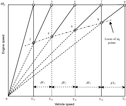
This method represents an ideal case in which the gearshift takes place at a constant speed. In addition, it is assumed that there is an engine working range between a high engine speed ωH and a low engine speed ωL as shown in Figure 4.15. According to this figure, for a 5-speed gearbox, at points 1 and 2 the kinematic relations are:
(4.39) ![]()
(4.40) ![]()
Figure 4.15 Geometric progression speed diagram

As a result:
(4.41) ![]()
Repeating the same procedure for points 3 and 4 leads to:
(4.42) ![]()
and for all ratios, one writes:
in which ![]() is the geometric progression constant and has a typical value of around 1.5. Multiplying the equalities in Equation (4.43) results in:
is the geometric progression constant and has a typical value of around 1.5. Multiplying the equalities in Equation (4.43) results in:
(4.44) ![]()
or:
(4.45) ![]()
In general, for an N-speed gearbox:
(4.46) ![]()
and from Equation (4.43):
It should be noted that ωH and ωL are only dummy variables and are not involved in the final results.
Example 4.3.6
For the vehicle in Example 4.3.3, use the low gear ratios of Example 4.3.1 and determine the intermediate gear ratios for a five-speed gearbox.
Solution
From the results of Examples 4.3.1 and 4.3.3, we have:
For a FWD vehicle: ![]() and
and ![]() , hence:
, hence:
![]()
For a RWD vehicle: ![]() and
and ![]() , therefore:
, therefore:
![]()
4.3.3.2 Progressive Design
The geometric progression method produces larger speed ranges (ΔVs) for higher gears and smaller speed ranges for lower gears, as can be seen in Figure 4.15. In mathematical form, the ratio of the speed range can be represented as:
(4.48) ![]()
In the traction-speed curves, the ratio of differences in tractive forces at three consecutive gears also follows a similar pattern:
In passenger cars it is desirable to provide larger traction differences at low gears and smaller differences at high gears. In the speed diagram this will have opposite effect of reducing the differences in speed ranges.
In the geometric progression pattern of Equation (4.43), the ratio of any two consecutive gears was a constant. If the tractive force difference ratio of Equation (4.49) is changed for different gears, then the ratio of any two consecutive gears will be different:
(4.50) ![]()
In the progressive design, the consecutive ratios Ci are related by a constant factor k:
Multiplication of the ratios Ci together equals the ratio of first to the last gear, that is:
Substituting from Equation (4.51) and after simplification results in:
(4.53) ![]()
This can be solved for C1:
(4.54) ![]()
For a five-speed gearbox, it reduces to:
Values for other Ci can be calculated by using Equation (4.51). The lowest and highest gear ratios are available and other gear ratios can be determined once the values of Ci have been calculated. In terms of the lowest gear:
(4.56) ![]()
or in terms of the highest gear:
The design can now be completed if the factor k is known. A value of k = 1 provides a geometric progression and for values less than unity, a progressive design is achieved. Small variations in k have large effects on the speed range of each gear as Figure 4.16 illustrates for a five-speed gearbox. Reducing the value of k results in the reduction of gear ratios (slopes of inclined lines) in a non-linear fashion. For example, for k = 0.8, the last ΔV becomes very small.
Figure 4.16 Speed diagram for different values of k

In the traction-speed diagram of Figure 4.17, two cases of k = 1.0 (geometric) and k = 0.9 (progressive) have been compared in terms of tractive force distribution for the gears of a five-speed gearbox. As is clear, the differences between ΔFs of the two methods at gears 1–2 and 4–5 are large but at gears 2–3 and 3–4 are close to one another.
Figure 4.17 Traction-speed diagrams for geometric and progressive designs

Values of k below 0.8 will place the 4th gear very close to gear 5 in a five-speed gearbox as seen in Figure 4.16; this is not practical, thus the working range for k can be considered as:
(4.58) ![]()
In contrast, with the geometric progression method in which a low engine speed line was present in the speed diagram for all gears, for the progressive method, each gear will have a certain low speed point as shown in Figure 4.18. The locus of ωL points is an ascending curve (close to a line) and indicates that shifting time is decreasing with gear number increase.
Example 4.3.7
Determine the progressive intermediate gear ratios for the vehicle in the previous example using k = 0.9.
Solution
For a FWD vehicle we have: ![]() and
and ![]() , and
, and ![]() . From Equation (4.55):
. From Equation (4.55): ![]()
Other C ratios are calculated from Equation (4.51):
![]()
Equation (4.57) will be used to determine the intermediate gear ratios:
![]()
For a RWD vehicle we have: ![]() and
and ![]() and
and ![]() thus:
thus:
![]()
Figure 4.18 Speed diagram for progressive gear ratios
4.3.3.3 Equal ΔVs
One particular type of progressive gear ratio selection is to set all ΔVs equal. With reference to Figure 4.18:
(4.59) ![]()
The velocities Vi of points i using a kinematic relation is:
(4.60) ![]()
Equating the first two ΔVs results in:
(4.61) ![]()
or,
and from next equality:
(4.63) ![]()
It can be proven that the general relation is:
(4.64) ![]()
The ratio Ci therefore is:
(4.65) ![]()
It is a simple task to show that:
(4.66) ![]()
Further manipulation gives:
Application of Equation (4.52) with substitution from Equation (4.67) leads to the following relation for C1:
(4.68) ![]()
That can provide an equation for n2:
(4.69) ![]()
Then in general, any of gear ratios can be obtained from:
(4.70) ![]()
Noting that ![]() , for a five-speed gearbox, the intermediate gear ratios can be found as:
, for a five-speed gearbox, the intermediate gear ratios can be found as:
Example 4.3.8
Determine the intermediate gear ratios for the vehicle in the previous example using the Equal ΔV progressive method.
Solution
For a FWD vehicle we have: ![]() and
and ![]() . From Equation (4.71):
. From Equation (4.71):
![]()
Other gear ratios are calculated similarly:
![]()
For a RWD vehicle we have: ![]() and
and ![]() and intermediate gear ratios will be:
and intermediate gear ratios will be:
![]()
Table 4.3 Some vehicle performance measures.
4.3.4 Other Influencing Factors
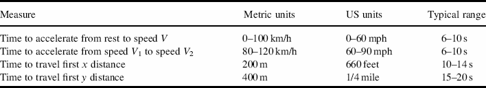
Owing to different driving conditions for different vehicle designs, the gear ratios may need adjustments to the initial design values. Practical test driving by experienced drivers can help to improve the performance of the vehicle by gear ratio refinements. A simple measure is the 0–100 km/h or 0–60 mph time which has become an accepted benchmark to describe the maximum acceleration performance of vehicles. Another important benchmark is the 80–120 km/h time as it relates to the ability of vehicle to overtake quickly. The time to cover 400 m or a quarter of mile time is another commonly used measure of a vehicle's performance. Table 4.3 summarizes some of these performance measures.
Example 4.3.9
For the vehicle in Example 4.3.3 the intermediate gear ratios using three different methods were designed in Examples 4.3.6–4.3.8. Compare the 80–120 km/h times for all three designs for both FWD and RWD vehicles.
Solution
The MATLAB program of Example 3.7.2 of Chapter 3 can be modified for this example. First, it must include a small loop to check which gears can produce the required speed of 120 km/h within the permitted engine speed range. Second, in the ‘while’ statement the engine speed at speed 120 km/h should replace the maximum engine speed. Required modifications are given in Figure 4.19. Using this program, the speed-time performance can be obtained for each of the three gear sets for both cases of FWD and RWD. The results are summarized in Table 4.4 in which N/P stands for ‘not possible’.
Table 4.4 80–120 km/h times (s) for Example 4.3.9

Figure 4.19 MATLAB program of Example 4.3.9

4.4 Gearbox Kinematics and Tooth Numbers
Once the gearbox ratios are available, the next step in gearbox design would be the determination of the number of gear teeth based on the speed or torque ratios rs and rT defined as:
(4.72) ![]()
(4.73) ![]()
in which the subscripts i and o stand for input and output respectively. Note that the gear ratio of a gearbox earlier denoted by n is exactly equal to rT. In an ideal gearbox with no power loss, the input and output powers are equal:
(4.74) ![]()
Therefore:
(4.75) ![]()
Thus in an ideal gearbox the speed and torque ratios are inverse of each other. For a couple of meshed gears, the torque ratio according to Figure 4.20 is:
Figure 4.20 Terminology used for two running gears

(4.76) ![]()
For a gear, the pitch diameter can be expressed in terms of the teeth number N:
(4.77) ![]()
in which m is the module of the gear; the same result could be obtained by expressing in terms of diameteral pitch. Hence:
For a gearbox with a number of meshed gears, the overall torque ratio is:
It should be noted that in a gearbox some of the ratios are unity since they belong to two gears on a compound shaft with a common angular speed. Equation (4.79) can be written in terms of the tooth numbers of the gears with substituting from Equation (4.78) for individual gear meshes.
In the process of selecting the tooth numbers in a gearbox, the tooth numbers of the pinion and the gear must be selected such that interference is prevented. The minimum number of teeth for pinion NP and the maximum number of teeth for the gear NG are given by following equations [3, 4]:
(4.80) ![]()
(4.81) ![]()
(4.82) ![]()
in which ψ, ϕn and ϕt are the helix angle, normal and tangential pressure angles of helical gears respectively (see Figure 4.21) and n is equal to the ratio of NG/NP. For spur gears ψ = 0 and the pressure angle ϕ must be used. Using these equations, the results obtained for spur and helical gears are provided in Tables 4.5 and 4.6.
Figure 4.21 Terminology of gears

For the example of spur gears, if a pressure angle of 20 degree and NP with 15 teeth is selected, then NG cannot have more than 45 teeth. Furthermore, for pressure angles of 20 and 25 degrees, the smallest numbers of teeth that can be selected regardless of the number of gear teeth are 18 and 12 respectively.
Table 4.5 NP and NG for spur gears.

Table 4.6 NP and NG for helical gears with normal pressure angle of 20.

4.4.1 Normal Gears
The normal design for gears used in manual transmissions nowadays is the constant mesh design (see Section 4.5). There are two types of gearbox designs according to the number of shafts. In the first design, only two input and output shafts are used as schematically shown in Figure 4.22 a. Each gear mesh denoted by 1, 2, etc. is a power transfer route in the transmission for each gear ratio and is selected through a shifting mechanism. In this type of gearbox, the input and output shafts are not in line, and hence it is suitable only for FWD transaxle applications. The second type uses three shafts, namely, the input shaft, layshaft and output shaft. Figure 4.22b schematically shows a five-speed gear set of this kind transferring power in gear 3. In this case a gear ratio involves two meshing pairs, one is the input pair denoted by ‘0’ and the other is any other of gear pairs 1, 2, etc. that is selected. This gear set is suitable for RWD applications as the input and output shafts are in line.
Figure 4.22 Layouts of manual gearboxes

Design of the tooth numbers of gears for the transaxle gear set involves the design of individual pairs but with a constraint for the centrelines of gear pairs:
In terms of tooth numbers:
(4.84) ![]()
With equal modules Equation (4.83) results in:
For the layshaft gear sets, Equation (4.85) also applies but in addition the gear ratio in each gear is a combination of two ratios:
(4.86) ![]()
in which (see Figure 4.23):
(4.87) ![]()
(4.88) ![]()

Therefore:
The following examples illustrate how to use the above equations to design the gear teeth numbers.
Example 4.4.1
Design gear numbers for a layshaft gearbox with a low gear ratio of 4. Gears are of helical type with a helix angle of 25° and normal pressure angle of 20°.
Solution
From Equations (4.89) and (4.85):
![]()
A table can be constructed for some possible values of two ratios ![]() and
and ![]() as shown in Table 4.7. If the first row is selected, we will have:
as shown in Table 4.7. If the first row is selected, we will have:
Table 4.7 Some possible alternative ratios for Example 4.4.1

![]()
Combining the two provides: ![]()
Since N, N1 and NP1 are all integer numbers, therefore N must also be a minimum integer of multipliers 2.25 and 4.2, or ![]()
![]()
Note that teeth number of 15 is permissible for this type of gear.
If the same procedure is used to determine the tooth numbers for the second row of the table, the result will be:
![]()
And the smallest gears are: ![]()
The results for the three alternatives are summarized in Table 4.8. As is clear, the results of the third case are smaller gears and make a smaller gearbox.
Table 4.8 Solutions to the alternative ratios for Example 4.4.1

The three options presented in the example were not the only choices one could have, for instance 3 and 4/3, 2.4 and 5/3, etc. are other options. In order to find the best solution for the problem, a table similar to Table 4.8 should be constructed and every possible choice must be investigated.
In general, the same procedure can be used to determine the tooth numbers for the other gear pairs. It should be noted, however, that in a layshaft gearbox for all engaged gears, the first ratio ![]() is the same. Thus the solutions for all gear ratios are dependent on each other and the solution must be obtained in an interrelated procedure. It should also be mentioned that the kinematic solution discussed in this section is a part of general solution in which the gears must be designed also for their structural integrity and durability in power transmission.
is the same. Thus the solutions for all gear ratios are dependent on each other and the solution must be obtained in an interrelated procedure. It should also be mentioned that the kinematic solution discussed in this section is a part of general solution in which the gears must be designed also for their structural integrity and durability in power transmission.
4.4.2 Epicyclic Gear Sets
The basic parts in automatic transmissions responsible for the gear ratios are planetary or epicyclic gear sets. Figure 4.24 shows a typical planetary gear set consisting of a sun gear S, a ring gear R and a number of planets P that have their rotation centres on a common carrier called the planet carrier C.
Figure 4.24 A typical planetary gear set (a) schematic, and (b) stick diagram

The ring gear has internal teeth and the other gears all have external teeth. The rotations of the planets are not of direct importance but the motions of their centres produce the rotation of the carrier which is important. The three angular speeds in a planetary set ωS, ωR and ωC can be related to one another via the rotations of planet gears. Defining the angular speed of a planet ωP (positive clockwise) gives:
in which R stands for the radius and is differentiated by the relevant subscripts. The carrier speed ωC can be written as:
(4.91) ![]()
where vp is the velocity of the planet centre:
Thus:
If all radii are expressed in terms of the gear modules, Equations (4.93) and 90 can be written in terms of tooth numbers:
(4.95) ![]()
Note that all angular speeds are taken as positive clockwise (see Figure 4.24).
Example 4.4.2
The sun, ring and planet gears in a planetary set have 30, 80 and 20 teeth respectively. The sun and ring are rotating at 100 and 50 rpm respectively. Determine the rotational speed of the carrier if:
(a) the sun and ring both are rotating clockwise;
(b) the sun is rotating clockwise but the ring is rotating counter-clockwise.
It should also be noted that an epicyclic gear set is a two degree-of-freedom device with two inputs and one output. In other words, if only one of the three angular speeds ωS, ωR and ωC were given, the system would be in an indeterminate state and the two other speeds could not be determined. When a planetary gear set is used as a vehicle gearbox, it must have one input and one output at a time. To this end, one degree of freedom must effectively be removed by fixing one of the three main rotating parts. For instance, if the ring gear is held stationary and the input is given to the sun gear, then the planet carrier will turn as the output of the system. For this configuration ωR = 0 and the overall gear ratio will be:
(4.96) ![]()
Two other useful input–output options are also possible and a summary of all three cases and their relevant gearbox ratios are presented in Table 4.9.
Table 4.9 Input–output alternatives of an epicyclic gear set.

The three gear ratios of Table 4.7 are related by following equation:
(4.97) ![]()
This also leads to:
(4.98) ![]()
Furthermore from the geometry of the set it is clear that:
(4.99) ![]()
This will result in alternative relations for the gear ratios:
(4.100) ![]()
(4.101) ![]()
(4.103) ![]()
An epicyclic gear set as seen has only limited number of gear ratios. For vehicle applications, therefore, multiple sets must be used in order to produce 4, 5 or more ratios (see Section 4.6.1).
Example 4.4.3
An epicyclic gear set is designed with a first ratio of 4. Determine the other ratios of the set.
Example 4.4.4
An epicyclic gear set is designed with a first ratio of 3.4. Determine the tooth numbers for all gears in the set.
Solution
The third ratio is:
![]()
From the third row of Table 4.7:
![]()
From Equation (4.92):
![]()
Thus:
![]()
Or:
![]()
The first choice could be:
![]()
Manual transmissions are the oldest kind of gearbox designs used in automobiles and were used for decades before automatic transmissions were introduced. Nevertheless, these transmissions are still popular due to their simplicity, low cost and high efficiency. The name ‘manual’ implies that the shifting from gear to gear must be performed manually by the driver. Although the manual transmissions are inherently the most efficient transmissions, their usage depends on the drivers' abilities and frequent manual operation is needed, for example, in urban traffic.
4.5.1 Construction and Operation
As Figure 4.25 illustrates, the transmission casing is directly bolted to the engine body through the bell housing which contains a space to accommodate the clutch system. The clutch assembly is bolted to the engine flywheel and the input shaft of the transmission receives power through the clutch plate. In fact, when the clutch is engaged, the input shaft of the transmission turns with the clutch at the same speed as the engine. Shifting is performed by means of a shifting mechanism when the transmission input is disconnected from the engine and a gear is selected by the shift lever.
Figure 4.25 Manual transmission assembly

The operation of the clutch is illustrated in Figure 4.26. The clutch is activated when the clutch pedal is depressed and the gear lever is pulled back, causing the release bearing to push the diaphragm spring. The seesaw effect of the spring pulls back the pressure plate and releases the clutch plate. The input shaft of transmission is directly fitted into the clutch plate through the splines and thus the two rotate with the same speed. In other words, although the clutch plate is placed inside the clutch system, it is effectively linked to the gearbox.
Figure 4.26 Details of the clutch mechanisms

There are two basic types of gear change: moving a gear to mesh the opposing gear, or moving a linking member to deliver torque to already meshing gears. The former type called the ‘sliding-mesh’ type is now an obsolete shifting method and its concept is shown in Figure 4.27 a. The second type that is used in all modern manual transmissions is the ‘constant-mesh’ design and its construction is schematically shown in Figure 4.27b. Both figures illustrate a layshaft type gearbox with in-line input and output shafts. The output shaft for both cases is splined. In the sliding-mesh type, the inside of the gear is also splined and can slide over the shaft. When the clutch is disconnected, the gear is moved to mesh with the opposing gear on the layshaft. Then, by releasing the clutch, the power will be transferred to the output shaft. In the constant mesh type the two opposing gears are in constant mesh (a pair for each gear ratio), but the gear on the output shaft has a hole in the centre and is not connected to the shaft and no torque is delivered between the two. The power transfer is done through a sliding collar with a spline in its core and dog teeth over its sides (see Figure 4.27b). The collar is always turning with the output shaft through the splines and when it is shifted to the side, its dog teeth fit into the matching teeth on the side of the gear and the three (shaft, collar and gear) connect to each other and power is transferred.
Figure 4.27 Sliding mesh and constant-mesh gear meshing methods

As the gear and output shaft in constant mesh design turn with different speeds prior to their engagement, there should be a means by which the speeds are synchronized. This device is called the ‘synchronizer’. Figure 4.28 shows the concept of using two matching conical surfaces that come into gradual contact as the collar slides towards the gear. When the two elements get close, the speeds gradually synchronize and the dog teeth subsequently engage.
Figure 4.28 Synchronizing concept

The gear selection and shifting mechanism is illustrated in Figure 4.29 in three views (front, top and left). For a typical five-speed transmission there are usually three forks that control the three collars and each collar is used to engage two gears when it slides to left or right. The forks are fixed on three rods that can move back and forth. The relevant rod is chosen by the left–right movement of the shift handle. Then the choice between the two gears related to a collar is made by the fore–aft movement of the gear lever or shift handle.
Figure 4.29 Shifting mechanism

4.5.2 Dry Clutches
A dry clutch is usually used with a manual gearbox for gear shifting. With reference to Figure 4.30, the engine torque is transmitted to the gearbox input shaft through the clutch plate locked between flywheel and pressure plate. The clutch assembly is bolted to the flywheel and as a result the pressure plate is always turning at engine speed. When the clutch is engaged, the spring force F is applied to the pressure plate forcing it against the clutch plate. Both sides of the clutch plate friction surfaces will receive the same force and produce half of the torque each.
Figure 4.30 Friction surfaces of a clutch plate

The basic mechanism for torque generation in the clutch plate is the existence of a normal load and slip that together produce friction forces at distances from the plate centre and result in a torque. The amount of torque of the clutch plate, therefore, depends on the normal force and slip values. During the clutch release these will vary with time and a transient torque transmission will result, starting from zero up to the torque capacity of the clutch. The transient behaviour is dealt with in Section 4.5.4 and in the next sections the nature of dry friction and the clutch torque capacity will be considered.
4.5.2.1 Dry Friction
According to the classic Coulomb friction model, when the surfaces of two bodies are in contact under the pressure of an external load W (see Figure 4.31), three cases may exist for a force F applied to a body in order to move it along the surface:
a. F is small and no relative motion is produced. In this case, the friction force Ff is simply:
(4.104) ![]()
b. F is large enough to bring the body to the point of slip. The friction force in this case is:
(4.105) ![]()
where ![]() is the static coefficient of friction.
is the static coefficient of friction.
c. The body skids (with a constant speed) over the surface. The friction force can be expressed as:
(4.106) ![]()
where ![]() is kinetic coefficient of friction and is normally smaller than
is kinetic coefficient of friction and is normally smaller than ![]() . For F larger than Ff the body will accelerate. In summary, by increasing the force F the friction force varies in the following range:
. For F larger than Ff the body will accelerate. In summary, by increasing the force F the friction force varies in the following range:
(4.107) ![]()
Even this simple model for dry friction Ff, has a non-linear nature when relative motion exists, because at speeds close to zero the value of coefficient of friction is close to the static value and at larger speeds it has its kinetic value. The coefficient of friction is influenced by parameters such as the types of contact surfaces, the relative velocity of the mating surfaces and the load. If the simple Coulomb friction model is considered, in the vicinity of zero speed, a transition from kinetic to static coefficient of friction must be included. For the clutch system before and during the engagement the flywheel rotates with engine speed ωe and the clutch plate with speed ωc as shown in Figure 4.32. The relative speed during the engagement period is:
Figure 4.32 Engine and clutch speeds during the clutch engagement

(4.108) ![]()
Therefore, the coefficient of friction for the clutch can be expressed as:
(4.109) ![]()
Simple models assume a linear transition from kinetic to static coefficient in the following form [5]:
(4.110) ![]()
in which α is a constant. Exponential transition is an alternative model in the form of [6]:
(4.111) ![]()
where β is a constant. A smoothing approach has also been used with Equation (4.112) in order that the same equation can be used for cases in which ![]() can switch from positive to negative values and vice versa [7]:
can switch from positive to negative values and vice versa [7]:
where σ is a constant value. Figure 4.33 illustrates the variation of coefficient of friction by using values β = 2, σ = 50, μS = 0.4 and μk = 0.25 for Equation (4.112).
Figure 4.33 Variation of friction coefficient with relative rotational speed

This model produces values of kinetic coefficient at most of the working points and the transition to the static friction occurs at very small slips. There are also friction models for the clutch that do not obey the Coulomb friction concept. The clutch torque Tc is taken as a factor of engine torque Te and slip speed [8]:
Figure 4.31 Two bodies with dry friction between them

(4.113) ![]()
The function f is dependent on the release-bearing displacement δB and slip speed, and is typically obtained through experiments.
4.5.2.2 Torque Capacity
The torque-transferring capacity of a dry clutch can be evaluated by a physical modelling approach. Figure 4.34 depicts a circular band of thickness dr on the friction surface of the clutch plate. Out of this strip an infinitesimal element of area dA is taken between two radial lines from the centre, making a small angle dθ. The enlarged view of this element is also shown in Figure 4.34. The application of an axial force F (Figure 4.30) creates a pressure distribution on the contact elements. Owing to circumferential symmetry with regard to angle θ, the pressure is identical at all points lying on a specific radius.
Figure 4.34 An infinitesimal element on the friction surface

Therefore, the pressure distribution is dependent on radius r only:
(4.114) ![]()
The normal force acting on the element dA is:
(4.115) ![]()
The resulting frictional force using the Coulomb friction model (see Section 4.5.2.1) is:
(4.116) ![]()
where μ is the coefficient of kinetic friction between the linings and the flywheel or pressure plate surfaces. To evaluate the torque transmission capacity of a clutch, the kinetic value of the coefficient is used since the clutch plate transmits the torque by slip. Different lining materials produce different friction coefficients ranging up to 0.5. A typical approximate value for a vehicle clutch application is 0.3 [9]. The contribution of clutch torque by the surface element is:
(4.117) ![]()
The total normal force acting on a clutch plate face can be found by integrating the infinitesimal normal forces over the whole friction surface, that is:
The total torque resulting from the friction elements on one side of clutch plate is the summation of infinitesimal torques dT. The whole torque transmission capacity of a clutch system is twice the capacity of one side, thus:
The results of Equations (4.118) and (4.119) depend on the pressure distribution p(r). Two different criteria exist for modelling the pressure variation on the clutch plate, namely uniform pressure and uniform wear.
Uniform Pressure Criterion
When two surfaces are in good uniform contact, it is reasonable to assume a uniform pressure distribution on all contact points. For the contact between the clutch plate and the flywheel or pressure plate surfaces, especially when the liners have flat surfaces, the contact can be regarded as uniform. The axial load applied by the clutch spring is also distributed evenly around the pressure plate. Therefore, a uniform pressure distribution can be assumed for the clutch plate friction surfaces. Defining this uniform pressure as pu, Equations (4.118) and 119 can then be integrated to find the total axial force Fup and transmitted torque Tup for the uniform pressure case:
For a certain outside diameter, the torque capacity will be maximum when the inner diameter is zero, i.e. an entire circular plate. It means that when a uniform pressure distribution exists, the torque transmitting capacity can be increased by extending the friction surface towards the inner areas. Since the clutch spring force is the main factor in torque capacity, it is useful to express the torque in terms of the spring force. Combining Equations (4.120) and (4.121) will lead to:
where:
or alternatively:
(4.124) ![]()
in which rav is the average radius of friction surface and kr being the ratio of inner to outer radii:
(4.125) ![]()
Uniform Wear Criterion
When an abrasive material is rubbed against a surface, the amount of particles separated from the material is proportional to the length of the path. In a clutch plate, materials located at distances further from the centre will experience more wear than those closer to the centre. The wear on the other hand depends on the normal load applied. In mathematical form, the amount of wear w can be taken to be proportional to both the pressure p and path length s:
(4.126) ![]()
k is the proportionality constant. The path length for the friction material located at radius r on the clutch plate in one revolution is ![]() and thus the wear of clutch friction material in one turn is:
and thus the wear of clutch friction material in one turn is:
The application of uniform wear criterion is to take w of Equation (4.127) to be a constant value w* at all radii to obtain:
(4.128) ![]()
which indicates the maximum pressure pm will occur at the minimum radius ri. The variation of pressure in radial direction is shown in Figure 4.35.
Figure 4.35 Radial pressure distribution

Eliminating w* will result in the pressure distribution for uniform wear case:
The existence of uniform wear means that regardless of the location, all parts of the material experience equal wear. This will result in a uniform and flat surface for the clutch friction material during its working life. Note that when a flat parallel friction surface exists, the uniform pressure assumption is also valid. Substituting Equation (4.129) into Equations (4.118) and (4.119) will provide the axial load and torque capacity for the uniform wear case:
According to Equation (4.130), when an axial spring force F is applied, for a certain outer diameter the maximum pressure pm will vary with the variation of the inner radius. Simple differentiation with respect to ri results that at the inner radius ![]() , pm will be minimum,
, pm will be minimum,
The torque capacity of the clutch for a certain value of outer diameter varies with the variation of the inner radius, as shown in Figure 4.36, and has a maximum value close to ri = 0.6 ro. The exact value can be found by differentiation of Equation (4.131) with respect to ri leading to ![]() .
.
Figure 4.36 Variation of clutch torque with radius ratio

Similar to the case of uniform pressure, the clutch torque can be written in terms of spring force:
Comparing to Equation (4.123), for this case:
(4.134) ![]()
4.5.2.3 Other Considerations
In practice, the surfaces of used clutch plates look fairly uniform and flat. Does this mean that the pressure distribution belongs to the uniform wear or uniform pressure? When the pressure is uniform over the surface, particles near the outer radius wear out faster than those near inner radius. As such, the pressure distribution will no longer remain uniform since the wear particles relieve the pressure when they disappear. Then, the pressure will be borne by the remaining particles, mostly at the inner radii. This results in higher pressures at the inner radii and lower presuures at the outer radii, which is the case of uniform wear. On the other hand, if the wear in the particles of clutch plate is uniform, the surface must remain flat and parallel, which provides the condition for uniform pressure distribution. Therefore, the pressure distribution can be either of two cases and can change from one to another.
One important point is that the clutch spring force is equal for both the uniform pressure and uniform wear case, no matter which case of pressure distribution exists. Therefore, when the spring load is selected, it must be suitable for both cases. With equal spring force, the torque capacity of the two cases can be compared. For instance, the ratio kT of torques can be obtained from Equations (4.121) and (4.131):
(4.135) ![]()
It is a simple task to show that the ratio of torque capacities at uniform pressure and uniform wear can be expressed in terms only of radius ratio kr:
This relation simply shows that at two extremes for kr, namely kr = 0 and kr = 1, the torque ratios are ![]() and 1 respectively. The variation of torque ratio for whole range of variation of radius ratio is illustrated in Figure 4.37, and shows that for equal spring loads the torque capacity at uniform pressure case is always greater than that of uniform wear. It is also useful to see the differences in the practical range of kr between 0.5 and 0.8.
and 1 respectively. The variation of torque ratio for whole range of variation of radius ratio is illustrated in Figure 4.37, and shows that for equal spring loads the torque capacity at uniform pressure case is always greater than that of uniform wear. It is also useful to see the differences in the practical range of kr between 0.5 and 0.8.
(4.137) ![]()
This shows a difference of somewhere between 0.4% and 3.7% for the torque capacities in the two cases of uniform pressure and uniform wear. Owing to this small difference, designing for either case will lead to similar results. Leaving a small margin for uncertainties in the value of coefficient of friction, it is reasonable to design using the uniform wear criterion.
Figure 4.37 Torque ratio kT versus radius ratio kr (Equation (4.136))

The torque capacity discussed so far has been the ability of clutch to transfer torque at the time of clutch engagement. When the clutch is locked up, the coefficient of static friction ![]() must be applied. For the locked-up clutch, therefore, the torque capacity is considerably higher than when it slips.
must be applied. For the locked-up clutch, therefore, the torque capacity is considerably higher than when it slips.
Example 4.5.1
A clutch is designed for a torque capacity of 200 Nm. The coefficient of friction is 0.4 and the outer clutch plate diameter must be a maximum of 200 mm:
(a) Calculate the inner radius for keeping the maximum pressure as small as possible.
(b) Determine the maximum pressure.
(c) Evaluate the spring force.
(d) Find the maximum torque capacity of the clutch.
Solution
(a) In order to keep the value of pm a minimum, the inner diameter must be taken to be half of the outer diameter: ![]()
(b) Maximum pressure can be calculated using Equation (4.131):
![]()
(c) The spring force can be evaluated using Equation (4.132): ![]()
(d) The maximum torque capacity will occur at uniform pressure case. From Equation (4.122) and using the spring force:
![]()
and torque capacity from Equation (4.123) is: ![]()
Lining Grooves
The grooves on the clutch linings help it cool down and also act as channels for removed particles to guide them out and leave a clean friction surface. The areas the grooves occupy, however, reduce the total friction area of the clutch linings. The rivet holes on the linings have also the same effect. A question may arise as to what extent this area reduction can influence the torque capacity of a clutch system. In order to answer this question, a simple model shown in Figure 4.38 is considered. For the sake of simplicity, the grooves are taken in pure radial directions which are different from those in practice which often have angled directions.
Figure 4.38 Grooves on the facing of a clutch plate

Assuming n grooves on the plate, the Equations (4.118) and (4.119) will become:
(4.138) ![]()
(4.139) ![]()
The parameters of the grooved surface will be denoted by a prime symbol and those of full friction surface with no prime. For the case of uniform pressure, assuming an identical clutch spring for the two models, results in:
(4.140) ![]()
Comparing with Equation (4.120):
which simply shows the pressure is higher since the same force is applied on a smaller surface. Evaluating the torque capacity results in:
(4.142) ![]()
Substituting from Equation (4.141) gives:
(4.143) ![]()
Therefore no change occurs to the torque capacity when grooves are included on the surface and the only effect is the pressure increase due to the surface reduction. It is a simple task to show that for the uniform wear case too, a similar result will exist.
Energy Loss
The energy loss due to friction in a clutch is the work done by friction forces. The infinitesimal work dW of the friction forces can be written as:
(4.144) ![]()
where:
(4.145) ![]()
and ![]() is the slip speed of clutch mating surfaces. Thus:
is the slip speed of clutch mating surfaces. Thus:
(4.146) ![]()
and,
(4.147) ![]()
The power loss due to friction is:
(4.148) ![]()
The energy and power losses can be calculated if instantaneous torque and speed of clutch are available.
4.5.3 Diaphragm Springs
Diaphragm springs are used in dry clutches to exert necessary force for the generation of friction torque. These springs are of conical shell form with a number of slots cut out in the upper part as schematically shown in Figure 4.39. Different circular or square holes are made at the bottom parts of the slots (not shown in Figure 4.39) to hold pivots or retaining bolts. The tips of so-called fingers come into contact with the release (or throw-out) bearing when clutch pedal is depressed (see Figure 4.40). At the engaged stage the release bearing is held away from the diaphragm spring's fingers. The diaphragm spring can be regarded as two separate springs joined together. The lower part of spring of Figure 4.39 is a Belleville spring and the upper part consists of several flat springs (fingers). The clamping force of the clutch is generated only by the Belleville part of the diaphragm spring.
Figure 4.39 A simple form of diaphragm spring

4.5.3.1 Function
The bottom part (outer rim) of the spring is in contact with the pressure plate. When the clutch is depressed, the release bearing pushes the fingers and the spring is pulled back (like a seesaw) and moves the pressure plate away from the clutch plate (see Figure 4.40).
Figure 4.40 Details of a clutch system

Three forces are important in the clutch system: the pedal force; the bearing force; and the spring force. The pedal force FP applied by the driver's foot is amplified by the leverage and a force FL is generated and transferred to the clutch lever input (see Figure 4.40). Once again this force is amplified and the bearing force FB results. The bearing force is transmitted to the spring and causes the spring force on the clutch plate to decrease. The bearing force is related to the pedal force based on the geometry shown in Figure 4.40:
4.5.3.2 Spring Forces
Three groups of forces acting on the clutch spring are schematically illustrated in Figure 4.41. These include those exerted by the release bearing on the finger tips, those exerted by the retainers at the spring holes (support forces), and the reaction forces from the pressure plate.
Figure 4.41 Forces acting on the diaphragm spring

The forces acting on the pressure plate are reaction forces from the spring and the clutch plate that balance each other. Hence, the force that compresses the clutch plate between the pressure plate and the flywheel is in fact equal in magnitude to the reaction force on the spring and is called the ‘clamp load’. In the engaged state with no bearing force, the diaphragm spring pivots over its slot rings and its outer rim forces the pressure plate tightly against the clutch plate with force FS due to a preload. In fact, before the clutch assembly is bolted to the flywheel, as illustrated in Figure 4.42a, the diaphragm spring is free and the cover will remain at a distance δ0 from the flywheel surface. Bolting the cover to the flywheel forces the spring into a pre-loaded condition shown in Figure 4.42b.
Figure 4.42 The clamp force resulting from preload

The application of the bearing force will cause the bearing to move towards the flywheel by bending the spring fingers. The change of the bearing force FB with its displacement δB has a non-linear characteristic as shown in Figure 4.43 for a typical small passenger vehicle. Since the bearing load releases the clutch from engagement, this force is commonly called the ‘release load’.
Figure 4.43 Typical bearing force (release load) variation

The force exerted on the clutch plate by the pressure plate, i.e. the spring force FS, results from the tensioning the spring between the outer rim and the retainers. In fact, the spring fingers are not involved in the generation of this force. In order to obtain a better understanding of how the spring force is generated, consider the clutch system of Figure 4.44 in which the cover is rigidly fastened to a flat surface and a disk is put under the pressure plate instead of the clutch plate. In the beginning, the displacement δ relative to the reference line is zero when no force is applied. The application of force will cause a displacement δ.
Figure 4.44 Definition of spring force

The variation of the spring load FS with the spring travel δS is typically of the form shown in Figure 4.45. It increases up to a peak with increase in the displacement, then starts to decline to a minimum and afterwards increases exponentially. With reference to Figure 4.42 when a clutch plate is placed between the pressure plate and the flywheel, the pressure plate will undergo an initial displacement δS* = δ2-δ1, due to the contraction of the clutch plate cushion springs. On the clamp load diagram (Figure 4.45), the load at the displacement δS* describes this situation. For a new clutch plate, the thickness of linings is a maximum and the preload point on the diagram, called the ‘set load’ point, will be at the far right. By the time the linings wear out, the initial displacement gradually reduces and brings the working point to the left, up to the points at which the plate rivets come into contact with the surface of flywheel (or pressure plate). This is indicated by ‘wear-in load’ in Figure 4.45. This range from the minimum to the maximum displacement, which is typically of the order of 2 mm, is called the ‘wear-in area’. The shaded segment of Figure 4.45, therefore, should not be used.
Figure 4.45 Typical force-deflection curve of diaphragm spring

In order to release the clutch plate, the pressure plate must be moved away from the flywheel which means the spring's displacement must increase relative to its initial value of δS*. In Figure 4.45, this means moving further to the right. To move the pressure plate away from the flywheel and release the clutch plate, no force can be applied from the inner part and hence, the releasing force is applied to the bearing in the opposite direction! When the bearing force acts on the diaphragm spring's fingers during the disengagement stage, due to the pivoting action, the spring contact force, i.e. the clamp load FC, is reduced.
Assuming a symmetrical loading on the spring, Figure 4.41 is simplified by taking only a segment shown in Figure 4.46 in which the shaded part is the spring body and the unshaded part represents the finger. To make it simple, it is assumed this segment supports the full load of the diaphragm spring as a whole. This segment is in static equilibrium under the action of several forces. The segment is supported at the pivot S by unknown forces. The clamp force FC and the friction force FX are acting at the pressure plate's contact point C. The bearing force FB acts at the finger tip and at the cuttings (shaded areas) there are forces (not shown) that are all moved to the pivot point S together with their resulting moments MS about S.
Figure 4.46 Free body diagram of a diaphragm spring's segment

The moment balance about point S is (positive clockwise):
FX is the friction force at point C, thus:
(4.151) ![]()
Therefore, Equation (4.150) can be rewritten as:
(4.152) ![]()
The term ![]() is small compared to unity (some 2–5%) and it is reasonable to ignore it. On the other hand, the moment MS in fact is the spring's resistance to the applied load and increases when the spring deflection δS increases. In other words, it is equal to the moment of the spring's elastic force about the point S:
is small compared to unity (some 2–5%) and it is reasonable to ignore it. On the other hand, the moment MS in fact is the spring's resistance to the applied load and increases when the spring deflection δS increases. In other words, it is equal to the moment of the spring's elastic force about the point S:
(4.153) ![]()
Thus, the clamp force equation in general can be written as:
in which ks will be called the ‘seesaw gain’:
(4.155) ![]()
and δB is the releasing bearing displacement, δP is the pressure plate lift-off displacement and δS is the total spring deflection:
(4.156) ![]()
Referring to Figure 4.42, the initial deflection ![]() of the spring is:
of the spring is:
Typical variations of FB versus ![]() and FS versus
and FS versus ![]() are shown in Figures 4.43 and 4.45. In order to be able to use Equation (4.154), the two displacements δB and δP must be related and belong to a unique working condition of the spring. Theoretically, this relationship can be obtained by the application of the virtual work principle to the spring of Figure 4.46. If a virtual displacement ΔB is applied at the point of action of FB, the other forces will also experience virtual displacements Δ for FX, ΔP for FC and Δθ for MS as shown in Figure 4.47.
are shown in Figures 4.43 and 4.45. In order to be able to use Equation (4.154), the two displacements δB and δP must be related and belong to a unique working condition of the spring. Theoretically, this relationship can be obtained by the application of the virtual work principle to the spring of Figure 4.46. If a virtual displacement ΔB is applied at the point of action of FB, the other forces will also experience virtual displacements Δ for FX, ΔP for FC and Δθ for MS as shown in Figure 4.47.
Figure 4.47 Virtual displacements

Since the whole system is in equilibrium, the net virtual work done by all forces and moments should be nil. In mathematical form:
(4.158) ![]()
According to Figure 4.47 and assuming small Δθ, the virtual displacements can readily be related:
(4.159) ![]()
(4.160) ![]()
Therefore:
Substituting for the parenthesis from Equation (4.150) gives:
(4.162) ![]()
With a small deflection approximation, the total displacements δB and δP can be related by:
Owing to the non-linear behaviour of the spring, however, the actual relationship is not linear. A typical dependency of the pressure plate's displacement δP on the bearing displacement δB for a passenger car clutch is shown in Figure 4.48. A linear approximation is also considered together with a dead zone in which the pressure plate is insensitive to the bearing displacement.
Figure 4.48 Relationship between the pressure plate and bearing displacements

With a linear relation of Equation (4.164), the clamp force of Equation (4.154) can be rewritten as:
On the other hand, the clamp load is simultaneously acting on the clutch plate causing its cushion springs to deflect (see Figure 4.42). Thus, the clamp load can also be related to the cushion springs deflection characteristics. During the clutch disengagement two phases will exist; the first phase is the clamp load reduction and second phase is the pressure plate and clutch plate separation. In the first phase, the clamp load reduces from its initial value of FS* to nil, and causes the cushion spring inside the pressure plate to expand to its initial deflection ![]() (see Figure 4.42):
(see Figure 4.42):
(4.165) ![]()
Using Equation (4.157) one finds:
Therefore, the total displacement of pressure plate in the first phase, just before disengagement, is δC*. At the end of first phase the clamp load disappears. This instant identifies the start of the second phase at which the clutch plate and pressure plate begin to separate (pressure plate lift-off). A typical variation of the clamp load during phase 1 according to Equation 4.164 can be seen in Figure 4.49.
Figure 4.49 Variation of the clamp load with pressure plate displacement

4.5.3.3 MG Formula
Equation (4.164) is useful when the variations of the spring and bearing forces with relevant displacements are available. Such information can be obtained from clutch tests. The test equipment applies independent forces to the finger tips and pressure plate in order to measure the bearing and spring forces. A clutch under test is shown in Figure 4.50 and a typical test result is given in Figure 4.51. The graphs illustrate the hysteresis behaviour of the spring due to the inherent internal friction.
Figure 4.50 Clutch test equipment

Figure 4.51 Typical test results for spring force

As the spring force results from the Belleville part of the spring, the mathematical equation for the force-displacement curve of such springs has usually been used to express the behaviour of a diaphragm spring. Research work was carried out at the Department of Automotive Engineering, IUST, in which the test results for several clutch springs were used in order to develop a more accurate relationship between the spring force and its displacement. The final result was found to be applicable to all tested springs belonging to C and D segment automobiles as well as light truck clutches. The spring force-displacement equation which will be called the MG formula (stands for Mashadi-Ghyasvand), that uses the basic Belleville equation with several modifications, is of the following form:
in which δS is the spring deflection (mm) and FS is calculated in kgf. The other parameters are:
(4.168) ![]()
(4.169) ![]()
(4.170) ![]()
(4.171) ![]()
(4.172) ![]()
(4.173) ![]()
The definition of geometrical parameters can be found in Figure 4.52. E and ν in Equation (4.167) are modulus of elasticity (MPa) and Poisson's ratio of the spring material respectively. A comparison is made between the results of the MG formula with the experimental measurements in Figure 4.53. The central part of the figure which describes the working area of the spring shows good agreement.
Figure 4.52 The geometry of diaphragm spring

Figure 4.53 Comparison of test data with results of spring MG formula

A similar equation for the release load (bearing force FB) versus the bearing displacement δB is also obtained in the following form:
(4.174) ![]()
in which:
(4.175) ![]()
(4.176) ![]()
Example 4.5.2
The information for a passenger car clutch is given in Table 4.10.
(a) Plot the FS -δS and FB-δB curves using the MG formula.
(b) Calculate the seesaw gain ks.
(c) Plot the variation of clamp force inside the first plot of FS-δS.
(d) Calculate the initial deflection ![]() .
.
Table 4.10 Clutch data for Example 4.5.2
| Parameter | Value | Unit |
| Inner diameter Di | 62 | mm |
| Outer diameter Do | 206 | mm |
| Belleville inner diameter Db | 171.3 | mm |
| Spring thickness t | 2.3 | mm |
| Belleville height h | 3.47 | mm |
| Set point deflection |
3.5 | mm |
| Modulus of elasticity | 207 | MPa |
| Poisson's ratio | 0.3 | – |
Solution
(a) With a simple MATLAB program the required curves can be plotted. The results are given in Figure 4.54.
(b) Referring to Figure 4.52:
![]()
(c) Using Equation (4.164), the variation of clamp load is obtained and then plotted against the variation of pressure plate displacement. Figure 4.55 shows the result. Note that in Figure 4.49a similar result was plotted against the bearing displacement. It should also be noted that the graphs are invalid after the clamp load vanishes (shaded area).
(d) According to Equation (4.166):
![]()
Therefore:
![]()
Figure 4.54 Spring and bearings forces of Example 4.5.2 (a)

Figure 4.55 Clamp load versus pressure plate displacement

4.5.4 Clutch Engagement Dynamics
In a vehicle equipped with a manual gearbox, for a gearshift it is necessary to press and hold the clutch pedal in order to disconnect the engine from the driveline. When the gear is shifted, then releasing the clutch will let the flywheel and gearbox input shaft gradually attain equal speeds. During this period, torque is generated between the sliding surfaces due to friction which is controlled by the normal force applied to the mating surfaces. The speed variations of the two mating surfaces are dependent on the dynamics of the process influenced by the values of the load and the inertia of input and output. Figure 4.56 depicts a typical speed variation during clutch release with the first gear engaged.
Figure 4.56 Engine and clutch speeds during clutch release

The clutch release is performed by gradually lifting the pedal which will increase the spring force on the surfaces. The resulting torque Tc is proportional to the applied force F (see Equations (4.122) or (4.133)):
K is the proportionality constant equal to ![]() or
or ![]() for the uniform pressure or uniform wear respectively. Let Te be the flywheel input torque, i.e. the torque received from the engine side, and TL the load torque on the clutch, i.e. from the driveline. Figure 4.57 depicts the free body diagram of the flywheel and clutch plate with torques Te and TL as input and load torques as well as Tc as the friction torque acting on contact surfaces. The inertia properties are described by Ie as the overall inertia of input shaft and all connecting parts, and Id as the overall inertia of the output shaft and all connecting parts.
for the uniform pressure or uniform wear respectively. Let Te be the flywheel input torque, i.e. the torque received from the engine side, and TL the load torque on the clutch, i.e. from the driveline. Figure 4.57 depicts the free body diagram of the flywheel and clutch plate with torques Te and TL as input and load torques as well as Tc as the friction torque acting on contact surfaces. The inertia properties are described by Ie as the overall inertia of input shaft and all connecting parts, and Id as the overall inertia of the output shaft and all connecting parts.
Figure 4.57 Free body diagrams of clutch mating plates

The driveline equivalent inertia Id referred to the clutch plate can be written as (see Figure 4.58):
Figure 4.58 Inertias in a vehicle driveline

(4.178) ![]()
in which Ic is the inertia of clutch shaft and all connected masses, Ig is the equivalent inertia of gearbox output shaft and differential input shaft, and Iw is the inertia of wheels and axles combined. ng and n are the gearbox and overall transmission gear ratios, m is the vehicle mass and rw is the wheel effective radius.
The dynamic equations for the two sides during the clutch engagement are (see Figure 4.57):
It should be noted that in these equations the elasticity of input and output shafts as well as the damping torques in the bearings have been ignored for the sake of simplicity; these will be dealt with in Chapter 6. The input and load torques are time-varying in general; the input torque variations depend on the throttle input, whereas the load torque is dependent on the vehicle's external loads.
The power flow in the clutch system is also important. A part of engine power Pe is transferred to the clutch (Pc) and some part is consumed by the rubbing friction surfaces (Pf). These are:
(4.181) ![]()
(4.183) ![]()
In order to determine the power relationships, let us begin with the difference ![]() :
:
(4.184) ![]()
This can be simplified by using Equations (4.179) and (4.182):
Thus the clutch power Pc is not the difference between the input power and friction power, since a part of input power is also used to change the kinetic energy of the flywheel. Note that the power flow is instantaneous, as is clear from the differentiation sign of Equation (4.185). Therefore, it is only in the steady-state condition that a power balance equation from input to the output can be written. In other conditions, the energy term is important. A misunderstanding is sometimes seen in the literature of taking the engine and clutch powers to be equal at times close to clutch lock-up. Equation (4.185) clearly shows that this assumption is far from being true, unless the engine speed is kept constant. Note that Pf will vanish as it approaches lock-up.
Clutch efficiency during engagement can be defined as:
where the input energy Ei, energy at lock-up EL and energy loss Eloss are:
(4.188) ![]()
(4.189) ![]()
where tL is the time when the speeds of flywheel and clutch plate become equal and the full engagement or clutch lock-up is achieved. After lock-up, Equations (4.179) and (4.180) can be combined to obtain:
(4.190) ![]()
Equation is the governing equation for engine dynamics after the clutch lock-up.
In order to evaluate TL, one should consider the external loads acting on the vehicle, details of which were discussed in Chapter 3. These comprise rolling resistance, aerodynamic, and grade forces. With the assumption of no wheel slip (see Section 3.10), the load torque can be written as:
(4.191) ![]()
The variation of the clutch force with time depends on two factors; one is the spring's force-displacement behaviour and the second is the way the clutch pedal is released. The former can be obtained from the characteristics of the diaphragm spring (Section 4.5.3) and the latter is an input to the model. Details of the dynamic behaviour of clutch engagement require information on the throttle inputs and clutch release regime and will be discussed in the following sections.
4.5.4.1 Uniform Clutch Release
Let us assume the clamp force of clutch varies linearly with the release bearing's displacement, then for a uniform release of clutch, the clutch force can be considered to increase linearly with time by a constant factor kF, i.e.,
Equation (4.192) is valid only for times when the force does not exceed its limiting value Fmax:
(4.193) ![]()
The output torque will also grow linearly with time by factor KkF (see Equation (4.177)):
(4.194) ![]()
The variations of the clutch force and torque for these linear assumptions can be illustrated in graphical form of Figure 4.59.
Figure 4.59 Clutch force and torque time variations (linear assumption)

Considering the fact that the maximum clutch torque is delivered at the maximum clutch force, for input torques smaller than the maximum torque, the time tT at which the friction torque becomes equal to the input torque will always be smaller than tr, the time of the maximum force. In other words, when the clutch starts to engage, the clutch torque reaches the input value before the clutch is completely released. The time tT depends on the value of input torque Ti:
(4.195) ![]()
The clutch force at the end of this phase is (see Figure 4.59):
(4.196) ![]()
At this time, the clutch torque is equal to the input torque, but the clutch output speed is still below the input speed. This means the full power is not delivered to the output since the same input torque is transmitted to the output but at a lower speed. Further release of the clutch will increase the spring force and in turn also increase the clutch torque up to its maximum limit. With known characteristics for Tc and TL, Equation (4.180) can be integrated to find the clutch rotational speed before lock-up:
The vehicle acceleration and speed during this period are:
(4.198) ![]()
(4.199) ![]()
The distance travelled can also be found from:
(4.200) ![]()
Also from Equation (4.179):
The integral on the left side depends on the throttle input and engine speed and in general is difficult to obtain. After lock-up the speed of the engine and clutch can be found by the integration of Equation:
(4.202) ![]()
where tL is the lock-up time.
There is a subtle issue regarding the rolling resistance part of the load torque in the equations of this section. In fact, on a level road, no load will act on the vehicle as long as a motive force is not present. Thus for those instants with no clutch torque, no load torque should be considered. Also as long as the clutch torque is less than the rolling resistance torque, the net motive torque on the clutch plate must be zero. In other words, the rolling resistance torque alone cannot produce a negative acceleration.
Constant Engine Torque
If a constant engine torque T* is assumed to be delivered during the clutch engagement, then the integral of Equation (4.201) and engine speed ![]() can readily be obtained from Equations 4.179 and 4.194:
can readily be obtained from Equations 4.179 and 4.194:
The time tL at which the two speeds become identical (lock-up time) can be found by equating Equations (4.201) and (4.203):
(4.205) ![]()
where:
(4.206) ![]()
(4.207) ![]()
(4.208) ![]()
The angles the engine and clutch plate revolve (in radians) are found by integrating Equations (4.204) and (4.197):
(4.209) ![]()
(4.210) ![]()
The speed of flywheel after lock-up can be found from:
(4.211) ![]()
The clutch efficiency during engagement is determined by using Equations (4.187) and 189 then substituting in Equation (4.186). The input and loss energies are:
Example 4.5.3
Consider a 1 second time for a uniform release of clutch pedal and assume that the engine torque during this period is kept constant. The vehicle is at a standstill and a gradual start-up on a level road is required.
(a) Calculate the clutch lock-up time.
(b) Plot the variation of engine and clutch speeds up to the lock-up point.
(c) Plot the variations of engine and clutch torques.
(d) Plot the variations of components of powers.
(e) Determine the clutch efficiency during the engagement.
(f) Discuss the results.
Data are given in Table 4.11.
Table 4.11 Data for Example 4.5.3
| Parameter | Value | Unit |
| Input inertia Ie | 0.25 | kgm2 |
| Clutch inertia Ic | 0.05 | kgm2 |
| Gearbox output inertia Ig | 0.1 | kgm2 |
| Wheels and axles inertia Iw | 2.0 | kgm2 |
| Vehicle mass | 1000 | kg |
| Wheel radius | 30 | cm |
| Gearbox ratio | 3.5 | – |
| Final drive ratio | 4 | – |
| Rolling resistance coefficient | 0.02 | – |
| Engine input torque (constant) | 60 | Nm |
| Maximum engine torque | 110 | Nm |
| Engine initial speed | 1000 | rpm |
Solution
K and kF are not given. We assume the clutch is designed for the maximum engine torque which leads to: ![]()
A simple MATLAB program can be written to calculate the variables. Figure 4.60 provides a sample program for this purpose. The answer to (a) using this program is: ![]() .
.


The results of (b) and (c) are plotted in Figure 4.61. The results of (d) are plotted in Figure 4.62.
Figure 4.61 Answers to (b) and (c) of Example 4.5.3

Figure 4.62 Answers to (d) of Example 4.5.3

The result of (e), the efficiency of clutch during engagement is 44.7%.
(f) The speed of the engine increases while the clutch torque is small, and then decreases with the increase of the clutch torque. The clutch speed, on the other hand, grows steadily to reach the engine speed. The clutch torque increases linearly with time, but as is clear from the lower subplot of Figure 4.62, its maximum exceeds the maximum torque of engine (110 Nm). The reason is that the release time of 1 second for the uniform increase of clutch force was not sufficient for the speeds to become equal. At 1 second the torque attains the 110 Nm limit and should not increase further. Thus, the results after 1 second are not valid.
The power variations, on the other hand, show that the friction power grows steadily up to around 0.65 sec and declines afterwards with decreasing slip speed. The surface under the net instantaneous power depicted in the lower subplot indicates the net energy transmitted to the system by the engine. Therefore, the remaining engine power is lost to friction or external load on the vehicle. The power lost to friction (Pf) is large compared to the power consumed by the external load (Pl).
Note that the clutch power slightly after 0.9 second is larger than the input power from the engine. This is because the clutch plate is receiving not only a part of engine power, but also a considerable amount of kinetic energy from the flywheel (this is why the engine speed decreases). In Equation (4.185) with a negative engine acceleration and decreasing friction power, the clutch plate receives additional power and its power value is higher than the engine power.
Constraint on Torque
We earlier noticed that the torque will grow higher than its maximum limit unless a constraint is imposed on it:
(4.214) ![]()
For the constant clutch torque region, the engine and clutch speed variations are:
(4.215) ![]()
(4.216) ![]()
Vehicle acceleration, velocity and travelled distance during this period are:
(4.217) ![]()
(4.218) ![]()
(4.219) ![]()
The new lock-up time ![]() at which the two speeds become identical is:
at which the two speeds become identical is:
(4.220) ![]()
Example 4.5.4
Repeat the previous example with a constraint imposed on the clutch torque. In addition to (a) plot of speeds; (b) plot of torques; also (c) plot the variations of vehicle acceleration, speed and travelled distance with time.
Solution
Small changes to the previous program can include the torque constraint. A sample program for these changes is given in Figure 4.63. The results obtained with this program are depicted in Figures 4.64 and 4.65.
Figure 4.63 Changed parts of program for Example 4.5.4

Figure 4.64 Answers to (a) and (b) of Example 4.5.4

Figure 4.65 Answers to (c) of Example 4.5.4

The lock-up time ![]() becomes only slightly longer than tL:
becomes only slightly longer than tL: ![]()
The overall trends of parameters are similar to previous results. Although the torque limitation is applied, no significant changes occur due to the very short period of time involved.
Throttle Inputs
In practice, the clutch engagement is performed by controlling the throttle at the same time as the clutch pedal is released. In this way the engine torque is controlled in accordance with power requirements which comprise the power generated by the clutch torque on the output shaft and the dissipated power due to friction.
With a uniform clutch release assumption, the clutch torque variations will be similar to those described before. For different throttle inputs, different scenarios can be considered:
- Sudden throttle: In this case, a throttle value of θ0 is applied instantly as the releasing is underway.
- Constant throttle: In this case, a throttle value of θ0 is assumed to be applied before the releasing is performed. Therefore, prior to the release, the engine speed is higher than sudden throttle case.
- Variable throttle: In this case, the throttle is assumed to vary in an exponential form according to the load on the vehicle and final throttle value
 is chosen by the operator. The relation is:
(4.221) ![]()
(4.222) ![]()
in which ![]() is the initial throttle input and coefficients a, c and d are three constants.
is the initial throttle input and coefficients a, c and d are three constants.
Owing to the complexity of engine behaviour following throttle inputs, no closed form solution is available for this case. A computer program, therefore, is needed for the solution of governing differential equations. Similar problems were solved in Chapter 3 and the same program structure can also be used in the current case.
Example 4.5.5
For the vehicle in Example 4.5.3, consider a sudden throttle input of 35% at the start-up and repeat the calculations. The MT engine formula coefficients and full throttle engine data are available in Tables 3.1 and 3.2 of Chapter 3.
Additional information is provided in Table 4.12.
Table 4.12 Additional data for Example 4.5.5
| Parameter | Value | Unit |
| Coefficient of dynamic friction | 0.20 | |
| Initial engine speed | 1000 | rpm |
| Average clutch radius | 15 | cm |
Solution
A main MATLAB program is generated together with two MATLAB functions to solve the differential equations. The structure of the programs is similar to previous examples and comments inside the program listings given in Figures 4.66 and 4.67 are self-explanatory.
Figure 4.66 Main MATLAB program for Example 4.5.5


Figure 4.67 MATLAB functions for Example 4.5.5

Results obtained from these programs are illustrated in Figures 4.68–4.70. Solid lines in general belong to engine outputs and dashed lines are for clutch outputs. The outputs for the rotational speeds and torques of clutch and engine depicted in Figure 4.68 show quite similar results to those of previous examples with constant torque. The reason is that the torque has a very small variation and the amplitude is close to that of Example 4.5.4.
Figure 4.68 Engine and clutch speeds and torques of Example 4.5.5

Figure 4.69 Power elements (see Figure 4.62) of Example 4.5.5

Figure 4.70 Engine throttle, engine and clutch turns of Example 4.5.5

The lock-up time in this case is 1.091 s, again very close to the previous result. Power elements depicted in Figure 4.69 are also quite similar to those in Example 4.5.4. In this case, the number of turns of flywheel and clutch plate are also calculated and shown in Figure 4.70.
The clutch efficiency during the engagement in this case can be found by including the following additional integrations in the function:
delomeg=abs(×(1)−×(2));f(5)=Te*×(1);f(6)=Tc*delomeg;
and the following statements in the main program:
Ei=×(i,5)+0.5*Ie*(w0*pi/30)^2;Eloss=×(i,6);etac=(Ei−Eloss)*100/Ei;
The result is 45.5%.
Note that the similarities between the answers of Example 4.5.4 and the current example are due to the identical vehicle parameters and the choice of 35% throttle input that produced similar torque inputs. The maximum torque of the MT engine model is 113 Nm, whereas in Example 4.5.4 it was 110. Therefore only small differences exist between the results of the two cases. This example was designed to show that the assumption of a constant engine torque is reasonable.
Example 4.5.6
Repeat Example 4.5.5 for an exponential throttle input with values of a, c and d equal to 3, 3 and 2 respectively. The vehicle in this case is initially at rest on an uphill road with a slope angle of 10 degrees. For this case consider a pedal release time of 1.5 sec and a final throttle value of 50%.
Solution
With small modifications to the programs of Example 4.5.5 (not provided), the results shown in Figures 4.71–4.73 are obtained. Since the vehicle is facong uphill, a backward motion occurs as shown by negative clutch speed of Figure 4.71. The 50% throttle is enough to prevent engine speed falling below 1000 rpm at the time of lock-up. The power curves of Figure 4.72 indicate that the instantaneous power becomes negative at times.
Figure 4.71 Engine and clutch speeds and torques of Example 4.5.6

Figure 4.72 Power elements (see Figure 4.62) of Example 4.5.6

Figure 4.73 Engine throttle, engine and clutch turns of Example 4.5.6

4.5.4.2 Pedal Release
The most realistic case for clutch dynamics would be to consider the clutch pedal travel instead of the clutch force variation during the engagement. To this end, the relationship between the pedal travel and the release bearing travel can be obtained similar to Equation (4.149) (see Figure 4.40). Assuming rigid arms, the displacement δB of release bearing is related to pedal travel xP by:
(4.223) ![]()
Making use of Equation (4.163), one will find the relationship between the pressure plate displacement δP and the pedal travel xP:
Now according to Equation (4.164), the clamp force FC can be determined from the pedal travel xP. Thus, the clutch dynamics will depend on the time history of pedal travel xP(t) during clutch release. In order to analyze the clutch dynamics by pedal travel, the following examples are presented.
Example 4.5.7
The measured lever arms of a clutch system in a vehicle are given in Table 4.13.
Table 4.13 Clutch system information for Example 4.5.7

(a) Calculate the overall gain from the pedal travel to pressure plate displacement.
(b) For a maximum displacement of 13 cm for the clutch pedal, determine the pressure plate displacement.
Solution
The answer to (a) can be found from Equations 4.163, 4.223 and (4.224):
![]()
![]()
![]()
The answer to (b) simply is:
![]()
Example 4.5.8
For the clutch of Example 4.5.7, the information on the MG formula is provided in Table 4.14. If a linear pedal release in 2 seconds is considered:
(a) Determine displacement ![]() that takes place before the release bearing comes into contact with the spring fingers.
that takes place before the release bearing comes into contact with the spring fingers.
(b) Plot the time variations of the clamp load and displacements.
Table 4.14 Clutch data for Example 4.5.8
| Parameter | Value | Unit |
| Inner diameter Di | 46 | mm |
| Outer diameter Do | 164 | mm |
| Bellville inner diameter Db | 134.5 | mm |
| Spring thickness t | 2 | mm |
| Bellville height h | 2.75 | mm |
| Set point deflection |
3 | mm |
| Modulus of elasticity | 207 | MPa |
| Poisson's ratio | 0.3 | – |
Solution
A linear pedal release in 2 seconds means that the maximum displacement of 13 cm has travelled linearly:
Figure 4.74 MATLAB program for Example 4.5.8

![]()
Therefore: ![]()
For the pressure plate displacement, however, we need to find out when the bearing comes into contact with the fingers. This happens just before the clamp force starts to build up from zero. From Equation (4.164) the transition point is:
![]()
which is a nonlinear function and must be solved numerically (or by trial and error) to obtain ![]() , that is the total displacement of the bearing from start of contact between the clutch plate and pressure plate to completion of the engagement. Hence, the rest of bearing travel
, that is the total displacement of the bearing from start of contact between the clutch plate and pressure plate to completion of the engagement. Hence, the rest of bearing travel ![]() is to bring the pressure plate into contact with the clutch plate, i.e.,
is to bring the pressure plate into contact with the clutch plate, i.e.,
![]()
In the time domain it is:
![]()
The pressure plate displacement is zero up to this time and after that it is:
![]()
When the time history of the displacements is known, the clamp force can be obtained from Equation (4.164).
A MATLAB program is useful for solving the equations given above. A sample program is provided in Figure 4.74. The function used to determine ![]() is shown in Figure 4.75.
is shown in Figure 4.75.
Figure 4.75 MATLAB function for Example 4.5.8

Figure 4.76 Time histories of clutch displacements

Figure 4.77 Time histories of clutch forces

Parameters ![]() ,
, ![]() and
and ![]() calculated by the program are:
calculated by the program are:
![]()
Therefore, when the pedal is fully depressed, the bearing displacement is 5.456 mm. Releasing the pedal up to 1.087 seconds, only brings the pressure plate in contact with the clutch plate and clutch engagement starts here. So far the bearing has displaced 3 mm whereas the pressure plate has displaced 0.943 mm (Figure 4.76). In the remaining time of 0.9 seconds the engagement takes place and the clamp force increases from zero to its maximum of 406 kgf (Figure 4.77) that is equal to spring force at its set point.
Example 4.5.9
Use the information of Examples 4.5.3, 4.5.7 and 4.5.8 and simulate the clutch dynamics by releasing the clutch pedal when a constant engine torque is maintained.
Solution
A suitable program for this example is a combination of programs written for Examples 4.5.5 and 4.5.8. Modifications are needed since the program of Example 4.5.5 was for throttle input whereas for the current example a constant torque is assumed.
Preparing this program is left to the reader and only the results are given here. The time variations of the rotational speeds as well as torques of engine and clutch plate are illustrated in Figure 4.78. Since the engagement phase starts after around 1.1 sec, and the torque input is present from the start, the engine speed increases close to 4000 rpm until the release period begins and the clutch torque opposes the input torque. The clutch torque is determined from the clamp load and the coefficient of friction, and as a result it grows to large values but the torque limit is imposed at 110 Nm (max. of engine torque). The plot of power items given in Figure 4.79 shows a similar trend in the engagement phase, but with larger values of friction power that produce negative power flows during this stage.
The efficiency of the clutch engagement is found to be 40.1%.
Figure 4.78 Turning speeds and torques of Example 4.5.9

Figure 4.79 Power items of Example 4.5.9

4.5.4.3 Remarks
The clutch controls the power transfer from engine to the vehicle and vice versa. The complicated natures of the friction and spring load make clutch modelling difficult. Two issues are important to note: the clutch torque magnitudes and direction of energy flow and these will be discussed in the following section.
Clutch Input and Output Torques
The torque model based on the Coulomb friction for the clutch results in clutch torques larger than the engine torque. The clutch torque is related linearly to the normal load on the friction surface which itself is the result of the clutch pedal release. Therefore, the clutch force of this model has nothing to do with the engine torque. Nonetheless, the clutch torque being larger than the engine torque is explainable by considering the following example. Imagine a large flywheel to replace the engine. At time zero, the flywheel is charged and the clutch starts to engage. The clutch torque will be generated due to friction while there is no input torque. Thus the clutch torque can exist with no input torque and this means the clutch torque is independent of the input torque. In fact, the clutch is receiving energy from the flywheel due to its change in momentum. This is also happening in the vehicle case with the engine attached to the flywheel, and the lost energy of flywheel is replaced by the engine's energy. According to Equation (4.185):
(4.225) ![]()
which shows that the clutch receives energy from the flywheel (the last term is positive when the engine speed decreases) even if the engine produces no power. The limitation on the clutch torque with the Coulomb friction model is based on its design capacity. Assuming the design capacity to be equal to the maximum engine torque, it means that whatever the input torque of engine is, the clutch can develop its torque up to the maximum engine torque.
Direction of Power Flow
The power flow is not always from the engine to the gearbox and can be other way round. In order to analyze the direction of the power flow, let us consider two disks, one stationary and the other rotating. If the two disks are brought into contact, the friction torques over the two surfaces will act in opposite directions. According to Figure 4.80 for the rotating disk (around the z axis), the friction torque acts opposite to the direction of relative rotation, but for the stationary disk the torque is in the direction of relative rotation. In other words, the negative torque on the rotating disk consumes its power (![]() ) and torque transmitted to the stationary disk delivers energy to it and can make it turn until the relative speed is zero. Thus the power flow is from the one with higher speed towards that with lower speed.
) and torque transmitted to the stationary disk delivers energy to it and can make it turn until the relative speed is zero. Thus the power flow is from the one with higher speed towards that with lower speed.
Figure 4.80 Direction of friction torques on disk pairs

Defining the speed difference for two rotating disks with speeds ![]() and
and ![]() as:
as:
(4.226) ![]()
For positive ![]() the power flow is directed from disk 2 towards disk 1, and for negative
the power flow is directed from disk 2 towards disk 1, and for negative ![]() it is vice versa. One example for energy transfer from clutch to the engine is during a downshift of gears in which the engine speed increases during the clutch release. This means that the engine receives energy via the clutch. The reason is that when a lower gear is engaged, the rotation of wheels will effectively turn the clutch plate at higher speeds than the engine speed.
it is vice versa. One example for energy transfer from clutch to the engine is during a downshift of gears in which the engine speed increases during the clutch release. This means that the engine receives energy via the clutch. The reason is that when a lower gear is engaged, the rotation of wheels will effectively turn the clutch plate at higher speeds than the engine speed.
With an automatic transmission, a driver no longer needs to worry about gear selection during driving and thus it makes driving a car easier. In the past, conventional automatics were used with control systems which were not reliant on electronics. With recent progress in automotive electronics, however, new types of automatic transmission systems have been proposed. One simple concept is the automation of a manual transmission (AMT), which allows the controlled use of the well-developed manuals that also have largest efficiency. Other automatic derivations from manuals are double (twin) clutch transmissions (DCT) with the attractive feature of having continuous torque flow. More details will be discussed in the next sections.
4.6.1 Conventional Automatics
In a conventional automatic transmission, the clutch is replaced with a fluid coupling or torque converter to eliminate engaging/disengaging action during gear change. A completely different gearing system, called a planetary or epicyclic gears (see Section 4.4.2), is used to perform gear ratio changes instead of using conventional gears. These changes make the conventional automatics totally different from the manuals internally although the external shape may look similar to a manual transmission as Figure 4.81 shows.
Figure 4.81 Overall construction of a conventional automatic

The gears used in conventional automatics are made up of epicyclic gears. An epicyclic gear set was introduced in Section 4.4.2 and was shown to be able to produce several ratios from which three ratios were useful (two forward and one reverse). Thus in a multi-speed transmission, several epicyclic gear sets are needed. In fact, when the two sets of such gears are connected to each other, coupled gears result. In a planetary coupling the number of ratios increases, but unfortunately not all of the ratios are useful. The reason is that the overall gear ratio from input to the output of the gearbox will depend on all of the gears that are connected. Therefore, in order to achieve the required gear ratios for a transmission (e.g. 1–5), the gear teeth for all the planetary sets must be designed in relation to one another. The function of torque converter and control of transmission are discussed in the following subsections.
4.6.1.1 Torque Converter
The principle of operation of a fluid coupling is the transfer of momentum from a working fluid (oil) to a turbine. An impeller (pump) with several vanes is fixed to the crankshaft and when an engine rotates, a working fluid is accelerated, moving from low radius to higher radius along the vanes (see Figure 4.82). At the outlet of the vane, the fluid with a high momentum hits the blade of a turbine that is attached to the input shaft of the gearbox. The momentum is transferred to the turbine while the fluid returns to the low radius with low velocity and exits the turbine blade. The working fluid once again enters to the impeller inlet channel and the cycle starts over and fluid continuously circulates between the two. When the input shaft of transmission is not rotating while the engine is turning, the fluid is under tension but there is no mechanical connection between the engine and the gearbox. This slip in the fluid coupling allows the vehicle to stop while the engine is running. A torque from the engine is, however, applied to the gearbox input through the fluid coupling. When the engine is idling, the torque is small but still in this basic form of torque converter, and the vehicle tends to move if it is in gear. This motion is referred to as creep – and it is viewed as a desirable feature of vehicles with automatic transmissions. With increasing engine speed, the torque transferred to the gearbox will increase and the vehicle will accelerate away smoothly.
Figure 4.82 Schematic of a fluid coupling

By adding a third member known as a stator (reactor) to the fluid coupling, its performance is enhanced. The stator is a small vane wheel mounted on a freewheel (one-way clutch) and is placed between the pump and turbine. The stator directs the oil exiting the turbine blades to enter the impeller channels and save energy and fluid momentum. The torque transfer in a torque converter has complicated characteristics that can be related to the speed ratio defined as:
(4.227) ![]()
A typical variation of the torque ratio kT (the ratio of the turbine torque TT to pump torque TP) with the speed ratio of a torque converter is shown in Figure 4.83. It is clear that when the speed of turbine is low relative to the speed of the impeller, the torque transferred to the turbine is even higher than the input torque. This is due to the momentum of the working fluid relative to the turbine and when the turbine has lower speeds, the momentum increases and causes greater energy transfers. This is a property that acts like a reduction gear and is useful in producing higher acceleration.
Figure 4.83 Torque amplification property of a torque convector

4.6.1.2 Control
A planetary gear set as explained in Section 4.4.2 works as a gearbox with an input and an output, once one of the three members is fixed. Fixing the external member in the epicyclic gear set is done by an actuation device called a band brake that encircles and holds the ring gear from outside. In an automatic transmission with several gear sets, several band brakes are also needed. For example, in the coupled system of Figure 4.84 with two epicyclic gear sets E1 and E2, two band brakes B1 and B2 can control the power transfer process. Activating B1 will cause the output on C2 to take influence from C1 as well as S2. When B2 is activated, the output will only be directed from S2 to C2. Each route has its own speed and torque ratio from input to the output. In addition to band brakes, other types of clutches are also used in automatic transmissions to control the torque transfer routes. Therefore, in a conventional automatic transmission, the gear connections are fixed and the gear ratios are obtained only by activating different clutches and brakes that fix and release some components in the transmission.
Figure 4.84 Coupling of planetary gear sets

Another issue in the control of automatic transmissions is when to shift a gear. For this task the control system must use the driving information available during the vehicle motion in order to make a proper decision on shifting the gear. The two basic pieces of information required are the engine speed and load. When engine speed is too low, a downshift is requested and when it is too high, an upshift is necessary. This, however, depends also on the engine load because, for example, when the load is high, the engine should work at higher speeds than when the load is low. One good indication of the load on the engine is the driver's throttle input. Driving on slopes, at high speeds or with high accelerations are examples of high loads on the engine, all of which require high throttle inputs. In most traditional automatic transmission, gear selections are determined based on the shift patterns related to engine speed and throttle input. A typical pattern is illustrated in Figure 4.85 consisting of three areas: low-speed low-throttle; high-speed high-throttle; and midrange areas. The solid line is for upshifts and the dashed line is for downshifts. The difference between the two lines is to prevent frequent upshift/downshifts. The shifting patterns for all gears are not similar and they also depend on the engine torque-speed map.
Figure 4.85 Typical shifting patterns of automatic transmissions

4.6.2 AMTs
An automated manual transmission (AMT) combines the benefits of both manual and automatic transmissions, i.e. the high efficiency of manuals with the ease of use of automatics. With the help of electronic controls an AMT can be developed from the manual gearbox. The clutch actuation which is the difficult part of gear changing process is performed automatically, making gear shifting more comfortable. The mechanical connection between selector lever and transmission is also eliminated and gearshifts are executed automatically (shift-by-wire). Compared to an automatic transmission, AMT offers advantages including the ability of using existing manual transmission manufacturing facilities, leading to lower production costs and still enjoying their high efficiency and lower weight.The main disadvantage of an AMT is the interruption of torque flow during shift actuation.
Converting a manual transmission to AMT requires two main tasks:
- Installing three actuator systems for the three actions a driver usually performs: 1 for clutching plus 2 for two movements in gear selection (see Figure 4.86).
- Adding a control unit to make shifting decisions.
Gearshifting decisions can be very influential on the performance and fuel economy of the vehicle. Automation of gear shifting for a manual transmission, therefore, requires a decision-making algorithm based on practical working conditions.
Figure 4.86 Actuators for AMT

4.6.3 DCTs
For manual transmissions, despite the high efficiency, the torque interruption is an inherent disadvantage. During a gear shift, the clutch is activated to separate the engine torque from the gearbox in order that meshing between the gears can be accomplished by a sliding motion. When the new gear is selected, the clutch is released to re-establish the torque flow to the wheels. With this type of sliding engagement, in manual gearboxes the torque interruption from the engine to the wheels is inevitable.
Another transmission designed based on the concept of the manual gearbox is the double clutch transmission (DCT). A DCT is basically a layshaft-type gearbox with two input shafts and therefore, it needs one clutch for each shaft. Hydraulic and electronic systems are used to control the clutches. The technical challenge is to establish very precise control of the coordination between one clutch disengaging and another clutch engaging. In DCT designs, usually the odd gears are mounted on one shaft and the even gears on the other shaft. By using this arrangement, the gearshift can be performed without torque interruption from engine to the wheels. Due to the fact that in DCTs, the disengagement of a gear and engagement of the new gear happen simultaneously, the discontinuity of a gearshift is eliminated to a great extent. This results in smooth accelerations during gearshifts in comparison with manual and even automatic transmissions.
In contrast to automatic transmissions in which torque converters deliver the engine torque to the gearbox, dry clutches or multi-plate wet clutches are used in DCTs. In addition to the fact that overall driveability is improved, one of the most important motives of the automotive industry for investment in DCTs is the benefit in fuel consumption reduction.
4.6.3.1 Function
DCTs consist of two input shafts and two power paths for the even and odd gear numbers. On the input end, each input shaft has a clutch to allow power interruption for shifting. Figure 4.87 is a schematic demonstration of a 6-speed DCT. One distinguishing feature of a DCT is its coaxial input shafts with one solid shaft (shaft 1) positioned inside the other hollow shaft (shaft 2). Each shaft has a clutch of its own and receives power from the engine through that clutch. Three gears are attached to shaft 1 and rotate with it. Since the gearbox is of constant mesh type, three pairs of meshed gears of shaft 1 (two of them located on lower shaft and the other one on the upper shaft) constitute the odd gears 1, 3 and 5 of the gearbox. Shaft 2 has only two gears fixed to it, but again three gears on the upper and lower shafts are meshed with these two gears and make the even gears 2, 4 and 6 of the gearbox. The lower and upper shafts are also the two output shafts of the gearbox and power flow to these shafts is established by selecting the gear by engaging the gear selector to the specified gear. In fact, like a typical layshaft gearbox, the gears on the output shaft rotate freely until they are connected to the shaft by the gear selector. Therefore, only one gear is connected to the output at a time.
Figure 4.87 Schematic of a 6-speed DCT

The main difference between a traditional manual gearbox and a DCT is that in the former the gear selection cannot be performed without disengaging the engine from the transmission, whereas in a DCT the next gear can be identified and pre-selected without power interruption. For example, as shown in Figure 4.87, if the vehicle is already in gear 2, then clutch 2 is engaged and shaft 2 is transmitting power through gear 2 to the output shaft 1. Now if the intention is to select gear 3, the selector between gears 1 and 3 is moved towards gear 3. Since the output shaft 1 is rotating, gear 3 will start to rotate after selection and will rotate the mating gear on the input shaft 1. This will also cause the clutch 1 to rotate while it is not engaged. The same thing could be done if gear 1 was to be selected. Therefore, pre-selecting a gear in a DCT will force the free clutch to rotate.
To shift the gear after pre-selection, the two clutches must swap over – releasing the active one and engaging the free one. In our example, the engine power will be transmitted through shaft 1 and gear 3 to the lower output shaft. The other gear selector is still connected to gear 2 and thus the input shaft 2 will also rotate freely due to the rotation of gear 2. In a DCT there are two paths for torque flow and especially during a gearshift the torque flow is complex. It is dependent on several parameters such as: clutch clamp forces, layshaft angular velocity and the type of gearshift (upshift or downshift). Another important factor during a gearshift is clutch force regulation. Due to the fact that both clutches simultaneously engage/disengage, if the pressure profiles are not appropriate, high torque variations must be avoided by careful control design or they will result in unwanted longitudinal acceleration inputs to the vehicle and its passengers.
An uninterrupted torque flow in DCT requires both clutches to slip in order to transfer torques. The ratio of clutch angular velocities is determined by the ratio of engaging gears. Upshifts and downshifts are carried out in two distinct phases, namely, torque and inertia phases. When a gearshift signal is initiated, in an upshift the torque phase takes place first and is followed with the inertia phase. In a downshift, the order of the two phases is reversed, starting with the inertia phase followed by the torque phase. In the event of an upshift, the engine torque is gradually transferred from the off-going clutch to the on-coming clutch (target gear). In order to reduce clutch wear due to angular speed difference between the clutch input and output ends, it is necessary to modulate the clutch slip accurately.
4.6.3.2 Upshift Performance
To start the vehicle motion from rest, clutch 1 should be activated with the first gear selected. Upshift from first to second gear is performed by pre-selecting the gear 2 and switching the clutches. This action is done by the shifting controller. In order that a fast and smooth gearshift is obtained, the forces on the clutches and throttle must be controlled precisely. Figures 4.88 and 4.89 illustrate a typical upshift performance from 1st to 2nd gear. In the beginning, the off-going clutch (clutch 1) is engaged with the engine and its angular velocity is equal to engine angular velocity. At this time, the angular speed of the on-coming clutch (clutch 2) is less than that of the off-going clutch due to gear ratios. The clamp force of the off-going clutch is gradually reduced to the value where the clutch starts to slip. This in turn will cause the transmitted torque to drop and engine speed tends to increase. The clamp force of on-coming clutch will increase instead, producing slip and receiving part of engine torque. If the clamp force is excessive, the engine speed will reduce and a torque backlash from clutch 1 to engine will occur. The clamping forces are, therefore, regulated so that the receiving torque is switched from clutch 1 to clutch 2 smoothly. This phase ends when the torque is fully transmitted through clutch 2. The torque flow is thus achieved, but the transmission speed ratio is not changed during this phase. If no regulation is applied to the clamp forces, the transmission output torque will drop to the lowest value during the torque phase due to shift transients.
Figure 4.88 Angular speeds during upshift from 1st to 2nd gear

Figure 4.89 Transmission output torque during upshift from 1st to 2nd gear
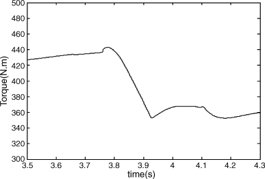
In the inertia phase that follows the torque phase, the main purpose is the synchronization of the engine speed with that of the clutch 2. In fact, this clutch is transmitting the power but with large slips.
The output torque variations during the upshift can be seen in Figure 4.89. No interruption in torque transmission is the advantage of this gearbox during the gearshift.
4.6.3.3 Downshift Performance
A downshift is more complex than an upshift especially at high gears, because in a downshift the on-coming clutch's angular velocity is greater than that of the engine, so that in the absence of suitable synchronization, torque backlash to the engine is very likely. This can cause a large transient in the powertrain system which is undesirable for the vehicle occupants and possibly harmful to the components, especially the gears and shafts. In the downshift case, the subsequent gear is pre-selected and turns with output shaft 1. This time the inertia phase must occur first since the rotational speed of the on-coming clutch (clutch 1) is larger than engine speed and if the clamp force in this clutch is increased, torque will flow in the reverse direction. When the clamp force of the off-going clutch (clutch 2) is decreased, the torque acting on the engine will be reduced, causing the engine to speed up. This will adjust the engine speed closer to the speed of clutch 1 but at the expense of reducing the transmitted torque. In order to maintain the torque and at the same time to accelerate the engine, the throttle can be further opened. This will help to achieve speed synchronization during the inertia phase. During the torque phase the clamp force at the on-coming clutch (clutch 1) is increased and the clamp force at the off-going clutch (clutch 2) is decreased simultaneously until the whole engine torque is transferred through the on-coming clutch. A gear 2 to gear 1 downshift is more severe than the others and a sample downshift performance is shown in Figures 4.90 and 4.91.
Figure 4.90 Angular speeds during downshift from 2nd to 1st gear

Figure 4.91 Transmission output torque during downshift from 2nd to 1st gear

Continuously variable transmissions (CVT) are based on a well-established concept to transmit power from one rotating shaft to another with continuously variable speeds. The basic idea can be understood from a simple arrangement of two similar cones with a flat belt wrapped around them as illustrated in Figure 4.92. As the belt is moved along the parallel axes of the cones, x varies and for a given rotational speed ![]() of input shaft, the output angular speed
of input shaft, the output angular speed ![]() can be obtained by assuming no slip:
can be obtained by assuming no slip:
Figure 4.92 A conceptual CVT

Figure 4.93 depicts the variation of dimensionless output speed ![]() with the variation of dimensionless input displacement
with the variation of dimensionless input displacement ![]() according to Equation (4.228). For a fixed value of input angular speed, the output speed ranges continuously from very small values near zero up to large values. This property of CVTs is useful in many applications in which the benefits of providing different gear ratios in addition to smooth shifting between ratios are required.
according to Equation (4.228). For a fixed value of input angular speed, the output speed ranges continuously from very small values near zero up to large values. This property of CVTs is useful in many applications in which the benefits of providing different gear ratios in addition to smooth shifting between ratios are required.
Figure 4.93 Variation of speed ratio versus displacement ratio

Simple concepts like that of Figure 4.92 may work in some applications, but in automotive applications, due to the high duty cycles and durability requirements only a few types of CVTs have proved successful in practice.
4.7.1 Classification
CVTs used in vehicles may be classified in different ways. The classification shown in the flowchart of Figure 4.94 divides CVTs according to the nature of producing the output torque. Details of each classification will be discussed in the separate sections that follow.
Figure 4.94 A classification for automotive CVTs

4.7.2 Friction CVTs
As the name implies, friction CVTs produce torque based on friction between mating surfaces, by means of belts or rollers. Two types of friction CVTs which are currently used in automobiles are the belt and toroidal CVTs. A belt CVT system is similar to standard belt-pulley drive with the exception that the pulleys are not fixed and are able to move apart. The geometry of a belt type CVT is shown in Figure 4.95. Both pulleys have fixed axes of rotation at a distance C from each other. The sides of each pulley are controlled to move apart or together laterally, but the displacements of each pulley is the opposite of the other. The situation shown in Figure 4.95 is an extreme case when the sides of left pulley are fully apart and sides of right pulley fully closed.
Figure 4.95 Geometry of a typical belt CVT

Assuming no slip between the belt and pulleys, the speed ratio between the drive and driven pulleys can be written as:
(4.229) ![]()
in which x is the distance between the two sides of the drive pulley and:
(4.230) ![]()
(4.231) ![]()
Displacement x is bounded between the two extremes:
(4.232) ![]()
The speed ratio at these extremes is:
(4.233) ![]()
(4.234) ![]()
which are the inverse of each other. Since the trivial condition of ![]() is always satisfied, the speed ratio at
is always satisfied, the speed ratio at ![]() is always larger than its value at
is always larger than its value at ![]() . The speed ratio becomes equal to unity at
. The speed ratio becomes equal to unity at ![]() . In order to increase the overall ratio of the CVT, the difference between the outer and inner radii should be increased. The variation of the speed ratio with the variation of lateral displacement x is illustrated in Figure 4.96 for the special case of
. In order to increase the overall ratio of the CVT, the difference between the outer and inner radii should be increased. The variation of the speed ratio with the variation of lateral displacement x is illustrated in Figure 4.96 for the special case of ![]() .
.
Figure 4.96 Typical variation of speed ratio in belt CVT

The torque transmitted by a standard rubber belt pulley system is through the tensioning of a belt that produces larger tensions in the direction of rotation and small tensions at the loose end (see Figure 4.97 a). The torque, therefore, results from the difference between the tensions at both ends multiplied by the effective radius. Due to the limitations of rubber belts, it is common in automotive applications to use steel belts as the means of transferring torque. One type of such belts is called a ‘push belt’, which in addition to the tension in front end of the belt, produces a compressive (push) force at the trailing end (see Figure 4.97b). This push force contributes to the torque transmission of the CVT. A push belt has a composite structure comprising two major components. One is a series of V-shaped steel segments that, when assembled, resemble a V belt shape. The segments come into contact with the pulleys and bear all contact forces. The other element in a push belt is a number of thin flat steel belt layers that together make a band to stack the segments and constitute a uniform steel belt. These belt layers withstand the tensile forces in the push belt.
Figure 4.97 Rubber belt (a) and push belt (b)

Another friction CVT used in vehicle transmissions is the toroidal type in which free wheels or rollers are placed between cavities of two disks and relate the rotations of two input and output shafts. Figure 4.98 shows the schematics of two variations from this type, namely ‘full toroidal’ and ‘half toroidal’ CVTs. The inside surfaces of the disks are spherical and the wheels or rollers in addition to their spin can oscillate laterally and change the radii of the contact points of input and output disks and in turn the speed ratio of the CVT.
Figure 4.98 Full toroidal (a) and half toroidal (b) CVT types

One of main problems in friction CVTs is the friction generated at the contacting points. Friction is used to generate traction forces at the contact region which in turn generates a torque. But friction has two problems: build-up of heat and sensitivity to wear. In order to resolve these problems, lubricating oil can be used but this will reduce the friction and torque capacity of the CVT. The friction force depends on the coefficient of friction and normal load. Increase in normal load can compensate for the reduction of coefficient of friction provided that the oil can withstand high pressures and temperatures. Special traction oils have the required properties and are used for this purpose.
4.7.3 Ratcheting CVTs
A ratchet is a device that produces rotation in one direction regardless of the direction of the input rotation. This produces an intermittent output from a non-uniform and even oscillatory input. Ratcheting gearboxes are based on the concept of producing the output rotation from a series of discontinuous rotations summed up at the output. For this purpose the gearbox is constructed from a number of similar mechanisms. In order to understand the concept, consider a four-bar mechanism shown in Figure 4.99. If a constant input angular speed ωi is applied to the mechanism, an output angular speed ωo will result. Depending on the geometry, the output could be similar to that shown in Figure 4.100 in normalized form (i.e., ωo divided by ωi). Since the output in a gearbox must rotate in the same direction of the input, only positive parts of the output are acceptable. In addition, the gearbox should have a fixed ratio with rotation of the input shaft.
Figure 4.99 A four-bar mechanism

Figure 4.100 The normalized output speed of a typical four-bar mechanism

If several mechanisms of equal geometry are used in such a way that their input linkages are connected to the same input shaft in timed angles, several of output angular speeds will be available as shown in Figure 4.101 for only four mechanisms. Now if one-way clutches (or free wheels) are used at the outputs, in such a way that at certain moments each clutch engages and disengages, the overall output of the system will look like that shown in Figure 4.102. This output, although irregular (similar to engine output torque irregularities), has an average and can be used in practice as a gearbox output.
Figure 4.101 Outputs of several mechanisms

Figure 4.102 Output of the system with one-way clutches

The four-bar linkage was only an example of how a mechanism can be used to build a gearbox, several other mechanisms have this potential and some might perform better. For example, if the output of a mechanism at a certain span of input angles is almost flat, then the gearbox output from such a mechanism is more desirable and fewer mechanisms are necessary to build the gearbox. This explanation shows how a gearbox can be constructed, but the main issue is whether it can act as a CVT. To this end if the mechanism can be altered during the work, the gearbox will change ratio and a CVT characteristic can result. Consider, for instance, the same four-bar mechanism of Figure 4.99, but with an adjustable input arm depicted in Figure 4.103. Changing the input arm length will change the speed ratio of the mechanism and if it is done continuously, a CVT is effectively achieved.
Figure 4.103 A four-bar mechanism with adjustable input arm

4.7.4 Non-Mechanical CVTs
Two important types of non-mechanical CVTs are based on hydraulic and electrical components. A hydraulic system comprising a pump and a hydraulic motor constitutes a gearbox, since the pump produces oil flow and turns the motor. Thus the input mechanical power is first transformed to fluid power by the pump and once again to mechanical power by the motor. Converting such a system to a CVT is done simply by selecting the pump and/or motor of variable displacement type. Figure 4.104a shows a simplified representation of a hydraulic CVT in which the engine (E) rotates the variable displacement pump (P). The fluid is sucked from tank (T) to the pump and fed to the hydraulic motor (HM) and returned to the tank again. Such a system is referred to as a hydrostatic transmission and has been used successfully in off-road vehicle applications.
Figure 4.104 Non-mechanical CVT types (a) hydraulic and (b) electrical

An electric system consisting of a generator and a motor is quite similar to the hydraulic gearbox. The mechanical input power can rotate the generator and produce electric current that in turn can drive an electric motor and produce mechanical power at the output. Converting this system to a CVT is achieved by using electric power circuits that control the motor's voltage (or frequency). Figure 4.104b schematically shows an electrical system consisting of a generator (G) and an electric motor (M) connected by a controller.
Although these systems may look very simple and practical, nevertheless due to heavy weights and power losses resulting from double energy transformation involved, they have not been widely used in automobile applications. However, with the remarkable growth of interest in electric vehicles in the early years of the twenty-first century, this situation is set to change.
4.7.5 Idling and Launch
Interruption of torque from the engine to the driveline is necessary when the vehicle is at rest with the engine running. For manual transmissions a clutch disconnects the torque but it is not enough on its own and the gearbox must have a neutral condition to allow idling comfortably when clutch is released. For vehicle launch from standstill, the clutch allows the engagement of the necessary gear and then acceleration is achieved by releasing the clutch. In automatic transmissions the torque converter makes both the idling and launch possible. For most CVTs there are a range of gear ratios between the upper and lower values and the torque interruption from the engine is necessary at idling. This needs an additional device such as a torque converter or friction clutch. The launch from standstill can also be handled with such device. Some CVT systems produce gear ratios ranging from zero to the highest ratio. The zero ratio makes idling possible as there is no (zero) torque transfer from engine at this particular gear ratio (neutral). These systems are called infinitely variable transmissions (IVT).
This chapter covered aspects of the transmission design including gear ratios, tooth numbers, clutch torque capacity and dynamics. Gearbox ratio estimation was divided into three parts of low, high and intermediate gears and several methods for the determination of ratios were discussed. The evaluation of the dry clutch torque delivering capacity was studied and design issues were discussed. Useful semi-empirical equations provided for the clutch force (MG formula) to facilitate analytical solutions as well as more realistic simulations of clutch engagement. The clutch dynamics were simulated in some detail, although this particular subject has attracted further detailed attention particularly in relation to DCT designs.
The construction and basics of operation of transmissions were considered and the differences between manual and automatic transmissions were summarized. Automatic transmissions comprising the conventional automatics and automated manuals (AMTs) were described. The recent developments of DCT transmissions as improved versions of AMTs was explained and the DCT performance during the upshift and downshift actions was discussed. Further details on the quality of shiftings involve the control of clutch forces, slips and throttle regulation. CVTs were described and classified and an overview of the functioning of different types was provided. More advanced subjects such as DCT and CVT dynamics and control are beyond the scope of this book.
4.1 Explain the reasons why a gearbox is needed for the vehicle. When would it be possible to use only one reduction gear?
4.2 Why are the design methods for the lowest and highest transmission gear ratios different?
4.3 Describe the method of designing the lowest gear in the transmission.
4.4 Explain the factors on which the gradeability of the vehicle at low speed depends.
4.5 Describe the method of designing the highest gear in the transmission.
4.6 Explain how to design the highest gear to achieve the maximum possible vehicle speed.
4.7 A student proposes a design method in which the intermediate gears are evenly spaced between the lower and higher gear ratios. What is wrong with this suggestion?
4.8 What is the idea behind the geometric progression method?
4.9 Describe the progressive design method of intermediate gear ratios.
4.10 How does the equal ΔV method differ from the progressive method?
4.11 Describe the two types of meshing in manual transmissions.
4.12 In manual transmissions explain why synchronization is necessary and how is it performed.
4.13 What is the difference between the transaxle and layshaft manual transmissions?
4.14 The first student says that the gears inside a manual transmission stop rotating once the clutch is depressed. The second student believes the gears will stop only when the transmission is in neutral. Which student is correct?
4.15 In friction clutches describe the two criteria for the pressure distribution and their justification.
4.16 Compare the torque capacity of a dry clutch at both working conditions and discuss which case is more appropriate for clutch design.
4.17 Describe the operation of a friction clutch system by drawing a schematic figure.
4.18 Explain why the clutch plate is released when the release bearing is pressed towards the engine.
4.19 A student believes the pedal force of a clutch is at maximum when the clutch is new and linings are thick. What is your comment?
4.20 Explain how the clamp force of the clutch varies when the pedal is depressed.
4.21 Explain how it is possible to have the clutch torque larger than the input engine torque.
4.22 Describe the construction of manual and conventional automatic transmissions.
4.23 Describe the operation of a torque converter.
4.24 A student suggests using a torque converter in manual transmissions to replace the clutch. Does this work?
4.25 Explain why several planetary gear sets are required in conventional automatics.
4.26 Describe the method of gear selection in conventional automatics.
4.27 Describe the method of converting a manual to an AMT. What are the advantages of AMTs over manuals and conventional automatics?
4.28 What is the main difference between a DCT and an AMT? What are the advantages of DCTs over the conventional automatics?
4.29 Describe the operation of a DCT.
4.30 Explain why the upshift and downshift controls are different in a DCT.
4.31 Describe the classification of CVTs and specify which types are used in practice.
Problem 4.1
Explain why the term Nf + Nr of Equations (4.19) and (4.20) is not necessarily equal to Wcosθ and discuss the conditions of equality.
Problem 4.2
Repeat Example 4.3.2 and show that for lower adhesion coefficients of below 0.7, FWD vehicle can have better gradeability results than RWD vehicle.
Problem 4.3
For a vehicle with information given in Table P4.3:
(a) Find an expression for the overall high gear ratio for the case in which the maximum vehicle speed occurs at the engine speed corresponding to the maximum engine torque.
(b) Repeat (a) for the case where the maximum vehicle speed occurs at the engine speed corresponding to the maximum engine power.
Result: (a) ![]()
Table P4.3 Vehicle information of Problem 4.3.
| 1 | Aero drag coefficient | c |
| 2 | Rolling resistance coefficient | f |
| 3 | Tyre rolling radius | R |
| 4 | High gear ratio | n |
| 5 | Maximum engine torque | |
| 6 | Engine speed at max torque | |
| 7 | Torque at max engine power | |
| 8 | Engine speed at max power | |
| 9 | Vehicle mass | m |
Problem 4.4
For the vehicle in Example 4.3.3 design the highest gear ratio in the manner described below and compare the result with those of Examples 4.3.3–4.3.4.
First design gear 4 at the engine speed 10% above the speed at the maximum power and then design gear 5 with a 25% overdrive.
Problem 4.5
Prove Equation (4.37) for the overdrive gear ratio by writing the kinematic equation of vehicle motion. State the assumptions involved in this process.
Problem 4.6
In a 4WD vehicle the wheel torques at front and rear axles are distributed such that the ratio of front to rear axle torques is given by r.
(a) Assume the rear wheels are at the point of slip and derive an expression for the maximum negotiable slope of the vehicle (assume equal gear ratios for front and rear and ignore the rolling resistance).
(b) Repeat (a) assuming the front wheels are at the point of slip.
(c) For both cases of (a) and (b) derive expressions for the limits of torque ratio r.
(d) Use numerical values 2.5, 0.5, 1.2, 0.8 and 0.02 for l, h, a, μ and fR to evaluate the limits of r.
Result: (a) ![]() (d) r ≤ 0.57 and r ≥ 0.57
(d) r ≤ 0.57 and r ≥ 0.57
Problem 4.7
A method shown in Figure 4.105 is proposed for the evaluation of intermediate gearbox ratios. It includes two low speed levels for the engine with the definition of ![]() (
(![]() ).
).
Figure P4.7 Engine-vehicle speed diagram of Problem 4.7

(a) Find expressions for ![]() and
and ![]() .
.
(b) Find expressions for ![]() ,
, ![]() and
and ![]() in terms of
in terms of ![]() .
.
(c) Examine the difference between the average of ![]() and
and ![]() with
with ![]() of geometric progression.
of geometric progression.
(d) Show that for ![]() this method is identical to conventional geometric progression.
this method is identical to conventional geometric progression.
Results: (a) ![]() and
and ![]() .
.
Problem 4.8
A method is proposed for the evaluation of intermediate transmissions ratios presented in Figure P4.8. With the assumption of ![]() (
(![]() ),
), ![]() ,
, ![]() .
.
Figure P4.8 Engine-vehicle speed diagram of Problem 4.8

(a) Find an expression for the calculation of ![]() in terms of N and t (or α).
in terms of N and t (or α).
(b) Find expressions for ![]() ,
, ![]() and
and ![]() in terms of known parameters.
in terms of known parameters.
(c) Show that for ![]() the above results are identical to conventional geometric progression.
the above results are identical to conventional geometric progression.
Result: (a) ![]()
Problem 4.9
Repeat Problem 4.8 for the following engine-vehicle speed diagram in Figure P4.9.
Figure P4.9 Engine-vehicle speed diagram of Problem 4.9

Result: (a) ![]()
10.10 Problem 4.10
In a vehicle clutch, the inner and outer disk radii are r and R respectively, while the maximum spring force is ![]() .
.
(a) Write an expression for ΔT, the difference between delivered torque at the two cases of constant pressure and uniform wear in terms of the uniform wear torque.
(b) Calculate the ratio ![]() for the three cases of ΔT = 1%, 5% and 10% of the torque of constant wear.
for the three cases of ΔT = 1%, 5% and 10% of the torque of constant wear.
(c) Draw the variation of ΔT/Tuw versus ![]() .
.
Result: (b) ![]() .
.
Problem 4.11
For the clutch of Problem 4.10:
(a) Is there an answer for r for having equal torques at both cases of uniform pressure and uniform wear? Explain why.
(b) With ![]() being the coefficient of friction, find an expression for the maximum difference between the clutch torques in the two cases.
being the coefficient of friction, find an expression for the maximum difference between the clutch torques in the two cases.
Result: (b) ![]() .
.
Problem 4.12
If the sum of groove angles on the clutch plate lining is θ (radians), show that the actual maximum pressure on the material is ![]() times its theoretical value with no grooves, for both uniform pressure and uniform wear.
times its theoretical value with no grooves, for both uniform pressure and uniform wear.
Problem 4.13
During the clutch release in gear 1, the clutch force is increased linearly from zero to the maximum of 5000 N. The variations of the engine and clutch rotational speeds are of the form shown in Figure P4.13.
Figure P4.13 Engine-clutch speed diagram of Problem 4.13

For information given in Table P4.13, determine the clutch efficiency.
Table P4.13 Information for Problem 4.13.

Problem 4.14
The driver of a vehicle decides to gearshift from gear 1 to gear 2 when the travelling speed reaches 36 km/h. At the time driver releases the clutch pedal the engine is idling.
(a) Determine the rotational speeds of engine, clutch plate and driving wheels at the time the clutch starts to be released (use Table P4.14).
(b) Specify the torque flow direction if the driver:
(i) just releases the clutch pedal;
(ii) increases the engine speed before releasing the clutch pedal.
(c) Plot a rough variation of the engine and clutch plate speeds versus time during the gearshift for two cases when the driver attempts to:
(i) accelerate right after gearshift;
(ii) maintain a uniform speed.
(d) Is it possible to gearshift without using the clutch? Explain how.
Result: (a) ![]() ,
, ![]() and
and ![]() .
.
Table P4.14 Information for Problem 4.14.
| Engine idle speed | 1000 rpm |
| Tyre rolling radius | 33 cm |
| Overall ratios at 1st, 2nd and 3rd gears | 14, 9 and 6 |
Problem 4.15
For a 4WD vehicle the CG is at equal distances from the front and rear axles and the CG height to the ground is half of the same distance. For μP = 1, assume equal driveline efficiencies for driving with front or rear wheels and determine the ratio of FWD to RWD low gear ratios
![]()
Result: k ≈0.6.
Problem 4.16
The gear ratio of a layshaft gearbox in gear 1 is 3.85:1. Two options with sub-ratio combination 1.75 × 2.2 and 1.925 × 2 are proposed for the determination of tooth numbers (in each case the left figure is input gear mesh ratio and the second figure is the output gear mesh ratio). The distance between the centrelines of the upper and lower shafts has to be larger than 100 mm but as small as possible. Gear modules must be larger than 1mm with spacing of 0.25 mm (e.g. 1.25, 1.50, etc.). Find the tooth numbers for all four gears for both given options and select the best answer.
Problem 4.17
For the vehicles with given properties in Table P4.17:
(a) Determine the maximum grade each vehicle can climb.
(b) At the grade found in (a), what percentage of maximum engine power is utilized at speed of 30 km/h?
(c) At the grade found in (a), what percentage of maximum engine torque is utilized at speed of 30 km/h?
Table P4.17 Vehicle information of Problem 4.17.

Problem 4.18
The information for a passenger car clutch spring is given in Table P4.18:
(a) Plot the FS-δS and FB-δB curves using the MG formulae.
(b) Calculate the seesaw gain ks.
(c) Plot the variation of clamp force inside the first plot of FS-δS.
(d) Calculate the initial deflection ![]() .
.
Table P4.18 Clutch information of Problem 4.18.
| Parameter | Value | Unit |
| Inner diameter Di | 34 | mm |
| Outer diameter Do | 185 | mm |
| Bellville inner diameter Db | 151 | mm |
| Spring thickness t | 2.3 | mm |
| Bellville height h | 3.4 | mm |
| Set point deflection |
3.4 | mm |
| Modulus of elasticity | 206 | MPa |
| Poisson's ratio | 0.3 | – |
Problem 4.19
For the vehicle with given specifications in Table P4.19.1, the engine is off. For the two cases of uphill and downhill, determine the maximum grade vehicle can stop without slipping, if:
(a) only gear 1 is engaged;
(b) only the handbrake on the front wheels is activated;
(c) only the handbrake on the rear wheels is activated;
(d) only the footbrake is activated;
(e) gear 1 is engaged together with the handbrake acting on front wheels;
(f) gear 1 is engaged together with the handbrake acting on rear wheels.
Compare the results for both cases of FWD and RWD by filling in Table P4.19.2.
Table P4.19.1 Vehicle information of Problem 4.19.

Table P4.19.2 Proposed table for filling in the results.

Problem 4.20
The intention is to investigate the existence of a certain grade and friction coefficient for which both FWD and RWD vehicles with same properties generate equal traction forces.
(a) In the expression for the tractive forces of FWD and RWD vehicles ignore the hfR term and find a condition for friction coefficient which guarantees equal traction forces for the both cases.
(b) Using the result of (a) prove that for both cases: ![]() .
.
(c) Use ![]() and
and ![]() and calculate the values of μP and θ.
and calculate the values of μP and θ.
(d) Retain the hfR term and repeat case (a) and show that the result in (b) is still valid and that the friction coefficient must satisfy the condition: ![]() if values in (c) are used.
if values in (c) are used.
Problem 4.21
In the expressions for the tractive forces of FWD and RWD vehicles, ignore the hfR term and derive equation for slope in the form of ![]() and then:
and then:
(a) Find values c, d and e for both cases given ![]() and
and ![]() .
.
(b) From a mathematical point of view investigate the possibility of a maximum grade each type of vehicle can negotiate by differentiating θ with respect to μP and find θmax for each case.
(c) Draw the variation of θ versus μP for both cases (evaluate θ values for μP up to 4).
(d) What would be the values of θmax for each case in the real practice? (Suggest a practical μmax.)
Problem 4.22
In the derivation of Equations (4.212) and 213 the limitation on the clutch torque was not included. Derive the equations for the clutch efficiency when considering this limitation.
In contrast to the enormous number of books on engines, textbooks devoted to transmissions are relatively rare. It is not clear why this huge discrepancy has occurred – particularly since developments in transmissions have had a major impact on vehicle design, especially over recent years – and yet informative texts on multispeed automatics, dual clutch transmissions and CVTs are not available.
The best introduction to automotive transmissions is probably Chapter 13 in Happian Smith (ed.), written by Vaughan and Simner [10]. They provide an excellent overview of the fundamentals of transmissions and describe the functional aspects of different components without going into the analysis. Details of gear design and manual gearbox design are provided in Stokes' 1992 texts [11, 12].
Other useful descriptive material is available in Heisler [13] and Gott [14] but both these texts are now dated and do not cover any of the interesting developments over the past two decades. The most comprehensive text on automotive transmissions is by Naunheimer et al. [15] which is a recent update of an earlier 1999 book [2]. It is aimed more at the practising professional engineer than the student market and so it remains rather expensive. However, it is a definitive text; as well as covering the basic vehicle performance, it also provides detailed design information on gears, shafts, bearings and synchronizers. It describes manual, automatic gearboxes and torque converters and introduces overall aspects of the commercial design, development and testing processes associated with transmission manufacture.
[1] Wong, J.Y. (2001) Theory of Ground Vehicles, 3rd edn. John Wiley & Sons, Inc., ISBN 0-470-17038-7.
[2] Lechner, G. and Naunheimer, H. (1999) Automotive Transmissions: Fundamentals, Selection, Design and Application. Springer, ISBN 3-540-65903-X.
[3] Shigley's Mechanical Engineering Design, 8th edn. McGraw-Hill, 2006, ISBN 0-390-76487-6.
[4] Mabie, H.H. and Reinholtz, C.F. (1987) Mechanisms and Dynamics of Machinery, 4th edn. John Wiley & Sons, Inc. ISBN 0-471-02380-9.
[5] Lhomme, W. et al. (2008) Switched Causal Modeling of Transmission with Clutch in Hybrid Electric Vehicles, IEEE Transactions on Vehicular Technology, 57 (4).
[6] Berger, E.J. (2002) Friction Modeling for Dynamic System Simulation, Applied Mechanics Review, 55 (6): 535–577.
[7] Duan, C. (2004) Dynamic Analysis of Dry Friction Path in a Torsional System. PhD dissertation, The Ohio State University.
[8] Amari, R., Tona, P. and Alamir, M. (2009) A Phenomenological Model for Torque Transmissibility During Dry Clutch Engagement, paper presented at 18th IEEE International Conference on Control Applications, Saint Petersburg, Russia, July.
[9] Newbold, D. and Bonnick, A.W.M. (2005) A Practical Approach to Motor Vehicle Engineering and Maintenance. Elsevier Butterworth-Heinemann, ISBN 0-7506-6314-6.
[10] Happian Smith, J. (ed.) (2002) An Introduction to Modern Vehicle Design. Butterworth-Heinemann, ISBN 07506-5044-3.
[11] Stokes, A. (1992a) Gear Handbook: Design and Calculations. Butterworth-Heinemann, ISBN 07506-149-9.
[12] Stokes, A. (1992b) Manual Gearbox Design. Butterworth-Heinemann, ISBN 07506 0417 4.
[13] Heisler, H. (2002) Advanced Vehicle Technology, 2nd edn. Butterworth Heinemann, ISBN 07506-5131-8.
[14] Gott, P.G. (1991) Changing Gears: The Development of the Automatic Transmission. SAE, ISBN 1-56091-099-2.
[15] Naunheimer, H., Bertsche, B., Ryborz, J., Novak, W., Fietkau, P. and Kuchle, A. (2010) Automotive Transmissions: Fundamentals, Selection, Design and Application, 2nd edn. Springer, ISBN 978-3642162138.