
12
CORDIC-based DDFS
Architectures
12.1 Introduction
This chapter considers the hardware mapping of an algorithm to demonstrate application of the techniques outlined in this book. Requirement specifications include requisite sampling rate and circuit clock. A folding order is established from the sampling rate and circuit clock. To demonstrate different solutions for HW mapping, these requirements are varied and a set of architectures is designed for these different requirements.
The chapter explores architectures for the digital design of a direct digital frequency synthesizer (DDFS). This generates sine and cosine waveforms. The DDFS is based on a CoORDinate DIgital Computer (CORDIC) algorithm. The algorithm, through successive rotations of a unit vector, computes sine and cosine of an input angle θ.Each rotation is implemented by a CORDIC element (CE). An accumulator in the DDFS keeps computing the next angle for the CORDIC to compute the sine and cosine values. An offset to the accumulator in relation with the circuit clock controls the frequency of the waveforms produced.
After describing the algorithm and its implementation in MATLAB®, the chapter covers design techniques that can be applied to implement a DDFS in hardware. The selection is based on the system requirements. First, a fully dedicated architecture (FDA) is given that puts all the CEs in cascade. Pipelining is employed to get better performance. This architecture computes new sine and cosine values in each cycle. If more circuit clock cycles are available for this computation then a time-shared architecture is more attractive, so the chapter considers time-shared or folding architectures. The folding factor defines the number of CEs in the design. The folded architecture is also pipelined to give better timings.
Several novel architectures have been proposed in the literature. The chapter gives some alternate architecture designs for the CORDIC. A distributed ROM-based CORDIC uses read-only memory for initial iterations. Similarly, a collapsed CORDIC uses look-ahead transformation to merge several iterations to optimize the CORDIC design.
The chapter also presents a novel design that uses a single iteration to compute the values of sine and cosine, to demonstrate the extent to which a designer can creatively optimize a design.
12.2 Direct Digital Frequency Synthesizer
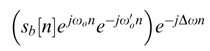
A DDFS is an integral component of high-performance communication systems [1]. In a linear digital modulation system like QAM, the baseband signal is translated in frequency. This translation is usually done in more than one stage. The first stage of mixing is performed in the digital domain and a complex baseband signal sb[n] is translated to an intermediate frequency (IF) by mixing it with an exponential of equivalent digital frequency ωo:
This IF signal is converted to analog using a D/A converter and then mixed using analog mixers for translation to the desired frequency band.
At the receiver the similar complex mixing is performed. The mixer in the digital domain is best implemented using a DDFS. Usually, due to differences in the crystals for clock and frequency generation at the transmitter and receiver, the mixing leaves an offset :(12.2)
The receiver needs to compute this frequency error, the offset being Δω =ωo– ω'o.The computation of correction is made in a frequency correction loop. The frequency adjustment again requires generation of an exponential to make this correction. A DDFS is used to generate the desired exponential:
A DDFS generates a spectrally pure sine and cosine for quadrature mixing and frequency and phase correction in a digital receiver, as shown in Figure 12.1. At the front end, a DDFS mixes with the digitized IF signal. The decimation stage down-converts the signal to baseband. The phase detector computes the phase error and the output of the loop filter generates phase correction for DDFS that generates the correction for quadrature mixing.
Figure 12.1 Use of DDFS in a digital communication receiver
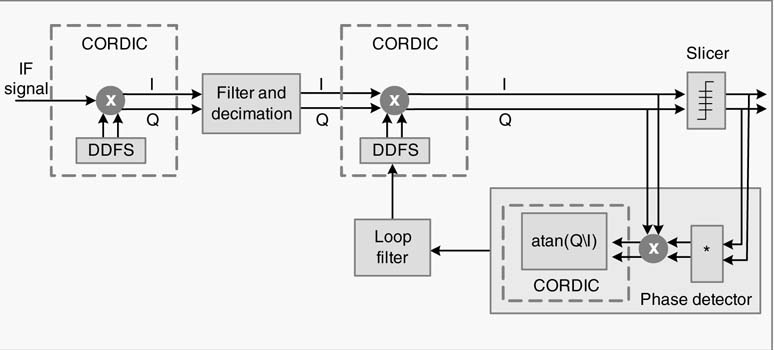
For a high data-rate communication system, this value needs to be computed in a single cycle. In designs where multiple cycles are available, a folded and time-shared architecture is designed to effectively use area. Similarly, while demodulating an M-ary phase-modulated signal, the slicer computes tan–1(Q/I), where Q is the quadrature and I is the in-phase component of a demodulated signal. All these computations require an effective design of CORDIC architecture.
A DDFS is also critical in implementing high-speed frequency and phase modulation systems as it can perform fast switching of frequency at good frequency resolution. For example, a GMSK baseband modulating signal computes the expression [2]:
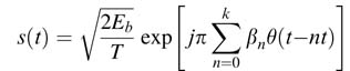
for kT<t<(k + 1)T,where T is the symbol period, Eb is the energy per bit, βn ∈{1,– 1} is the modulating data, and θ(t) is the phase pulse. A DDFS is very effective in generating a baseband GMSK signal.
A DDFS is characterized by its spectral purity. A measure of spectral purity is the ‘spurious free dynamic range’ (SFDR), defined as the ratio (in dB) of amplitude of the desired frequency to the highest frequency component of undesired frequency.
12.3 Design of a Basic DDFS
A simple design of a DDFS is given in Figure 12.2. A frequency control word W in every clock cycle of frequency fclk is added in an N-bit phase accumulator. If W =1, it takes the clock 2N cycles to make the accumulator overflow and starts again. The output of the accumulator is used as an address to a ROM/ RAM where the memory stores a complete cycle of a sinusoid. The data from the memory generates a sinusoid. The DDFS can generate any frequency fo by an appropriate selection of W using:
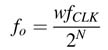
The digital signals cos(ωon) and sin(ωon) can be input to a D/A converter at sampling rate T=1/fCLK for generating analog sinusoids of frequency fo, where:
The maximum frequency from the DDFS is constrained by the Nyquist sampling criterion and is equal to fclk/2.
The basic design of Figure 12.2 is improved by exploiting the symmetry of sine and cosine waves.
Figure 12.2 Design of a basic DDFS
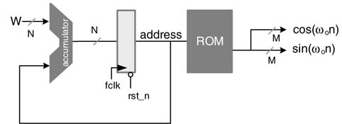
Figure 12.3 Design of a DDFS with reduced ROM size
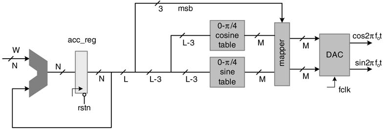
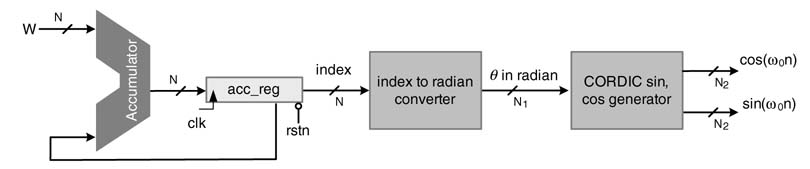
Figure 12.4 DDFS with CORDIC block for generating sine and cosine of an angle θ
The modified design is shown in Figure 12.3. The output of the accumulator is truncated from N to L bits to reduce the memory requirement. A complete period 0 to 2π of sine and cosine waves can be generated from values of the two signals from 0 to π/4.The sizes of the two memories are reduced by one-eighth by only storing the values of sine and cosine from 0 to π/4. The L–3 bits are used to address the memories, and then three most signficant bits (MSBs) of the address are used to map the values to geneheta value must be within -0.9579 and 0.9579 radians rate complete periods of cosine and sine.
A ROM/RAM-based DDFS requries two 2L–3 deep memories of width M. The design takes up a large area and dissipates significant power. Several algorithms and techniques have been proposed that reduce or completely eliminate look-up tables in memories. An efficient algorithm is CORDIC, which uses rotation of vectors in Cartesian coordinates to generate values of sine and cosine.
The DDFS with a CORDIC block is shown in Figure 12.4. The CORDIC algorithm takes angle θin radians, whereas the DDFS accumulator specifies the angle as an index value. To use a CORDIC block in DDFS, a CSD multiplier is required that converts index n to angle θin radians, where:
12.4 The CORDIC Algorithm
12.4.1 Introduction
This algorithm was originally developed by Volder in 1959 to compute the rotation of a vector in the Cartesian coordinate system [3]. The method has been extended for computation of hyperbolic functions, multiplication, division, exponentials and logarithms [4].
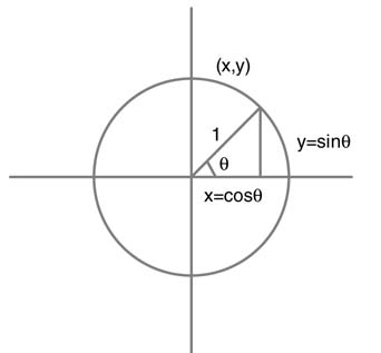
Figure 12.5 The CORDIC algorithm successively rotates a unit vector to desired angle θ
Multiplication by sine and cosine is an integral part of any communication system, so area- and time-efficient techniques for iterative computation of CORDIC are critical. The best application of the CORDIC algorithm is its use in DDFS. Several architectural designs around CORDIC have been reported in the literature [5-8].
To bring a unit vector to desired angle θ, the basic CORDIC algorithm gives known recursive rotations to the vector. Once the vector is at the desired angle, then the x and y coordinates of the vector are equal to cos θand sin θ, respectively. This basic concept is shown in Figure 12.5.
Mathematically the angle θ is approximated by addition and subtraction of angles of N successive rotations Δθi. The expression for the approximation is:
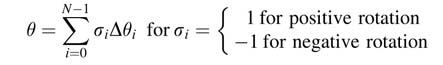
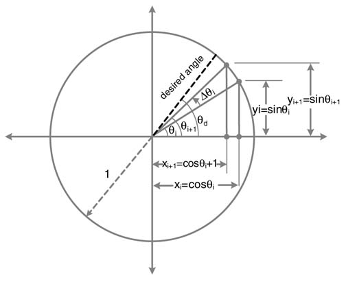
As depicted in Figure 12.6, the unit vector in iteration i is rotated by some angle θi and the next rotation is made by an angle Δθi that brings the vector to new angle θi+1, then:
From the figure it can be easily established that xi=cos θi, yi=sin θi and similarly xi+1= cos θi+1, yi+1, yi+1 = sin θi+1.Substituting these in (12.6) we get:
In matrix forms, the set of equations in (12.7) can be written as:
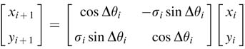
Figure 12.6 CORDIC algorithm incremental rotation by Δθi
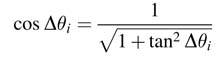
Taking cosΔθi common yields:
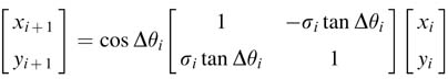
In this expression cos Δθi can also be written in terms of tan Δθi as:
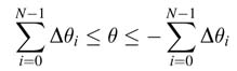
To avoid multiplication in computing (12.8), the incremental rotation is set as:
which implies Δθi=tan–1 2 –i, and the algorithm applies N such successive micro-rotations of ±Δθi to get to the desired angle θ. This arrangement also poses a limit to the desired angle as:
Now substituting expression (12.9) in (12.8) gives:
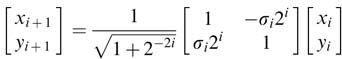
This can be written as a basic rotation of the CORDIC algorithm:
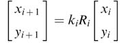
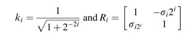
where
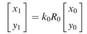
Starting from index i = 0, the expression in (12.10) is written as:
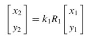
and for index i = 1 the expression becomes:
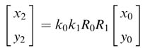
Now substituting the value of ![]() from (12.11a) into this expression, we get:
from (12.11a) into this expression, we get:
Writing (12.10) for indices i =3,4,….,N – 1 and then substituting values for the previous indices, we get:
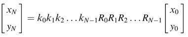
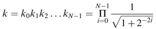
All the ki are constants and their product can be pre-computed as constant k, where:
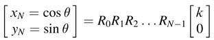
For each stage or rotation, the algorithm computes σi to determine the direction of the ith rotation to be positive or negative. The factor k is incorporated in the first iteration and the expression in (12.12) can then be written as:
12.4.2 CORDIC Algorithm for Hardware Implementation
For effective HW implementation the CORDIC algorithm is listed as follows:
S0 To simplify the hardware, θ0 is set to the desired angle θd and θ1 is computed as:
where σ0 is the sign of θ0. Also initialize x0= k and y0=0.
S1 The algorithm then performs N iterations for i =1,…, N –1, and performs the following set of computations:
All the values for tan–1 2–i are pre-computed and stored in an array.
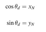
S2 The final iteration generates the desired results as:
The following MATLAB® code implements the CORDIC algorithm:
% CORDIC implementation for generating sin and cos of desired angle
% theta_d
close all
clear all
clc
% theta resolution that determines number of rotations of CORDIC
% algorithm
N = 16;
% generating a tan table and value of constant k
tableArcTan = [];
k = 1;
for i=1:N
 k = k * sqrt(1+(2^(-2*i)));
 tableArcTan = [tableArcTan atan(2^(-i))];
end
x = zeros(1,N+1);
y = zeros(1,N+1);
theta = zeros(1,N+1);
% Tine = [];
cosine = [];
% Specify all the values of theta
theta_s = -0.9;
theta_e = 0.9;
for theta_d = theta_s:.1:theta_e
% CORDIC algorithm starts here
theta(1) = theta_d;
x(1) = k;
y(1) = 0;
for i=1:N,
 if (theta(i) > 0)
 sigma = 1;
 else
 sigma = -1;
end
x(i+1) = x(i) - sigma*(y(i) * (2^(-i)));
y(i+1) = y(i) + sigma*(x(i) * (2^(-i)));
theta(i+1) = theta(i) - sigma*tableArcTan(i);
end
% CORDIC algorithm ends here and computes the values of
% cosine and sine of the desired angle in y(N+1) and
% x(N+1), respectively
cosine = [cosine x(N+1)];
sine = [sine y(N+1)];
end
Figure 12.7 shows output of the MATLAB® code that correctly computes values of sine and cosine using the basic CORDIC algorithm. The range of angle θis from –0.9 radians (–54.88 degrees) to 0.9 radians (54.88 degrees).
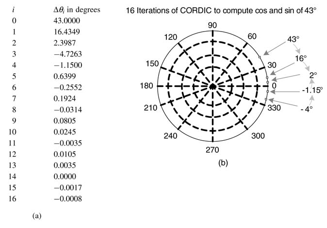
One instance of the algorithm for θ = 43 degrees is explained in Figure 12.8. The CORDIC starts with θ0=43. As CORDIC tries to make the resultant angle equal to 0 it applies a negative rotation Δθ0= tan–12–0 to bring the angle θ1=16.44. Two more negative rotations take the angle to the negative side with θ3= –4.73. The algorithm now gives positive rotation Δθ3=tan –12–3 and keeps working to make the final angle equal to 0, and in the final iteration the angle θ16=–0.0008 degrees.
Figure 12.7 Computation of sine and cosine using basic CORDIC algorithm
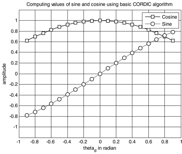
Figure 12.8Example of CORDIC computing sine and cosine for θ = 43 degrees. (a)Table of values of θ ifor every iteration of the CORDIC algorithm. (b) Plot showing convergence
12.4.3 Hardware Mapping
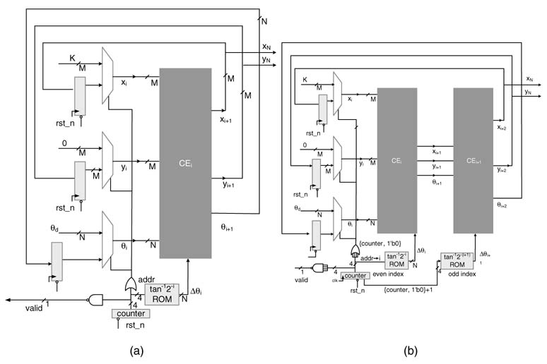
The CORDIC algorithm exhibits natural affinity for HW mapping. Each iteration of the algorithm can be implemented as a CORDIC element (CE). A CE is shown in Figure 12.9(a). This CE implements ith iteration of the algorithm given by (12.14) and is shown in Figure 12.9(b).
Figure 12.9 Hardware mapping. (a) ACORDIC element. (b)An element implementing the ith iteration of the CORDIC algorithm
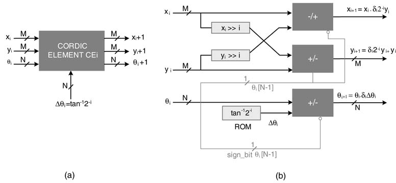
Figure 12.10 FDA architecture of CORDIC as cascade of CEs
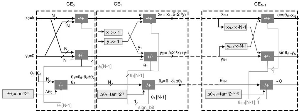
Figure 12.11 Pipelined FDA architecture of CORDIC algorithm
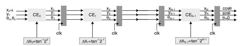
These CEs are cascaded together for a fully parallel implementation. This mapping is shown in Figure 12.10. This design can also be pipelined for better timing. A pipelined version of the fully parallel design is shown in Figure 12.11.
This pipeline structure for CORDIC is very regular and its implementation in Verilog is given below. The code is compact as it uses the for loop statement for generating multiple instances of CEs and pipeline registers.
module CORDIC #(parameter M = 22, N = 16, K=22’h0DBD96)
// In Q2.20 format value of K = 0.8588
(
input signed [N - 1:0] theta_d,
input clk,
input rst_n,
output signed [M - 1:0] cos_theta,
output signed [M - 1:0] sine_theta);
reg signed [M-1:0] x_pipeline [0:N-1];
reg signed [M-1:0] y_pipeline [0:N-1];
reg signed [N-1:0] theta_pipeline [0:N-1];
reg signed [M-1:0] x[0:N];
reg signed [M-1:0] y[0:N];
reg signed [N-1:0] theta[0:N];
reg signed [N-1:0] arcTan[0:N-1];
integer i;
// Arctan table: radian values are represented in Q1.15 format
always @*
begin
 arcTan[0] = 16’h3B59;
 arcTan[1] = 16’h1F5B;
 arcTan[2] = 16’h0FEB;
 arcTan[3] = 16’h07FD;
 arcTan[4] = 16’h0400;
 arcTan[5] = 16’h0200;
 arcTan[6] = 16’h0100;
 arcTan[7] = 16’h0080;
 arcTan[8] = 16’h0040;
 arcTan[9] = 16’h0020;
 arcTan[10] = 16’h0010;
 arcTan[11] = 16’h0008;
 arcTan[12] = 16’h0004;
 arcTan[13] = 16’h0002;
 arcTan[14] = 16’h0001;
 arcTan[15] = 16’h0000;
end
always @*
begin
 x[0] = K;
 y[0] = 0;
 theta[0] = theta_d;
 CE_task(x[0], y[0], theta[0], arcTan[0], 4’d1, x[1],y[1], theta[1]);
 for (i=0; i<N-1; i=i+1)
 begin
 CE_task(x_pipeline[i], y_pipeline[i], theta_pipeline[i],
 arcTan[i+1], i+2, x[i+2], y[i+2], theta[i+2]);
 end
end
always @(posedge clk)
begin
 for(i=0; i<N-1; i=i+1)
 begin
 x_pipeline[i] <= x[i+1];
 y_pipeline[i] <= y[i+1];
 theta_pipeline[i] <= theta[i+1];
 end
end
assign cos_theta = x_pipeline[N-2];
assign sine_theta =y_pipeline[N-2];
task CE_task(
input signed [M - 1:0] x_i,
input signed [M - 1:0] y_i,
input signed [N - 1:0] theta_i,
input signed [N - 1:0] Delta_theta,
input [3:0]i,
output reg signed [M - 1:0] x_iP1,
output reg signed [M - 1:0] y_iP1,
output reg signed [N - 1:0] theta_iP1);
reg sigma, sigma_bar;
reg signed [M - 1:0] x_input, y_input;
reg signed [M - 1:0] x_shifted, y_shifted, x_bar_shifted,
 y_bar_shifted;
reg signed [N - 1:0] Delta_theta_input, Delta_theta_bar;
begin
 sigma = theta_i[N-1]; // Sign bit of the angle
 sigma_bar = _sigma;
 x_shifted = x_i >>> i; // Shift by 2^-i
 y_shifted = y_i >>> i; // Shift by 2^-i
 x_bar_shifted = _x_shifted + 1;
 y_bar_shifted = _y_shifted + 1;
 Delta_theta_bar = _Delta_theta + 1;
 if ((sigma)||(theta_i == 0))
begin
 x_input = x_bar_shifted; // Subtract if sigma is negative
 y_input = y_shifted; // Add if sigma is negative
Delta_theta_input = Delta_theta; // Add if sigma is negative
end
else
begin
 x_input = x_shifted;
 y_input = y_bar_shifted;
 Delta_theta_input = Delta_theta_bar;
end
 x_iP1 = x_i + y_input;
 y_iP1 = x_input + y_i;
 theta_iP1 = theta_i + Delta_theta_input;
end
endtask
endmodule
The Verilog implementation is tested for multiple values of desired angle θd. The output values are stored in a file. The Verilog code for the stimulus is given here:
module stimulus;
parameter M = 22;
parameter N = 16;
reg signed [N-1:0] theta_d;
reg clk,rst_n;
wire signed [M - 1:0] cos_theta;
wire signed [M - 1:0] sine_theta;
integer i;
reg valid;
integer outFile;
CORDIC cordicParallel
(
 theta_d,
 clk,
 rst_n,
 cos_theta,
 sine_theta);
initial
begin
 clk = 0;
 valid = 0;
 outFile = $fopen("monitor.txt","w");
 #300 valid = 1;
 #395 valid = 0;
end
initial
begin
 #5
 theta_d = -29491;
 // For theta_d = -0.9:0.1:0.9
 for (i=0; i<20; i=i+1)
 #20 theta_d = theta_d + 3276;
 #400 $fclose(outFile);
 $finish;
end
always
 #10 clk = ~clk;
initial
$monitor($time, " theta = %d, cos_theta = %d, sine_theta = %d",
 theta_d, cos_theta, sine_theta);
// $monitor(" 	%d 	%d 	%d", theta_d, cos_theta, sine_theta);
 always@ (posedge clk)
 if(valid)
 $fwrite(outFile, " %d%d
", cos_theta, sine_theta);
endmodule
The monitor.txt file is read in MATLAB® as a 19 ×2 matrix, results. The first and second columns list the values of cos θand sin θ, respectively. The following MATLAB® code compares the results by placing them on adjacent columns and their difference in the next column:
a_v =results(1:19,1)/2^20; % Converting from Q2.20 to floating point
a=(cos(-0.9:0.1:0.9))’;
b_v=results(1:19,2)/2^20; % Converting from Q2.20 format to floating point
b=(sin(-0.9:0.1:0.9))’;
[a a_v a-a_v b b_v b-b_v]
The results for values of θfrom –0.9 to +0.9 with an increment of 0.1 radians are computed. The output from double-precision MATLAB® code using functions cos θ and sin θand from fixed-point Verilog simulation are compared in Table 12.1. The first two columns are values of cos θ from
Table 12.1 Comparison of results of double-precision floating-point MATLAB® and fixed-point Verilog implementations
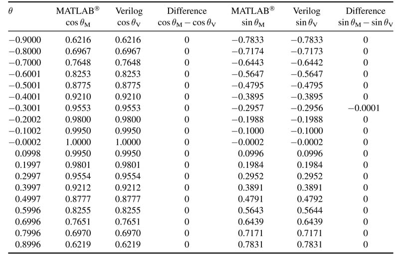
Figure 12.12 Folded CORDIC architecture. (a) Folding factor of 16. (b) Folding factor of 8
MATLAB® and Verilog, respectively, the third column shows the difference in the results. Similarly the last three columns are the same set of values for sin θ.
12.4.4 Time-shared Architecture
The CORDIC algorithm is very regular and a folded architecture can be easily crafted. Depending on the number of cycles available for computing the sine and cosine values, the CORDIC algorithm can be folded by any folding factor. For N =16, the architecture in Figure 12.12(a) is folded by a folding factor of 16. Similarly Figure 12.13(b) shows a folded architecture by folding factor of 8. The valid signal is asserted after the design computes the N iterations. The RTL Verilog for a folding factor of 16 is given here:
module CORDIC_Shared #(parameter M=22, N = 16, LOGN = 4, K=22’h0DBD96)
// InQ2.20 format, value of K = 0.8588 K=22’h0DBD96)
(
input signed [N - 1:0] theta_d,
input clk,
input rst_n,
output reg signed [M-1:0] cos_theta,
output reg signed [M-1:0] sin_theta);
reg signed [M-1:0] x_reg;
regsigned [M-1:0] y_reg;
reg signed [N-1:0] theta_reg;
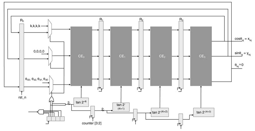
Figure 12.13 Four-slow folded architecture by a folding factor of 4
reg signed [M - 1:0] x_o;
reg signed [M - 1:0] y_o;
reg signed [M-1:0] x_i;
reg signed [M-1:0] y_i;
reg signed [N-1:0] theta_i, theta_o;
reg signed [N-1:0] arcTan;
reg [LOGN-1:0] counter;
reg sel, valid;
integer i;
// Arctan table: radian values are represented in Q1.15 format
always@*
begin
case (counter)
 4’b0000: arcTan = 16’h3B59;
 4’b0001: arcTan = 16’h1F5B;
 4’b0010: arcTan = 16’h0FEB;
 4’b0011: arcTan = 16’h07FD;
 4’b0100: arcTan = 16’h0400;
 4’b0101: arcTan = 16’h0200;
 4’b0110: arcTan = 16’h0100;
 4’b0111: arcTan = 16’h0080;
 4’b1000: arcTan = 16’h0040;
 4’b1001: arcTan = 16’h0020;
 4’b1010: arcTan = 16’h0010;
 4’b1011: arcTan = 16’h0008;
 4’b1100: arcTan = 16’h0004;
 4’b1101: arcTan = 16’h0002;
 4’b1110: arcTan = 16’h0001;
 4’b1111: arcTan = 16’h0000;
 endcase
end
always@*
begin
 sel = |counter;
 valid = &counter;
 if(sel)
 begin
 x_i = x_reg;
 y_i = y_reg;
 theta_i = theta_reg;
 end
 else
 begin
 x_i = K;
 y_i = 0;
 theta_i = theta_d;
 end
 CE_task(x_i, y_i, theta_i, arcTan, counter
 + 1, x_o, y_o, theta_o);
end
always@(posedge clk)
 begin
 if(!rst_n)
 begin
 x_reg <= 0;
 y_reg <= 0;
 theta_reg <= 0;
 counter <= 0;
 end
else if (!valid)
 begin
 x_reg <= x_o;
 y_reg <= y_o;
 theta_reg <= theta_o;
 counter <= counter + 1;
 end
else
 begin
 cos_theta <= x_o;
 sin_theta <= y_o;
end
endmodule
module stimulus;
parameter M = 22;
parameter N = 16;
reg signed [N - 1:0] theta_d;
reg clk;
reg rst_n;
wire signed [M - 1:0] x_o;
wire signed [M - 1:0] y_o;
integer i;
CORDIC_Shared CordicShared(
 theta_d,
 clk,
 rst_n,
 x_o,
 y_o);
initial
begin
 clk = 1; rst_n = 0;theta_d = 0;
 #10
 rst_n = 1;
 theta_d = -29491;
 // For theta_d = -0.9:0.1:0.9
 for (i=0; i<20; i=i+1)
begin
 rst_n = 0;
 #2 rst_n = 1;
 #400
 theta_d = theta_d + 3276;
 end
 #10000
 $finish;
end
always
 #10 clk = ~clk;
initial
$monitor($time, " theta = %d, cos_theta = %d, sine_theta = %d,
 reset = %d", theta_d, x_o, y_o, rst_n);
endmodule
The recursive nature of the time-shared architecture poses a major limitation in folding the architecture at higher degrees as it increases the critical path of the design. The datapath needs to be pipelined but the registers cannot be added straight away. The look-ahead transformation of Chapter 7 can also not be directly applied as the decision logic of computing σi in every stage of the algorithm restricts application of this transform.
12.4.5 C-slowed Time-shared Architecture
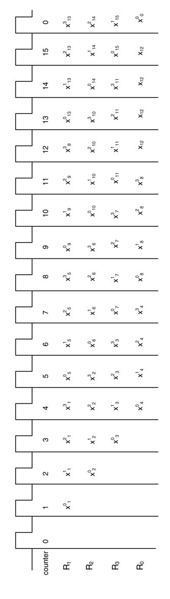
The time-shared architecture in its present configuration cannot be pipelined and can only be C-slowed. The technique to C-slow a design for running multiple threads or instances of input sequences is discussed in detail in Chapter 7. The feedback register is replicated C times and then these registers are retimed to reduce the critical path. This enables the user to initiate C computations of the algorithm in parallel in the time-shared architecture. Each iteration takes N cycles, but the design computes C values in these cycles. A design for N=16 and C=4 is shown in Figure 12.13.
A simple counter-based controller is used to appropriately select the input to each CEi. Two MSBs of the counter are used as select line to three multiplexers. In the first four cycles, four desired angles and associated values of x0 and y0 are input to CE0. All subsequent cycles feed the values from CE3 to R0 to CE0. The successive working of the algorithm for the initial few cycles is elaborated in the timing diagram of Figure 12.14.
The architecture works in lock step calculating N iterations for every input angle, and produces cos θdi and sin θdi for i = 0,…, 3 in four consecutive cycles after the 16th cycle.
12.4.6 Modified CORDIC Algorithm
An algorithm selected for functional simulation in software often poses serious a limitation in achieving HW-specific design objectives. The basic CORDIC algorithm described in Section 12.4.1 is a good example of this limitation. The designer in these cases should explore other HW affine algorithmic options for implementing the same functionality. For the CORDIC algorithm, a modified version is an option of choice that eliminates limitations in exploring parallel and time-shared architecture.
The CORDIC algorithm of Section 12.4.1 requires computation of σi and only then it conditionally adds or subtracts one of the operands while implementing (12.14). This conditional logic restricts the HW design to exploit inherent parallelism in the algorithm. A simple modification can eliminate this restriction and efficient parallel architectures can be realized.
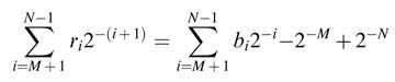
The standard CORDIC algorithm assumes θ as a summation of N positive or negative micro-rotations of angles Δ θi as given by (12.14). A binary representation of a positive value of θ as below can also be considered for micro rotations:
where each term in the summation requires either a positive rotation equal to 2–i or no rotation, depending on the value of the bit bi at location i. This representation cannot be directly used in HW as the constant k of (12.13) becomes data dependent. A modification in the binary representation of θ of (12.15) is thus required that makes values of k data independent.
This independence can be accomplished by recoding the expression in (12.15) to only use + 1 or – 1. This recoding of the binary representation is explained next.
12.4.7 Recoding of Binary Representation as ±1
An N -bit unsigned number b in Q1.(N -1) format can be represented as:
The bits bi in the expression can be recoded to ri ∈ {+1, –1} as:
Figure 12.14 Timing diagram of 4-slow folded CORDIC architecture of Figure 12.13
The MATLAB® code that implements the recoding logic is given here:
 theta_d =1.394;
 % An example value for demonstration of the equivalence
 theta = theta_d;
 N = 16;
 theta = fix(theta * 2^(N-1));
 % Convert theta to Q1.15 format
 % Seperating bits of theta as b=b[1],b[2],….,b[N]
 for i=1:N
 b(N+1-i) =rem(theta, 2);
 theta = fix(theta/2);
 end
 % Recoding 0, 1 bits of bas-1,+1 of r respectively for
 i=1:N
 r(i) =2*b(i) - 1;
 end
 % Computing value of theta using b
 Kb = 0;
 for i = 1:N
 Kb = Kb + b(i)*2^(-(i-1));
 end
 % Computing value of theta using r
 Kr=0;
 for i = 1:N
 Kr = Kr +r(i)*2^(-(i));
 end
 % The constant part
 Kr = Kr + (2^0) - 2^(-N);
 % The three values are the same
 [Kr Kb theta_d]
This recoding requires first giving an initial fixed rotation θinit to cater for the constant factor (20–2–N) along with computing constant K as is done in the basic CORDIC algorithm. The recoding of bi s as ±1 helps in formulating K as a constant and is equal to:
The rotation for θinit can then be first applied, where:
Now to cater for the recoding part, the problem is reformulating to compute the following set of iterations for i=1, …, N–1:
where, unlike σi , the values of ri are predetermined, and these iterations do not include any computations of the Δθi as are done in the basic CORDIC algorithm.
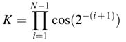
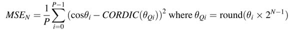
 clear all
 close all
 N=16;
 % Computing the constant value K, the recording part
 K = 1;
 for i = 0:N—1
 K = K* cos(2^(-(i + 1)));
 end
 % The constant initial rotation
 theta_init = (2)^0 - (2)^(-N);
 x0 = K*cos(theta_init);
 y0 = K*sin(theta_init);
 cosine = [];
 sine = [];
 for theta = 0:.1:pi/2
 angle =[0:.1:pi/2];
 theta = round(theta * 2^(N-1));
 % convert theta in Q1.15 format
 % Separating bits of theta as b=b[1],b[2],….,b[N] for k=1:N
 b(N+1-k) = rem(theta, 2);
 theta = fix(theta/2);
 end
 % Recoding shiftedbits of b as r with +1,-1
 for k=1:N
 r(k) = 2*b(k) - 1;
 end
 % First modified CORDIC rotation
 x(1) =x0-r(1)*(tan(2^(-1)) *y0);
 y(1) =y0+r(1)*(tan(2^(-1)) *x0);
 % Remainder of the modified CORDIC rotations
 for k=2:N,
 x(k) = x(k-1) -r(k)*tan(2^(-k)) *y(k-1);
 y(k) = y(k-1) +r(k) * tan(2^(-k)) * x(k-1);
 end
 cosine = [cosine x(k)];
 sine = [sine y(k)];
 end
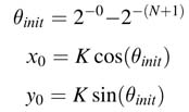
Figure 12.15 Results using CORDIC and modified CORDIC algorithms
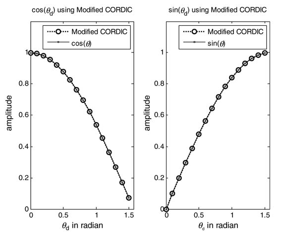
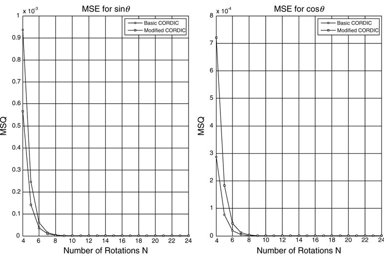
Figure 12.15 shows the results of using CORDIC and modified CORDIC algorithms. A mean squared error (MSE) comparison of the two algorithms for different numbers of rotations N is given in Figure 12.16. The error is calculated for P sets of computation by computing the mean squared difference between the value cos θi in double-precision arithmetic and the value using the CORDIC algorithm for the quantizing value of θi as θ qi in Q1. (N—1) format. The expression for MSE while considering θi as an N -bit number in Q1.(N — 1) format is:
It is clear from the two plots that, for N > 10, mean squared error for both the algorithm is very small, so N= 16 is a good choice for the CORDIC algorithms.
12.5 Hardware Mapping of Modified CORDIC Algorithm
12.5.1 Introduction
One issue in a modified CORDIC algorithm is eliminating tan2–i from (12.17) as it requires multiplication in every stage. This multiplication can be avoided for stages for i > 4 as the values of tan 2–i can be approximated as:
Figure 12.16 Mean square error comparison of CORDIC and modified CORDIC algorithms
This leaves us to pre-compute all possible values of the initial four iterations and store them in a ROM. The MATLAB® code for generating this ROM input is given here:
 tableX=[];
 tableY=[];
 N = 16;
 K = 1;
 for i = 1:N
 K = K* cos(2^(-(i)));
 end
 % The constant initial rotation
 theta_init = (2)^0 - (2)^(-N);
 x0 = K*cos(theta_init);
 y0 = K*sin(theta_init);
 cosine = [];
 sine = [];
 M = 4;
 for index = 0:2^M-1
 for k=1:M
 b(M+1-k) = rem(index, 2);
 index = fix(index/2);
 end
 % Recoding b as r with +1,-1 for k=1:M
 r(k) = 2*b(k) - 1; end
 % First modified CORDIC rotation
 x(1) = x0 - r(1)*(tan(2^(-1)) * y0);
 y(1) = y0 + r(1)*(tan(2^(-1)) * x0);
 % Remainder of the modified CORDIC rotations for k=2:M,
 x(k) = x(k-1) - r(k)* tan(2^(-k)) * y(k-1);
 y(k) = y(k-1) + r(k) * tan(2^(-k)) * x(k-1);
 end
 tableX = [tableX x(M)];
 tableY = [tableY y(M)];
 end
In hardware implementation, the initial M iterations of the algorithm are skipped and the output value from the M th iteration is directly indexed from the ROM. The address for indexing the ROM is calculated using the M most significant bits of b as:
Reading from the ROM directly gives x [M – 1] and y[M – 1] values. The rest of the values of x [k ] and y [k ] are then generated by using the approximation of (12.18). This substitution replaces multiplication by tan 2–iwith a shift by 2–i operation. The equations implementing simplified iterations for i =M + 1, M + 2,…, N are:
Fixed-point implementation of the modified CORDIC algorithm that uses tables for directly indexing the value for the M th iteration and implements (12.20) for the rest of the iterations is given here:
 P = 22;
 N = 16;
 M = 4;
 % Tables are computed for P=22, M=4 and values are in Q2.20 format
 tableX = [
 1045848
 1029530
 997147
 949203
 886447
 809859
 720633
 620162
 510013
 391906
 267683
 139283
 8710
 -122000
 -250805
 -375697];
tableY = [
 65435
 195315
 322148
 443953
 558831
 664988
 760769
 844678
 915406
 971849
 1013127
 1038596
 1047857
 1040767
 1017437
 978229];
 cosine = [];
 sine = [];
 for theta = 0:.01:pi/2
 angle =[0:.01:pi/2];
 theta = round(theta *2^(N-1));
 % convert theta in Q1.N—1 format
 % Seperating bits of theta as b=b[1],b[2],….,b[N]
 for k=1:N
 b(N+1-k) = rem(theta, 2);
 theta = fix(theta/2);
 end
 % Compute index for M = 4;
 index = b(1)*2^3 + b(2)*2^2 + b(3)*2^1 + b(4)*2^0+1;
 x(4)=tableX(index);
 y(4)=tableY(index);
 % Recoding b[M+1], b[M+2],…, b[n] asr with +1,-1 for k=M+1:N
 r(k) =2*b(k) - 1;
 end
 % Simplified iterations for modified CORDIC rotations
 for k=M+1:N,
 x(k) = x(k-1) -r(k)*2^(-k) * y(k-1);
 y(k) = y(k-1) +r(k) *2^(-k) * x(k-1);
 end
 % For plotting, convert the values of x and y to
 floating point format
 cosine= [cosinex(k)/(2^(P-2))];
 sine= [sine y(k)/(2^(P-2))];
 end
This modification results in simple fully parallel and time-shared HW implementations. The fully parallel architecture is shown in Figure 12.17. The architecture can also be easily pipelined.
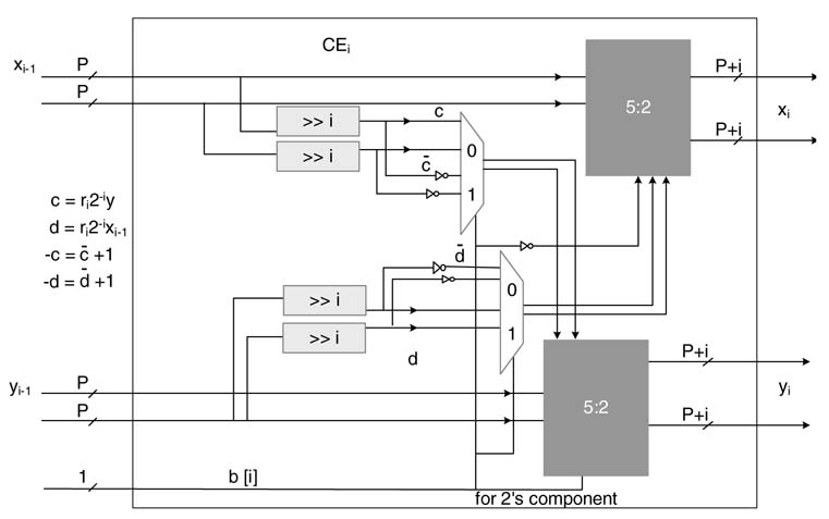
These iterations can also be merged together to be reduced using a compression tree for effective HW mapping [9]. A merged cell that takes partial-sum and partial-carry results from state (i—1) and then generates partial results for iteration i while using a5:2 compression tree is shown in Figure 12.18.
For the time-shared architecture, multiple CEs can be used to fold the architecture for any desired folding factor.
12.5.2 Hardware Optimization
In many applications the designer may wish to explore optimization above what is apparently perceived from the algorithm. There is no established technique that can be generally used, but a deep analysis of the algorithm often reveals novel ways of optimization. This section demonstrates this assertion by presenting a novel algorithm that computes the sine and cosine values in a single stage, thus enabling zero latency with very low area and power consumption [10].
Consider a fixed-point implementation of the modified CORDIC algorithm. As the iterations now do not depend on values of Δθi, the values of previous iterations can be directly substituted into the current iteration. If we consider M=4, then indexing into the tables gives the values of x4 and y4. Now these values are used to compute the iteration for i = 5 as:
The iteration for i = 6 calculates:
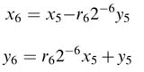
Now substituting expressions for x5 and y5 from (12.21) in the above expressions, we get:
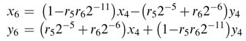
Figure 12.17 FDA of modified CORDIC algorithm
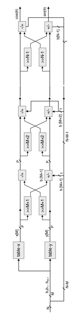
Figure 12.18 A CE with compression tree
Adopting the same procedure – that is, first writing expressions for x7 and y7 and then substituting values of x6 and y6 – we get:

It is evident from the above expressions that the terms with 2–x with x > P will shift the entire value outside the range of the required precision and thus can simply be ignored. If all these terms are ignored and we substitute previous expressions into the current iteration, we get the final iteration as a function of x4 and y4. The final expressions for P = 16 are:
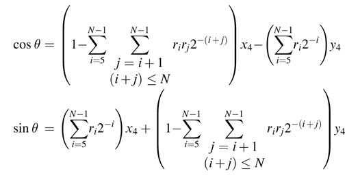
Each term in a bracket is reduced to one term. For P =16, the first term in the bracket results in 12 terms and the second bracket also contains 12 terms. These expressions can be implemented as two compression trees. All the iterations of the CORDIC algorithm are merged into one expression and the expression can be effectively computed in a single cycle.
The MATLAB® code for the algorithm is given below. This uses the same table as generated in MATLAB® code earlier for computing values of x4 and y4:
 cosine = [];
 sine = [];
 N = 16;
 P = 16;
 M = 4;
 for theta =.00:.05:pi/2
 angle =[0.00:.05:pi/2];
 theta = round(theta * 2^(N-1));
 % convert theta in Q1.N format
 % Separating bits of theta as b=b[1],b[2],….,b[N]
 for k=1:N
 b(N+1-k) = rem(theta, 2);
 theta = fix(theta/2);
 end
 % Compute index for M = 4;
 index = b(1)*2^3 + b(2)*2^2 + b(3)*2^1 + b(4)*2^0+1;
 x4=tableX(index);
 y4=tableY(index);
 % Recoding b[M+1], b[M+2],…, b[n] asr with +1,-1
 for k=M+1:N
 r(k) = 2*b(k) - 1;
 end
 xK = (1-r(5)*r(6)*2^(-11) -r(5)*r(7)*2^(-12) -r(5)*r(8)*2^(-13) -r(5)*r(9)*2^(-14) -r(5)*r(10)*2^(-15) -r(5)*r(11)*2^(-16)… -r(6)*r(7)*2^(-13) -r(6)*r(8)*2^(-14)-r(6)*r(9)*2^(-15) -r(6)*r(10)*2^(-16)… -r(7)*r(8)*2^(-15) -r(7)*r(9)*2^(-16)*x4 - (r(5)*2^(-5)+r(6)*2^(-6) +r(7)*2^(-7)+r(8)*2^(-8)+r(9)*2^(-9)+r(10)*2^ (-10)… +r(11)*2^(-11)+r(12)*2^(-12)+r(13)*2^(-13) +r(14)*2^(-14)+r(15)*2^(-15)+r(16)*2^(-16))*y4;
 yK = (r(5)*2^(-5)+r(6)*2^(-6)+r(7)*2^(-7) +r(8)*2^(-8)+r(9)*2^(-9) +r(10)*2^(-10)… +r(11)*2^(-11)+r(12)*2^(-12) +r(13)*2^(-13)+r(14)*2^(-14)+r(15)*2^(-15) +r(16)*2^(-16))*x4+… (1-r(5)*r(6)*2^(-11) -r(5)*r(7)*2^(-12) -r(5)*r(8)*2^(-13) -r(5)*r(9)*2^(-14) -r(5)*r(10)*2^(-15) -r(5)*r(11)*2^(-16)… -r(6)*r(7)*2^(-13) -r(6)*r(8)*2^(-14)-r(6)*r(9)*2^(-15) -r(6)*r(10)*2^(-16)… -r(7)*r(8)*2^(-15) -r(7)*r(9)*2^(-16))*y4;
 % For plotting, convert the values of x and y to floating point format,
 % using the original format used for table generation where P=22
 cosine = [cosine xK/(2^(20))];
 sine = [sine yK/(2^(20))];
 end
12.5.3 Novel Optimal Hardware Design
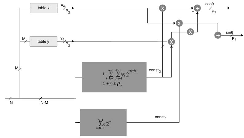
Yet another approach to designing optimal hardware of the CORDIC is to map the expressions in ri into two binary constants using reverse encoding and then use four multipliers and two adders to compute the desired results. This novel technique results in a single-stage CORDIC architecture. The design is shown in Figure 12.19.
The inverse coding is accomplished using (12.16). The inverse coding for const1 issimply derived as:
In HW design, as the original bi are kept intact they are used for computing the two constants. To cater for the 2–N term in (12.22), a 1 is appended to b as the LSB bN, and for the –2–M factor the corresponding bM+1 bit is flipped and is assigned a negative weight. Then const1 is given as:
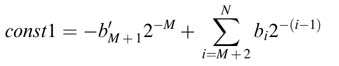
where b'M+1 is the complement of bit bM+1. Similarly for const2, the first rk are computed for i =M+1,…, N — 1 as:
These rrk are then inverse coded using (12.22) and an equivalent value is computed similar to the const1 computation by expression in (12.23). For N = 16 and P = 16, this requires computing the
Figure 12.19 Optimal hardware design with single-stage implementation of the CORDIC algorithm
values of rrk for three values of i . First for i = 5, rrk are computed and inverse coded as a constant value:
These t5;j are reverse-coded as b′ks as:
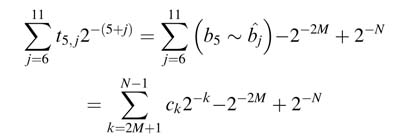
where ck=b5~![]() j for j=6,7,….,11 where k=5 +j
j for j=6,7,….,11 where k=5 +j
Using tk after catering for the two terms –2–2Mand2–N, the value of the constant beta is computed as:
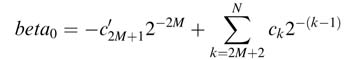
Following the same steps, values of bet a1 and beta2 are computed for i = 6 and i = 7, respectively. The details of the computation are given here in MATLAB® code:
 clear all
 close all
 % Values for first four iterations in Q2.16 format
 table=[65366 4090
 64346 12207
 62322 20134
 59325 27747
 55403 34927
 50616 41562
 45040 47548
 38760 52792
 31876 57213
 24494 60741
 16730 63320
 8705 64912
 544 65491
 -7625 65048
 -15675 63590
 -23481 61139];
 N = 16;
 P = 18; % 18-bit width for catering for truncation effects
 M = 4;
 cosSSC = []; sinSSC = []; % arrays of single stage cordic
 cosQ = []; sinQ = []; % arrays for 16-bit fixed point precision
 cosD = []; sinD = []; % arrays for double precision floating point values
 for theta_f =.0:.001:pi/2
 % convert theta in Q1.5 format
 theta = round(theta_f * 2^(N-1)); % 16-bit fixed-point value of theta
 thetaQ = theta/2^(N-1); % 16-bit quantized theta in floating point format
 % separating bits of theta as
 % b=b[1],b[2],….,b[N]
 for k=1:N
 b(N+1-k) = rem(theta, 2); theta = fix(theta/2);
 end
 %compute index for M = 4;
 index=b(1)*2^3 + b(2)*2^2 + b(3)*2^1 + b(4)+1;
 x4 = table(index,1); y4 = table(index,2);
 % recoding b[M+1],b[M+2],…,b[n] as r-> +1,-1
 for k=5:N
 r(k) = 2*b(k) - 1;
 end
 % computing const2 for all values of i and j
 % i+j<=P
 sum = 0;
 for i=5:7;
 for j=i+1:P-i
 k = i+j;
 sum = sum + r(i)*r(j)*2^(-k);
 end
 end
 const2 = 1 - sum; const1 = 0;
 for k=M+1:N
 const1= const1+r(k)*2^(-(k));
 end
 % single stage modified CORDIC butterfly
 xK = const2 * x4 - const1 * y4;
 yK = const1 * x4 + const2 * y4;
 % arrays for recording single state, quantized and double precision
 % results for final comparision
 cosSSC = [cosSSC xK]; sinSSC = [sinSSC yK];
 cosD = [cosD cos(thetaQ)]; sinD = [sinD sin(thetaQ)];
 cosQ = [cosQ (round(cos(thetaQ)*2^14)/2^14)]; sinQ = [sinQ
 (round(sin(thetaQ)*2^14)/2^14)];
 end
 % computing mean square errors, Single Stage CORDIC performs better
 MSEcosQ = mean((cosQ-cosD).^2); % MSEcosQ = 3.0942e-010
 MSEcosSSC = mean((cosSSC./2^16-cosD).^2) % MSEcosSSC = 1.3242e-010
 MSEsinQ = mean((sinQ-sinD).^2); % MSEsinQ = 3.1869e-010
 MSEsinSSC = mean((sinSSC./2^16-sinD).^2); % MSEsinSSC = 1.2393e-010
 MSEcosQ MSEcosSSC]
 MSEsinQ MSEsinSSC]
The code is mapped in hardware for optimal implementation of the CORDIC algorithm. Verilog code of the design is given here (the code can be further optimized by using a compression tree for computing const 2):
 module CORDIC_Merged #(parameter M = 4, N = 16, P1 = 18)
 // Q2.16 format values of x4 and y4 are stored in the ROM)
 (
 input [N-1:0] bin,
 // value of theta_d in Q1.N-1 format
 // input clk,
 output reg signed [P1 - 1:0] cos_theta,
 output reg signed [P1 - 1:0] sin_theta);
 reg [N-1:0] b;
 reg signed [P1-1:0] x4;
 reg signed [P1-1:0] y4;
 reg signed [P1-1:0] beta0, beta1, beta2;
 reg signed [P1-1:0] const1, const2;
 reg signed [2*P1-1:0] mpy0, mpy1, mpy2, mpy3;
 reg signed [P1-1:0] xK, yK;
 wire [5:0] c0;
 wire [3:0] c1;
 wire [1:0] c2;
 reg [M-1:0] index;
 // table to store all possible values of x4 and y4 in Q2.16 format
 always@*
 begin
 case (index)
 4’b0000: begin x4 = 65366; y4 = 4090; end
 4’b0001: begin x4 = 64346; y4 = 12207; end
 4’b0010: begin x4 = 62322; y4 = 20134; end
 4’b0011: begin x4 = 59325; y4 = 27747; end
 4’b0100: begin x4 = 55403; y4 = 34927; end
 4’b0101: begin x4 = 50616; y4 = 41562; end
 4’b0110: begin x4 = 45040; y4 = 47548; end
 4’b0111: begin x4 = 38760; y4 = 52792; end
 4’b1000: begin x4 = 31876; y4 = 57213; end
 4’b1001: begin x4 = 24494; y4 = 60741; end
 4’b1010: begin x4 = 16730; y4 = 63320; end
 4’b1011: begin x4 = 8705; y4 = 64912; end
 4’b1100: begin x4 = 544; y4 = 65491; end
 4’b1101: begin x4 = -7625; y4 = 65048; end
 4’b1110: begin x4 = -15675; y4 = 63590; end
 4’b1111: begin x4 = -23481; y4 = 61139; end
 endcase
 end
 // the NOVALITY, computing the values of constants for single
 // stage CORDIC
 assign c0 = {6{b[5]}}~^b[11:6];
 assign c1 = {4{b[6]}}~^b[10:7];
 assign c2 = {2{b[7]}}~^b[9:8];
 always@*
 begin
 index = b[15:12];
 beta0 = {{12{~c0[5]}},c0[4:0],1’b1};
 beta1 = {{14{(~c1[3])}},c1[2:0],1’b1};
 beta2 = {{16{~c2[1]}},c2[0], 1’b1};
 const2 = {1’b0,16’h8000,1’b0} - (beta0 + beta1 + beta2);
 const1 = {{6{~b[11]}},b[10:0],1’b1};
 end
 always@*
 begin
 mpy0 = const2 * x4;
 mpy1 = const1 * y4;
 xK = mpy0[34:16] - mpy1[34:16];
 mpy2 = const1 * x4;
 mpy3 = const2 * y4;
 yK = mpy2[34:16] + mpy3[34:16];
 end
 always @*
 // replace by sequential block with clock for sythesis timing
 begin
 b = bin;
 cos_theta = xK;
 sin_theta = yK;
 end
 endmodule
 //
 module stimulus;
 parameter P = 18;
 parameter N = 16;
 reg signed [N - 1:0] theta_d;
 wire signed [P - 1:0] x_o;
 wire signed [P - 1:0] y_o;
 integer i;
 integer outFile;
 CORDIC_Merged merged (
 theta_d,
 x_o,
 y_o);
 initial
 outFile = $fopen("monitor_merge.txt","w");
 always@ (x_o, y_o)
 $fwrite(outFile, " %d %d
", x_o, y_o);
 initial
 begin
 #5 theta_d = 0;
 for (i=0; i<16; i=i+1)
 #20 theta_d = theta_d + 3276;
 #400 $fclose(outFile);
 $finish;
 end
 initial
 $monitor($time, " theta=%d, cos_theta=%d, sine_theta=%d
", theta_d, x_o,
 y_o); endmodule
Figure 12.20 Schematic of single-stage CORDIC design
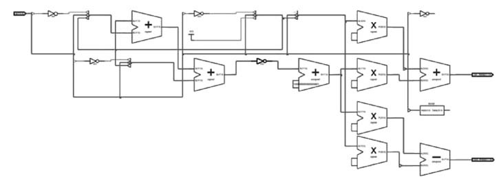
The code is synthesized using Xilinx ISE 10.1 on a Vertix-2 device. The design computes values of sin θ and cos θ in a single stage and single cycle. The design can also be easily pipelined for highspeed operation.
The RTL schematic of the synthesized code is given in Figure 12.20. The schematic clearly shows the logic for computing the constants, a ROM for table look-up, four multipliers and an adder and a subtractor for computing the single-stage CORDIC.
Exercises
Exercise 12.1
Pipeline the modified CORDIC algorithm and implement the design in RTL Verilog. Assume θ is a 16-bit precision number and keep the internal datapath of the CORDIC to be 22 bits wide. Pipeline the design at every CE level.
Exercise 12.2
Design a folded architecture for a modified CORDIC algorithm with folding factors of 16, 8 and 4. Assume θ is a 16-bit precision number and keep the internal datapath of the CORDIC to be 16 bits wide.
Exercise 12.3
Design a 4-slow architecture for the folded modified CORDIC algorithm with folding factor of 4. Implement the design in RTL Verilog. Assume θ is a 12-bit precision number and keep the internal datapath of the CORDIC to be 14 bits wide.
Exercise 12.4
The modified CORDIC algorithm can be easily mapped in bit-serial and digital-serial designs. Design a bit-serial architecture for 16-bit precision of angle θ . Keep the internal datapath to be 16 bits wide. Modify the design to take 4-bit digits.
Exercise 12.5
Use a compression tree to compute const 2 of the novel CORDIC algorithm of Section 12.5.3. Rewrite RTL code and synthesize the design. Compare the design with the one given in the section for any improvement in area and timing.
References
1. J. Valls, T. Sansaloni, A. P. Pascual, V. Torres and V. Almenar, “The use of CORDIC in software defined radios: a tutorial,” IEEE Communications Magazine , 2006, vol. 44, no. 9, pp. 46–50.
2. K. Murota, K. Kinoshita and K. Hirade, “GMSK modulation for digital mobile telephony,” IEEE TransactionsonCommunications , 1981, vol. 29, pp. 1044–1050.
3. J. Volder, “The CORDIC computingtechnique ,” IRE TransactionsonComputing , 1959, pp. 330–334.
4. J. S. Walther, “A unified algorithm for elementary functions,” in ProceedingsofAFIPSSpringJointComputer Conference , 1971, pp. 379–385.
5. S. Wang, V. Piuri and E. E. Swartzlander, “Hybrid CORDIC algorithms,” IEEETransactionsonComputing , 1997, vol. 46, pp. 1202–1207.
6. D. De Caro, N. Petra and G. M. Strollo, “A 380-MHz direct digital synthesizer/mixer with hybrid CORDIC architecture in 0.25-micron CMOS,” IEEE Journal of Solid-State Circuits , 2007, vol. 42, pp. 151–160.
7. T. Rodrigues and J. E. Swartzlander, “Adaptive CORDIC: using parallel angle recoding to accelerate rotations,” IEEE Transactions on Computers , 2010, vol. 59, pp. 522–531.
8. P. K. Meher, J. Valls, T.-B. Juang, K. Sridharan and K. Maharatna, “50 years of CORDIC: algorithms, architectures, and applications,” IEEE Transactions on Circuits and Systems I, 2009, vol. 56, pp. 1893–1907.
9. T. Zaidi, Q. Chaudry and S. A. Khan, “An area- and time-efficient collapsed modified CORDIC DDFS architecture for high-rate digital receivers ,”in Proceedings of INMIC , 2004, pp. 677–681.S.A.Khan, ‘‘A fixed-point single stage CORDIC architecture’’, Technical report CASE, June 2010.