
3
System Design Flow and Fixed-point Arithmetic
Pure mathematics is, in its way, the poetry of logical ideas.
3.1 Overview
This chapter describes a typical design cycle in the implementation of a signal processing application. The first step in the cycle is to capture the requirements and specifications (R&S) of the system. The R&S usually specify the sampling rate, a quantitative measure of the system’s performance, and other application-specific parameters. The R&S constrain the designer to explore different design options and algorithms to meet them in the most economical manner. The algorithm exploration is usually facilitated by MATLAB®, which is rich in toolsets, libraries and functions. After implementation and analysis of the algorithm in MATLAB®, usually the code is translated into higher level programming languages, for example, C/C ++ or C#.
This requires the chapter to focus on numbering systems. Representing signed numbers in two’s complement format is explained. In this representation, the most significant bit (MSB) has negative weight and the remainder of the bits carry positive weights. Although the two’s complement arithmetic greatly helps addition and subtraction, as subtraction can be achieved by addition, the negative weight of the sign bit influences multiplication and shifting operations. As the MSB of a signed number carries negative weight, the multiplication operation requires different handling for different types of operand. There are four possible combinations for multiplication of two numbers: unsigned-unsigned, signed-unsigned, unsigned-signed and signed-signed. The chapter describes two’s complement multiplication to highlight these differences. Scaling of signed number is described as it is often needed while implementing algorithms in fixed-point format.
Characteristics of two’s complement arithmetic from the hardware (HW) perspective are listed with special emphasis on corner cases. The designer needs to add additional logic to check the corner cases and deal with them if they occur. The chapter then explains floating-point format and builds the rationale of using an alternate fixed-point format for DSP system implementation. The chapter also justifies this preference in spite of apparent complexities and precision penalties. Cost, performance and power dissipation are the main reasons for preferring fixed-point processors and HW for signal processing systems. The fixed-point implementations are widely used for signal processing systems whereas floating-point processors are mainly used in feedback control systems where precision is of paramount importance. The chapter also highlights that currently integrated high gate counts on FPGAs encourages designers to use floating-point blocks as well for complex DSP designs in hardware.
The chapter then describes the equivalent format used in implementing floating-point algorithms in fixed-point form. This equivalent format is termed the Qn.m format. All the floating-point variables and constants in the algorithm are converted to Qn.m format. In this format, the designer fixes the place of an implied decimal point in an N -bit number such that there are n bits to the left and m bits to the right. All the computations in the algorithm are then performed on fixed-point numbers.
The chapter gives a systematic approach to converting a floating-point algorithm in MATLAB® to its equivalent fixed-point format. The approach involves the steps of levelization, scalarization, and then computation of ranges for specifying the Qn.m format for different variables in the algorithm. The fixed-point MATLAB® code then can easily be implemented. The chapter gives all the rules to be followed while performing Qn.m format arithmetic. It is emphasized that it is the developer’s responsibility to track and manage the decimal point while performing different arithmetic operations. For example, while adding two different Q-format numbers, the alignment of the decimal point is the responsibility of the developer. Similarly, while multiplying two Q-format signed numbers the developer needs to throw away the redundant sign bit. This discussion leads to some critical issues such as overflow, rounding and scaling in implementing fixed-point arithmetic. Bit growth is another consequence of fixed-point arithmetic, which occurs if two different Q-format numbers are added or two Q-format numbers are multiplied. To bring the result back to pre-defined precision, it is rounded and truncated or simply truncated. Scaling or normalization before truncation helps to reduce the quantization noise. The chapter presents a comprehensive account of all these issues with examples.
For communication systems, the noise performance of an algorithm is critical, and the finite precision of numbers also contributes to noise. The performance of fixed-point implementation needs to be tested for different ratios of signal to quantization noise (SQNR). To facilitate partitioning of the algorithm in HW and SW and its subsequent mapping on different components, the chapter describes algorithm design and coding guidelines for behavioral implementation of the system. The code should be structured such that the algorithm developers, SW designers and HW engineers can correlate different implementations and can seamlessly integrate, test and verify the design and can also fall back to the original algorithm implementation if there is any disagreement in results and performance. FPGA vendors like Xilinx and Altera in collaboration with Mathworks are also providing Verilog code generation support in several Simulink blocks. DSPbuilder from Altera [1] and System Generator from Xilinx [2] are excellent utilities. In a Simulink environment these blocksets are used for model building and simulation. These blocks can then be translated for HW synthesis. A model incorporating these blocks also enables SW/HW co-simulation. This co-simulation environment guarantees bit and cycle exactness between simulation and HW implementation. MATLAB® also provides connectivity with ModelSim though a Link to ModelSim utility.
Logic and arithmetic shifts of numbers are discussed. It is explained that a full analysis should be performed while converting a recursive digital system to fixed-point format. Different computational structures exist for implementing a recursive system. The designer should select a structure that is least susceptible to quantization noise. The MATLAB® filter design toolbox is handy to do the requisite analysis and design space exploration. The chapter explains this issue with the help of an example. The chapter ends by giving examples of floating-point C code and its equivalent fixed-point C conversion to clarify the differences between the two implementations.
To explain different topics in the chapter several numerical examples are given. These examples use numbers in binary, decimal and hexadecimal formats. To remove any confusion among these representations, we use different ways of distinguishing the formats. A binary number is written with a base 2 or b, such as 1001b and 1002. The binary numbers are also represented in Verilog format, for example 3'b 1001. Decimal numbers are written without any base or with a base 10, like –0.678 and –0.67810. The hexadecimal representation is 0×23df.
3.2 System Design Flow
3.2.1 Principles
This section looks at the design flow for an embedded system implementing a digital signal processing application. Such a system in general consists of hybrid target technologies. In Chapter 1 the composition of a representative system is discussed in detail. While designing such an embedded system, the application is partitioned into hardware and software components.
Figure 3.1 depicts the design flow for an embedded signal processing application. Capturing R&S is the first step in the design cycle. The specifications are usually in terms of requirements on the sampling rate, a quantitative measure of performance in the presence of noise, and other application-specific parameters. For example, for a communication system a few critical requirements are: maximum supported data rate in bits per second (bps) at the transmitter, the permissible bit error rate (BER), the channel bandwidth, the carrier and intermediate frequencies, the physical form factor, power rating, user interfaces, and so on. The R&S summary helps the designer to explore different design options and flavors of algorithms.
Figure 3.1 System-level design components
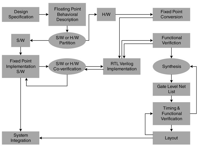
The requirements related to digital design are forwarded to algorithm developers. The algorithm developers take these requirements and explore digital communication techniques that can meet the listed specifications. These algorithms are usually coded in behavioral modeling tools with rich predesigned libraries of functions and graphical aids. MATLAB® has become the tool of choice for algorithm development and exploration. It is up to an experienced designer to finalize an algorithm based on its ease of implementation and its compliance to the R&S of the design. After the implementation of the algorithm in MATLAB®, usually the code is translated into high level language, for example, C/C++ or C#. Although MATLAB® has been augmented with fixed-point tools and a compiler that can directly convert MATLAB® code to C or C++, but in many instances a hand-coded implementation in C/C++ is preferred for better performance. In many circumstances it is also important for the designer to comprehend the hidden complexities of MATLAB® functions: first to make wise HW/SW partitioning decisions, and then to implement the design on an embedded platform consisting of GPP, DSPs, ASICs and FPGSs.
Partitioning of the application into HW/SW is a critical step. The partitioning is driven by factors like performance, cost, form factor, power dissipation, time to market, and so on. Although an all-software implementation is easiest to code and implement, in many design instances it may not be feasible. Then the designer needs to partition the algorithm written in C/C++ into HW and SW parts. A well-structured, computationally intensive and easily separable code is preferably mapped on hardware, whereas the rest of the application is mapped in software. Both the parts are converted to fixed-point format.
For the SW part a target fixed-point DSP is selected and the designer takes the floating-point code that is meant for SW implementation and converts it to fixed-point format. This requires the designer to convert all the variables and constants earlier designed using double- or single-precision floatingpoint format to standard fixed-point variables of type char, short and int, requiring 8-bit, 16-bit or 32-bit precisions, respectively. Compared with fixed-point conversion for mapping on a DSP, the conversion to fixed-point for HW mapping requires more deliberation because any number of bits can be used for different variables and constants in the code. Each extra bit in HW costs additional resources, and finding the optimal width of all variables requires several iterations with different precisions of variables settings.
After converting the code to the requisite fixed-point format, it is always recommended to simulate both the HW and SW parts and characterize the algorithm for different simulated signal-to-noise ratios. After final partitioning and fixed-point conversion, the HW designer explores different architectures for the implementation. This book presents several effective techniques to be used for design space exploration. The designed architecture is then coded in a hardware description language (HDL), maybe Verilog or VHDL. The designer needs to write test vectors to thoroughly verify the implementation. In instances where part of the application is running in SWon a DSP, it is critical to verify the HW design in a co-verification environment. The designer can use System-Verilog for this purpose. Several commercially available tools like MATLAB® also help the designer to co-simulate and co-verify the design. The verified RTL code is then synthesized on a target technology using a synthesis tool. If the technology is an FPGA, the synthesis tool also generates the final layout. In the case of an ASIC, a gate-level netlist is generated. The designer can perform timing verification and then use tools to lay out the design.
In parallel, a printed circuit board (PCB) is designed. The board, along with all the necessary interfaces like PCI, USB and Ethernet, houses the hybrid technologies such as DSP, GPPs, ASICs and FPGAs. Once the board is ready the first task is to check all the devices on the board and their interconnections. The application is then mapped where the HW part of it runs on ASICs or FPGAs and the SW executes on DSPs and GPPs.
Table 3.1 General requirement specification of a UHF radio
| Characteristics | Specification |
| Output power | 2W |
| Spurious emission | < 60dB |
| Harmonic suppression | > 55dB |
| Frequency stability | 2 ppm or better |
| Reliability | > 10,000 hours MTBF minimum < 30 minutes MTTR |
| Handheld | 12V DC nickel metal hydride, nickel cadmium or lithium-ion (rechargeable) battery pack |
3.2.2 Example: Requirements and Specifications of a UHF Software-defined Radio
Gathering R&S is the first part of the system design. This requires a comprehensive understanding of different stakeholders. The design cycle starts with visualizing different components of the system and then breaking up the system into its main components. In the case of a UHF radio, this amounts to breaking the system down into an analog front end (AFE) and the digital software-defined radio (SDR). The AFE consists of an antenna unit, a power amplifier and one or multiple stages of RF mixer, whereas the digital part of the receiver takes the received signal at intermediate frequency (IF) and its corresponding transmitter part up-converts the baseband signal to IF and passes it to AFE. Table 3.1 lists general requirements on the design. These requirements primarily list the power output, spurious emissions and harmonic suppression outside the band of operation, and the frequency stability of the crystal oscillator in parts per million (ppm). A frequency deviation of 2ppm amounts to 0.0002% over the specified temperature range with respect to the frequency at ambient temperature 25 °C. This part also lists mean time between failure (MTBF) and mean time to recover (MTTR).Table 3.2, lists transmitter and receiver specifications. These are important because the algorithm designer has to explore digital communication techniques to meet them. The specification lists OFDM to be used supporting BPSK, QPSK and QAM modulations. The technique caters for multipath effects and fast fading due to Doppler shifts as the transmitter and receiver are expected to move very fast relative to each other. The communication system also supports different FEC techniques at 512 kbps. Further to this the system needs to fulfill some special requirements. Primarily these are to support frequency hopping and provide flexibility and programmability in the computing platform for mapping additional waveforms. All these specifications pose stringent computational requirements on the digital computing platform and at the same time require them to be programmable; that is, to consist of GPP, DSP and FPGA technologies.
Table 3.2 Transmitter and receiver characteristics
| Characteristic | Specification |
| Frequency range BW | 420MHz to 512MHz |
| Data rate | Up to 512 kbps multi-channel non-line of sight |
| Channel | Multi-path with 15ms delay spread and 220 km/h relative speed between transmitter and receiver |
| Modulation | OFDM supporting BPSK, QPSK and QAM |
| FEC | Turbo codes, convolution, Reed–Solomon |
| Frequency hopping | > 600 hops/s, frequency hopping on full hopping band |
| Waveforms | Radio works as SDR and should be capable of accepting additional waveforms |
The purpose of including this example is not to entangle the reader’s mind in the complexities of a digital communication system. Rather, it highlights that a complete list of specifications is critical upfront before initiating the design cycle of developing a signal processing system.
3.2.3 Coding Guidelines for High-level Behavioral Description
The algorithm designer should always write MATLAB® code for easy translation into C/C++ and its subsequent HW/SW partitioning, where HW is implementation is in RTL Verilog and SW components are mapped on DSP. Behavioral tools like MATLAB® provide a good environment for the algorithm designer to experiment with different algorithms without paying much attention to implementation details. Sometimes this flexibility leads to a design that does not easily go down in the design cycle. It is therefore critical to adhere to the guidelines while developing algorithms in MATLAB®. The code should be written in such a way that eases HW/SW partitioning and fixed-point translation. The HW designer, SW developer and verification engineer should be able to conveniently fall back to the original implementation in case of any disagreement. The following are handy guidelines.
1. The code should be structured in distinct components defined as MATLAB® functions with defined interfaces in terms of input and output arguments and internal data storages. This helps in making meaningful HW/SW partitioning decisions.
2. All variables and constants should be defined and packaged in data structures. All user-defined configurations should preferably be packaged in one structure while system design constants are placed in another structure. The internal states must be clearly defined as structure elements for each block and initialized at the start of simulation.
3. The code must be designed for the processing of data in chunks. The code takes a predefined block of data from an input FIFO (first-in/first-out) and produces a block of data at the output, storing it in an output FIFO, mimicking the actual system where usually data from an analog-to-digital converter is acquired in a FIFO or in a ping-pong buffer and then forwarded to HW units for processing. This is contrary to the normal tendency followed while coding applications in MATLAB®, where the entire data is read from a file for processing in one go. Each MATLAB® function in the application should process data in blocks. This way of processing data requires the storing of intermediate states of the system, and these are used by the function to process the next block of data.
An example MATLAB® code that works on chunks of data for simple baseband modulation is shown below. The top-level module sets the user parameters and calls the initialization functions and main modulation function. The processing is done on a chunk-by-chunk basis.
% BPSK = 1, QPSK = 2, 8PSK = 3, 16QAM = 4
% All-user defined parameters are set in structure USER_PARAMS
USER_PARAMS.MOD_SCH = 2; %select QPSK for current simulation
USER_PARAMS.CHUNK_SZ = 256; %set buffer size for chunk by chunk processing
USER_PARAMS.NO_CHUNKS = 100;% set no of chunks for simulation
% generate raw data for simulation
raw_data = randint(1, USER_PARAMS.NO_CHUNKS*USER_PARAMS.CHUNK_SZ)
% Initialize user defined, system defined parameters and states in respective
% Structures
PARAMS = MOD_Params_Init(USER_PARAMS);
STATES = MOD_States_Init(PARAMS);
mod_out = [];
% Code should be structured to process data on chunk-by-chunk basis
for iter = 0:USER_PARAMS.NO_CHUNKS-1
 in_data = raw_data
 (iter*USER_PARAMS.CHUNK_SZ+1:USER_PARAMS.CHUNK_SZ*(iter+1));
 [out_sig,STATES]= Modulator(in_data,PARAMS,STATES);
 mod_out = [mod_out out_sig];
end
The parameter initialization function sets all the parameters for the modulator.
% Initializing the user defined parameters and system design parameters
% In PARAMS
function PARAMS = MOD_Params_Init(USER_PARAMS)
% Structure for transmitter parameters
PARAMS.MOD_SCH = USER_PARAMS.MOD_SCH;
PARAMS.SPS = 4; % Sample per symbol
% Create a root raised cosine pulse-shaping filter
PARAMS.Nyquist_filter = rcosfir(.5, 5, PARAMS.SPS, 1);
% Bits per symbol, in this case bits per symbols is same as mod scheme
PARAMS.BPS = USER_PARAMS.MOD_SCH;
% Lookup tables for BPSK, QPSK, 8-PSK and 16-QAM using gray coding
BPSK_Table = [(-1 + 0*j) (1 + 0*j)];
QPSK_Table = [(-.707 -.707*j) (-.707 +.707*j)…
 (.707 -.707*j) (.707 +.707*j)];
PSK8_Table = [(1 + 0j) (.7071 +.7071i) (-.7071 +.7071i) (0 + i)…
 (-1 + 0i) (-.7071 -.7071i) (.7071 -.7071i) (0 - 1i)];
QAM_Table = [(-3 + -3*j) (-3 + -1*j) (-3 + 3*j) (-3 + 1*j) (-1 + -3*j)…
 (-1 + -1*j) (-1 + 3*j) (-1 + 1*j) (3 + -3*j) (3 + -1*j)…
 (3 + 3*j) (3 + 1*j) (1 + -3*j) (1 + -1*j) (1 + 3*j) (1 + 1*j)];
% Constellation selection according to bits per symbol
if(PARAMS.BPS == 1)
 PARAMS.const_Table = BPSK_Table;
elseif(PARAMS.BPS == 2)
 PARAMS.const_Table = QPSK_Table;
elseif(PARAMS.BPS == 3)
 PARAMS.const_Table = PSK8_Table;
elseif(PARAMS.BPS == 4)
 PARAMS.const_Table = QAM_Table;
else
 error(ERROR!!! This constellation size not supported)
end
Similarly the state initialization function sets all the states for the modulator for chunk-by-chunk processing of data. For this simple example, the symbols are first zero-padded and then they are passed through a Nyquist filter. The delay line for the filter is initialized in this function. For more complex applications this function may have many more arrays.
function STATES =MOD_States_Init(PARAMS)
% Pulse shaping filter delayline
STATES.filter_delayline = zeros(1,length(PARAMS.Nyquist_filter)-1);
And finally the actual modulation function performs the modulation on a block of data.
function [out_data, STATES] =Modulator(in_data, PARAMS, STATES);
% Bits to symbols conversion

sym = reshape(in_data,PARAMS.BPS,length(in_data)/PARAMS.BPS)’;
% Binary to decimal conversion
sym_decimal = bi2de(sym);
% Bit to symbol mapping
const_sym= PARAMS.const_Table(sym_decimal+1);
% Zero padding for up-sampling
up_sym = upsample(const_sym,PARAMS.SPS);
% Zero padded signal passed through Nyquist filter
[out_data, STATES.filter_delayline] =
 filter(PARAMS.Nyquist_filter,1,up_sym,
 STATES.filter_delayline);
This MATLAB® example defines a good layout for implementing a real-time signal processing application for subsequent mapping in software and hardware. In complex applications some of the MATLAB® functions may be mapped in SW while others are mapped in HW. It is important to keep this aspect of system design from inception and divide the implementation into several components, and for each component group its data of parameters and states in different structures.
3.2.4 Fixed-point versus Floating-point Hardware
From a signal processing perspective, an algorithm can be implemented using fixed- or floatingpoint format. The floating-point format stores a number in terms of mantissa and exponent. Hardware that supports the floating point-format, after executing each computation, automatically scales the mantissa and updates the exponent to make the result fit in the required number of bits in a defined way. All these operations make floating-point HW more expensive in terms of area and power than fixed-point HW.
A fixed-point HW, after executing a computation, does not track the position of the decimal point and leaves this responsibility to the developer. The decimal point is fixed for each variable and is predefined. By fixing the point a variable can take only a fixed range of values. As the variable is bounded, if the result of a calculation falls outside of this range the data is lost or corrupted. This is known as overflow.
There are various solutions for handling overflows in fixed-point arithmetic. Handling overflows requires saturating the result to its maximum positive or minimum negative value that can be assigned to a variable defined in fixed-point format. This results in reduced performance or accuracy. The programmer can fix the places of decimal points for all variables such that the arrangement prevents any overflows. This requires the designer to perform testing with all the possible data and observe the ranges of values all variables take in the simulation. Knowing the ranges of all the variables in the algorithm makes determination of the decimal point that avoids overflow very trivial.
The implementation of a signal processing and communication algorithm on a fixed-point processor is a straigtforward task. Owing to their low power consumption and relative cheapness, fixed-point DSPs are very common in many embedded applications. Whereas floating-point processors normally use 32-bit floating-point format, 16-bit format is normally used for fixed-point implementation. This results in fixed-point designs using less memory. On-chip memory tends to occupy the most silicon area, so this directly results in reduction in the cost of the system. Fixed-point designs are widely used in multimedia and telecommunication solutions.
Although the floating-point option is more expensive, it gives more accuracy. The radix point floats around and is recalculated with each computation, so the HW automatically detects whether overflow has occurred and adjusts the decimal place by changing the exponent. This eliminates overflow errors and reduces inaccuracies caused by unnecessary rounding.
3.3 Representation of Numbers
3.3.1 Types of Representation
All signal processing applications deal with numbers. Usually in these applications an analog signal is first digitized and then processed. The discrete number is represented and stored in N bits. Let this N -bit number be a = aN –1 ... . a2a1a0, This may be treated as signed or unsigned.
There are several ways of representing a value in these N bits. When the number is unsigned then all the N bits are used to express its magnitude. For signed numbers, the representation must have a way to store the sign along with the magnitude.
There are several representations for signed numbers [3-7]. Some of them are one’s complement, sign magnitude [8], canonic sign digit (CSD), and two’s complement. In digital system design the last two representations are normally used. This section gives an account of two’s complement representation, while the CSD representation is discussed in Chapter 6.
3.3.2 Two’s Complement Representation
In two’s complement representation of a signed number a = aN –1… a2a1a0, the most significant bit (MSB) aN –1 represents the sign of the number. If a is positive, the sign bit aN –1 is zero, and the remaining bits represent the magnitude of the number:
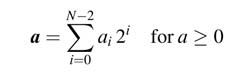
Therefore the two’s complement implementation of an N -bit positive number is equivalent to the (N – 1)-bit unsigned value of the number. In this representation, 0 is considered as a positive number. The range of positive numbers that can be represented in N bits is from 0 to (2N – 1 – 1).
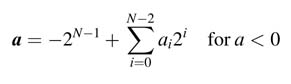
For negative numbers, the MSB aN –1 = 1 has a negative weight and all the other bits have positive weight. A closed-form expression of a two’s complement negative number is:
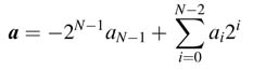
Combining (3.1) and (3.2) into (3.3) gives a unified representation to two’s complement numbers:
It is also interesting to observe an unsigned equivalent of negative two’s complement numbers. Many SW and HW simulation tools display all numbers as unsigned numbers. While displaying numbers these tools assign positive weights to all the bits of the number. The equivalent unsigned representation of negative numbers is given by:
where a is equal to the absolute value of the negative number a .
Example: –9 in a 5-bit two’s complement representation is 10111. The equivalent unsigned representation of –9 is 25 – 9 = 23.
3.3.3 Computing Two’s Complement of a Signed Number
The two’s complement of a signed number refers to the negative of the number. This can be computed by inverting all the bits and adding 1 to the least significant bit (LSB) position of the number. This is equivalent to inverting all the bits while moving from LSB to MSB and leaving the least significant 1 as it is. From the hardware perspective, adding 1 requires an adder in the HW, which is an expensive preposition. Chapter 5 covers interesting ways of avoiding the adder while computing the two’s complement of a number in HW designs.
Example: The 4-bit two’s complement representation of –2 is 4'b 1110, its 2's complement is obtained by inverting all the bits, into 4'b 0001, and adding 1 to that inverted number giving 4'b0010.
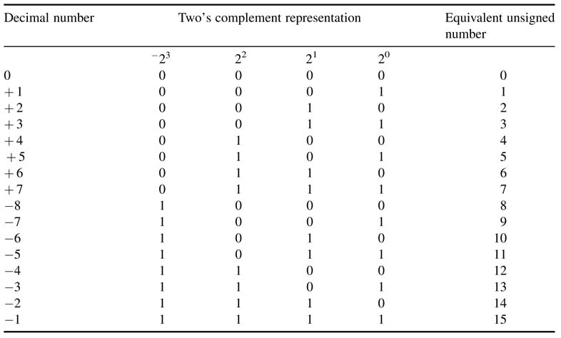
Table 3.3 lists the two’s complement representations of 4 bit numbers and their unsigned equivalent numbers. In two’s complement, the representation of a negative number does look odd because after 7 comes –8, but it facilitates the hardware implementation of many basic arithmetic operations. For this reason, this representation is used widely for executing arithmetic operations in special algorithms and general-purpose architectures.
It is apparent from (3.3) above that the MSB position plays an important role in two’s complement representation of a negative number and directly affects many arithmetic operations. While implementing algorithms using two’s complement arithmetic, a designer needs to deal with the issue of overflow. An overflow occurs if a calculation generates a number that cannot be represented using the assigned number of bits in the number. For example, 7 + 1=8, and 8 cannot be represented as a 4-bit signed number. The same is the case with –9, which may be produced as (–8) – 1.
Table 3.3 Four-bit representation of two’s complement number and its equivalent unsigned number
3.3.4 Scaling
While implementing algorithms using finite precision arithmetic it is sometimes important to avoid overflow as it adds an error that is equal to the complete dynamic range of the number. For example, the case 7 + 1 = 8 = 4'b 1000 as a 4-bit signed number is – 8. To avoid overflow, numbers are scaled down. In digital designs it is sometimes also required to sign extend an N -bit number to an M -bit number for M> N.
3.3.4.1 Sign Extension
In the case of a signed number, without affecting the value of the number, M – N bits are sign extended. Thus a number can be extended by any number of bits by copying the sign bit to extended bit locations. Although this extension does not change the value of the number, its unsigned equivalent representation will change. The new equivalent number will be:

Example: The number –2 as a 4-bit binary number is 4'b 1110. As an 8-bit number it is 8'b 11111110.
3.3.4.2 Scaling-down
When a number has redundant sign bits, it can be scaled down by dropping the redundant bits. This dropping of bits will not affect the value of the number.
Example: The number –2 as an 8-bit two’s complement signed number is 8'b 11111110. There are six redundant sign bits. The number can be easily represented as a 2-bit signed number after throwing away six significant bits. The truncated number in binary is 2'b 10.
3.4 Floating-point Format
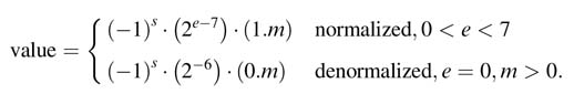
Floating-point representation works well for numbers with large dynamic range. Based on the number of bits, there are two representations in IEEE 754 standard [9]: 32-bit single-precision and 64-bit double-precision. This standard is almost exclusively used across computing platforms and hardware designs that support floating-point arithmetic. In this standard a normalized floating-point number x is stored in three parts: the sign s , the excess exponent e , and the significand or mantissa m , and the value of the number in terms of these parts is:
This indeed is a sign magnitude representation, s represents the sign of the number and m gives the normalized magnitude with a 1 at the MSB position, and this implied 1 is not stored with the number. For normalized values, m represents a fraction value greater than 1.0 and less than 2.0. This IEEE format stores the exponent e as a biased number that is a positive number from which a constant bias b is subtracted to get the actual positive or negative exponent.
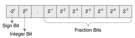
Figure 3.2 shows this representation for a single-precision floating point number. Such a number is represented in 32 bits, where 1 bit is kept for the sign s, 8 bits for the exponent e and 23 bits for the mantissa m. For a 64-bit double-precision floating-point number, 1 bit is kept for the sign,11 bits for the exponent and 52 bits for the mantissa. The values of bias b are 127 and 1023, respectively, for single-and double-precision floating-point formats.
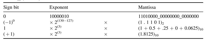
Example: Find the value of the following 32-bit binary string representing a single-precision IEEE floating-point format: 0_10000010_11010000_00000000_0000000. The value is calculated by parsing the number into different fields, namely sign bit, exponent and mantissa, and then computing the value of each field to get the final value, as shown in Table 3.4.
Example: This example represents –12.25 in single-precision IEEE floating-point format. The number –12.25 in sign magnitude binary is –00001100.01. Now moving the decimal point to bring it into the right format: –1100.01 ×20 =–1.10001 × 23. Thus the normalized number is – 1.10001 × 23.
Sign bit (s) = 1
Mantissa field(m) = 10001000_00000000_0000000
Exponent field(e) = 3 + 127 = 130 = 82 h = 1000 0010
So the complete 32-bit floating-point number in binary representation is:
1_10000010_1000100_000000000_0000000
Figure 3.2 IEEE format for single-precision 32-bit floating point number
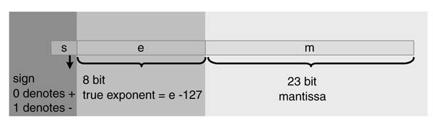
Table 3.4 Value calculated by parsing and then computing the value of each field to get the final value, 14.5 (see text)
A floating-point number can also overflow if its exponent is greater or smaller than the maximum or minimum value the e-field can represent. For IEEE single-precision floating point format, the minimum to maximum exponent ranges from 2–126 to 2127. On the same account, allocating 11 bits in the e-field as opposed to 8 bits for single-precision numbers, minimum and maximum values of a double-precision floating-point number ranges from 2–1022 to 21023
Although the fields in the format can represent almost all numbers, there are still some special numbers that require unique handling. These are:
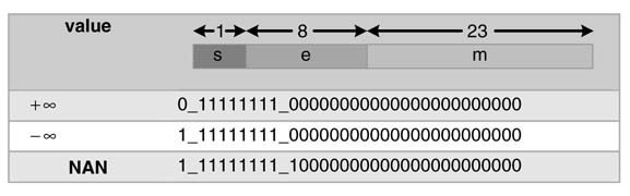
A ± ∞ may be produced if any floating-point number is divided by zero, so 1.0/0.0= + ∞. Similarly, –1.0/0.0 = – ∞. Not A Number (NAN) is produced for an invalid operations like 0/0 or ∞ – ∞.
3.4.1 Normalized and Denormalized Values
The floating-point representation covers a wide dynamic range of numbers. There is an extent where the number of bits in the mantissa is enough to represent the exact value of the floating-point number and zero placed in the exponent. This range of values is termed denormalized. Beyond this range, the representation keeps normalizing the number by assigning an appropriate value in the exponent field. A stage will be reached where the number of bits in the exponent is not enough to represent the normalized number and results in + ∞ or – ∞. In instances where a wrong calculation is conducted, the number is represented as NAN. This dynamic range of floating-point representation is shown in Figure 3.3.
In the IEEE format of floating-point representation, with an implied 1 in the mantissa and a nonzero value in the exponent, where all bits are neither 0 nor 1, are called normalized values. Denormalized values are values where all exponent bits are zeros and the mantissa is non-zero.
Figure 3.3 Dynamic range of a floating-point number
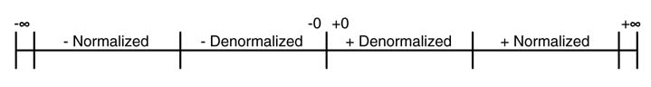
These values represent numbers in the range of zero and smallest normalized number on the number line:
The example below illustrates normalized and denormalized numbers.
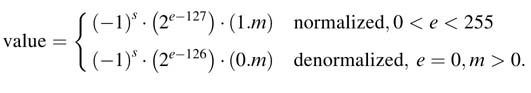
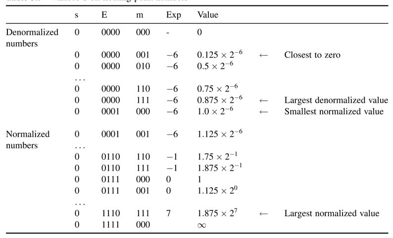
Example : Assume a floating-point number is represented as an 8-bit number. There is one sign bit and 4 and 3 bits, respectively, are allocated to store exponent and mantissa. By traversing through the entire range of the number, limits for denormalized and normalized values can be easily marked. The value where the e-field is all zeros and the m-field is non-zero represents denormalized values. This value does not assume an implied 1in the mantissa. For a normalized value an implied 1 is assumed and a bias of + 7 is added in the true exponent to get the e-field .Therefore for a normalized value this bias is subtracted from the e-field to get the actual exponent. These numbers can be represented as:
The ranges of positive denormalized and normalized numbers for 8-bit floating-point format are given in Table 3.5.
Floating-point representation works well where variables and results of computation may vary over a large dynamic range. In signal processing, this usually is not the case. In the initial phase of algorithm development, though, before the ranges are conceived, floating-point format gives comfort to the developer as one can concentrate more on the algorithmic correctness and less on implementation details. If there are no strict requirements on numerical accuracy of the computation, performing floating-point arithmetic in HW is an expensive preposition in terms of power, area and performance, so is normally avoided. The large gate densities of current generation FPGAs and ASICs allow designers to map floating-point algorithms in HW if required. This is especially true for more complex signal processing applications where keeping the numerical accuracy intact is considered critical [10].
Table 3.5 Various 8-bit floating-point numbers
Floating-point arithmetic requires three operations: exponent adjustment, mathematical operation, and normalization. Although no dedicated floating-point units are provided on FPGAs, embedded fast fixed-point adder/subtractors, multipliers and multiplexers are used in effective floating-point arithmetic units [11].
3.4.2 Floating-point Arithmetic Addition
The following steps are used to perform floating-point addition of two numbers:
S0 Append the implied bit of the mantissa. This bit is 1 or 0 for normalized and denormalized numbers, respectively.
S1 Shift the mantissas from S0 with smaller exponent es to the right by el - es, where el is the larger of the two exponents. This shift may be accomplished by providing a few guard bits to the right for better precision.
S2 If any of the operands is negative, take two’s complement of the mantissa from S1 and then add the two mantissas. If the result is negative, again takes two’s complement of the result.
S3 Normalize the sum back to IEEE format by adjusting the mantissa and appropriately changing the value of the exponent el . Also check for underflow and overflow of the result.
S4 Round or truncate the resultant mantissa to the number of bits prescribed in the standard.
Example: Add the two floating-point numbers below in 10-bit precision, where 4 bits are kept for the exponent, 5 bits for the mantissa and 1 bit for the sig. Assume the bias value is 7:
0_1010_00101
0_1001_00101
Taking the bias + 7 off from the exponents and appending the implied 1, the numbers are:
1.00101b ×23 and 1.00101b× 22
S0 As both the numbers are positive, there is no need to take two’s complements. Add one extra bit as guard bit to the right, and align the two exponents by shifting the mantissa of the number with the smaller exponent accordingly:
1.00101b × 23→1.001010b × 23
1.00101b × 22→ 0.100101b × 23
S 1 Add the mantissas:
1.001010b + 0.100101b = 1.101111b
S 2 Drop the guard bit:
1.10111b × 23
S 3 The final answer is 1.10111b × 23, which in 10-bit format of the operands is 0_1010_10111.
3.4.3 Floating-point Multiplication
The following steps are used to perform floating-point multiplication of two numbers.
S0 Add the two exponents e1 and e2. As inherent bias in the two exponents is added twice, subtract the bias once from the sum to get the resultant exponent e in correct format.
S1 Place the implied 1 if the operands are saved as normalized numbers. Multiply the mantissas as unsigned numbers to get the product, and XOR the two sign bits to get the sign of the product.
S2 Normalize the product if required. This puts the result back to IEEE format. Check whether the result underflows or overflows.
S3 Round or truncate the mantissa to the width prescribed by the standard.
Example: Multiply the two numbers below stored as 10-bit floating-point numbers, where 4 bits and 5 bits, respectively, are allocated for the exponent and mantissa, 1 bit is kept for the sign and 7 is used as bias:
3.5 → 0_1000_11000
5.0 → 0_1001_01000
S0 Add the two exponents and subtract the bias 7 (=0111) from the sum:
1000+ 1001—0111 = 1010
S1 Append the implied 1 and multiply the mantissa using unsigned × unsigned multiplication:
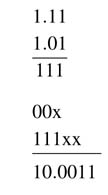
S2 Normalize the result:
(10:0011)b× 23→(1:00011)b × 24
(1:00011)b× 24→(17:5)10
S3 Put the result back into the format of the operands. This may require dropping of bits but in this case no truncation is required and the result is (1.00011)b × 2 stored as 0_1011_00011.
3.5 Qn.m Format for Fixed-point Arithmetic
3.5.1 Introducing Qn.m
Most signal processing and communication systems are first implemented in double-precision floating-point arithmetic using tools like MATLAB®. While implementing these algorithms the main focus of the developer is to correctly assimilate the functionality of the algorithm. This MATLAB® code is then converted into floating-point C/C ++ code. C++ code usually runs much faster than MATLAB® routines. This code conversion also gives more understanding of the algorithm as the designer might have used several functions from MATLAB® toolboxes. Their understanding is critical for porting these algorithms in SW or HW for embedded devices. After getting the desired performance from the floating-point algorithm, this implementation is converted to fixed-point format. For this the floating-point variables and constants in the simulation are converted to Qn.m fixed-point format. This is a fixed positional number system for representing floating-point numbers
Figure 3.4 Fields of the bits and their equivalent weights for the text example
The Qn.m format of an N -bit number sets n bits to the left and m bits to the right of the binary point. In cases of signed numbers, the MSB is used for the sign and has negative weight. A two’s complement fixed-point number in Qn.m format is equivalent to b = bn – 1 ,bn –2…b1 b0 b-1 b-2…b –m , with equivalent floating point value:

Example: Compute the floating-point equivalent of 01_1101_0000 in signed Q2.8 format. The fields of the bits and their equivalent weights are shown in Figure 3.4.
Assigning values to bit locations gives the equivalent floating-point value of the Q-format fixed-point number:
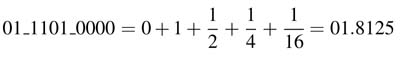
This example keeps 2 bits to store the integer part and the remaining 8 bits are for the decimal part. In these 10 bits the number covers –2 to + 1.9961.
3.5.2 Floating-point to Fixed-point Conversion of Numbers
Conversion requires serious deliberation as it results in a tradeoff between performance and cost. To reduce cost, shorter word lengths are used for all variables in the code, but this adversely affects the numerical performance of the algorithm and adds quantization noise.
A floating-point number is simply converted to Qn.m fixed-point format by brining m fractional bits of the number to the integer part and then dropping the rest of the bits with or without rounding. This conversion translates a floating-point number to an integer number with an implied decimal. This implied decimal needs to be remembered by the designer for referral in further processing of the number in different calculations:
Num_fixed = round(num_float × 2m)
or num_fixed = fix (num_float × 2m)
The result is saturated if the integer part of the floating-point number is greater than n. This is simply checked if the converted fixed-point number is greater than the maximum positive or less than the minimum negative N-bit two’s complement number. The maximum and minimum values of an N -bit two’s complement number are 2N-1 – 1 and –2N-1 , respectively.
num_fixed = round(num_float x2m )
if (num_fixed > 2N-1 -1)
num_fixed = 2 N-1 -1
elseif (num_fixed < -2 N-1)
num_fixed = -2N-1
Example: Most commercially available off-the-shelf DSPs have 16-bit processors. Two examples of these processors are the Texas Instruments TMS320C5514 and the Analog Devices ADSP-2192. To implement signal processing and communication algorithms on these DSPs, Q1.15 format (commonly known as Q15 format) is used. The following pseudo-code describes the conversion logic to translate a floating-point number num_float to fixed-point number num_fixed_Q15 in Q1.15 format:
Num_fixed_long = (long)(num_float×215)
if (num fixed long > 0x7fff)
num fixed long = 0x7fff
elseif (num fixed long < 0xffff8000)
num_fixed_long =0xffff8000
num_fixed_Q15 = (short)(num_fixed_long & 0xffff))
Using this logic, the following lists a few floating-point numbers (num_float) and their representation in Q1.15 fixed-point format (num_fixed_Q15) :
0.5→ 0x4000
–0.5→ 0xC000
0.9997 → 0x7FF6
0.213 → 0x1B44
–1.0 → 0x8000
3.5.3 Addition in Q Format
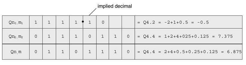
Addition of two fixed-point numbers a and b of Q n 1.m1 and Qn2.m2 formats, respectively, results in a Qn.m format number, where n is the larger of n 1 and n2 and m is the larger of m 1and m2. Although the decimal is implied and does not exist in HW, the designer needs to align the location of the implied decimal of both numbers and then appropriately sign extend the number that has the least number of integer bits. As the fractional bits are stored in least significant bits, no extension of the fractional part is required. The example below illustrates Q-format addition.
Example: Add two signed numbers a and b in Q2.2 and Q4.4 formats. In Q2.2 format a is 1110, and in Q4.4 format b is 0111_0110. As n 1 is less than n2, the sign bit of a is extended to change its format from Q2.2 to Q4.2 (Figure 3.5). The extended sign bits are shown with bold letters. The numbers are also placed in such a way that aligns their implied decimal point. The addition results in a Q4.4 format number.
3.5.4 Multiplication in Q Format
If two numbers a and b in, respectively, Qn 1.m1 and Qn2.m2 formats are multiplied, the multiplication results in a product in Q(n 1 +n2).(m1 + m2) format. If both numbers are signed two’s complement numbers, we get a redundant sign bit at the MSB position. Left shifting the product by 1 removes the redundant sign bit, and the format of the product is changed to Q(n 1 +n2 — 1).(m 1 + m2 + 1). Below are listed multiplications for all possible operand types.
Figure 3.5 Example of addition in Q format
3.5.4.1 Unsigned by Unsigned
Multiplication of two unsigned numbers in Q2.2 and Q2.2 formats results in a Q4.4 format number, as shown in Figure 3.6. As both numbers are unsigned, no sign extension of partial products is required. The partial products are simply added. Each partial product is sequentially generated and successively shifted by one place to the left.
3.5.4.2 Signed by Unsigned
Multiplication of a signed multiplicand in Q2.2 with an unsigned multiplier in Q2.2 format results in a Q4.4 format signed number, as shown in Figure 3.7. As the multiplicand is a signed number, this requires sign extension of each partial product before addition. In this example the partial products are first sign-extended and then added. The sign extension bits are shown in bold.
Figure 3.6 Multiplication, unsigned by unsigned
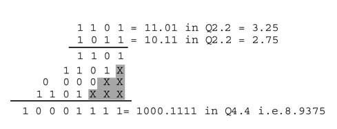
Figure 3.7 Multiplication, signed by unsigned
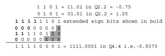
Figure 3.8 Multiplication, unsigned by signed
3.5.4.3 Unsigned by Signed
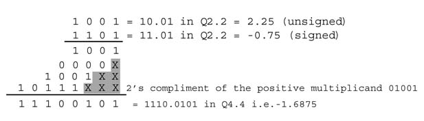
Multiplication of an unsigned multiplicand in Q2.2 with a signed multiplier in Q2.2 format results in a Q4.4 format signed number, as shown in Figure 3.8. In this case the multiplier is signed and the multiplicand is unsigned. As all the partial products except the final one are unsigned, no sign extension is required except for the last one. For the last partial product the two’s complement of the multiplicand is computed as it is produced by multiplication with the MSB of the multiplier, which has negative weight. The multiplicand is taken as a positive 5-bit number, 01001, and its two’s complement is 10111.
3.5.4.4 Signed by Signed
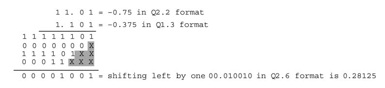
Multiplication of a signed number in Q1.2 with a signed number in Q1.2 format results in a Q1.5 format signed number, as shown in Figure 3.9. Sign extension of partial products is again necessary. This multiplication also produces a redundant sign bit, which can be removed by left shifting the result. Multiplying a Qn 1.m1 format number with a Qn2.m2 number results in a Q(n 1 +n2).(m1 + m2) number, which after dropping the redundant sign bit becomes a Q(n 1 +n2–1).(m1 + m2 + 1) number.
The multiplication in the example results in a redundant sign bit shown in bold. The bit is dropped by a left shift and the final product is 111000 in Q1.5 format and is equivalent to —0.25.
When the multiplier is a negative number, while calculating the last partial product (i.e. multiplying the multiplicand with the sign bit with negative weight), the two’s complement of the multiplicand is taken for the last partial product, as shown in Figure 3.10.
Figure 3.9 Multiplication, signed by signed
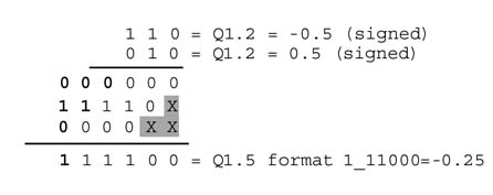
Figure 3.10 Multiplication, signed by signed
3.5.5 Bit Growth in Fixed-point Arithmetic
Bit growth is one of the most critical issues in implementing algorithms using fixed-point arithmetic. Multiplication of an N-bit number with an M-bit number results in an (N + M )-bit number, a problem that grows in recursive computations. For example, implementing the recursive equation:
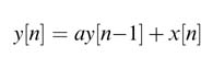
requires multiplication of a constant a with a previous value of the output y[n – 1]. If the first output is an N -bit number in Qn 1.m1 format and the constant a is an M -bit number in Qn2.m2 format, in the first iteration the product ay[n – 1] is an (N + M )-bit number in Q(n 1 + n2 – 1).(m 1 +m2 + 1) format. In the second iteration the previous value of the output is now an N + M bits, and once multiplied by a it becomes N + 2M bits. The size will keep growing in each iteration. It is therefore important to curtail the size of the output. This requires truncating the output after every mathematical operation. Truncation is achieved by first rounding and then dropping a defined number of least significant bits or without rounding dropping these bits.
The bit growth problem is also observed while adding two different Q-format numbers. In this case the output format of the number will be:
Assigning an appropriate format to the output is very critical and one can use Schwarz’s inequality of (3.9) to find an upper bound on the output values of a linear time-invariant (LTI) system:
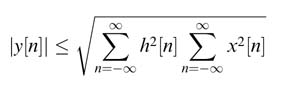
Here h [n ] and x [n ] are impulse response and input to an LTI system, respectively. This helps the designer to appropriately assign bits to the integer part of the format defined to store output values. Assigning bits to the fraction part requires deliberation as it depends on the tolerance of the system to quantization noise.
Example: Adding an 8-bit Q7.1 format number in an 8-bit Q1.7 format number will yield a 14-bit Q7.7 format number.
Figure 3.11 Rounding followed by truncation
3.5.5.1 Simple Truncation
In multiplication of two Q-format numbers, the number of bits in the product increases. The precision is sacrificed by dropping some low-precision bits of the product: Qn 1.m 1 is truncated to Qn 1.m 2, where m 2 <m 1.
Example:
0111_0111 in Q4.4 is 7.4375
Truncated to Q4.2 gives 0111_01 = 7.25
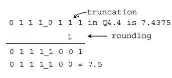
3.5.5.2 Rounding Followed by Truncation
Direct truncation of numbers biases the results, so in many applications it is preferred to round before trimming the number to the desired size. For this, 1 is added to the bit that is at the right of the position of the point of truncation. The resultant number is then truncated to the desired number of bits. This is shown in the example in Figure 3.11. First rounding and then truncation gives a better approximation; in the example, simple truncation to Q4.2 results in a number with value 7.25, whereas rounding before truncation gives 7.5 – which is closer to the actual value 7.4375.
3.5.6 Overflow and Saturation
Overflow is a serious consequence of fixed-point arithmetic. Overflow occurs if two positive or negative numbers are added and the sum requires more than the available number of bits. For example, in a 3-bit two’s complement representation, if 1 is added to 3 (=3'b 011), the sum is 4 (= 4'b 0100). The number 4 thus requires four bits and cannot be represented as a 3-bit two’s complement signed number as 3'b 100 (=–4). This causes an error equal to the full dynamic range of the number and so adversely affects subsequent computation that uses this number.
Figure 3.12 shows the case of an overflow for a 3-bit number, adding an error equal to the dynamic range of the number. It is therefore imperative to check the overflow condition after performing arithmetic operations that can cause a possible overflow. If an overflow results, the designer should set an overflow flag. In many circumstances, it is better to curtail the result to the maximum positive or minimum negative value that the defined word length can represent. In the above example the value should be limited to 3'b 011.
Thus, the following computation is in 3-bit precision with an overflow flag set to indicate this abnormal result:
3 + 1 = 3 and overflow flag = 1
Similarly, performing subtraction with an overflow flag set to ! is:
–4– 1 = –4 overflow flag = 1
Figure 3.12 Overflow and saturation. (a) Overflow introduces an error equal to the dynamic range of the number. (b) Saturation clamps the value to a maximum positive or minimum negative level
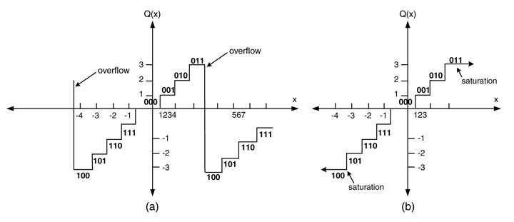
Figure 3.12 shows the overflow and saturation mode for 3-bit two’s complement numbers, respectively. The saturation mode clamps the value of the number to the maximum positive or minimum negative.
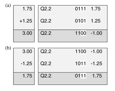
The designer may do nothing and let the overflow happen, as shown in Figure 3.13(a). For the same calculation, the designer can clamp the answer to a maximum positive value in case of an overflow, as shown in Figure 3.13(b).
3.5.7 Two’s Complement Intermediate Overflow Property
In an iterative calculation using two’s complement arithmetic, if it is guaranteed that the final result will be within the precision bound of the assigned fixed-point format, then any amount of intermediate overflows will not affect the final answer.
This property is illustrated in Figure 3.14(a) with operands representing 4-bit precision. The first column shows the correct calculation but, owing to 4-bit precision, the result overflows and the calculation yields an incorrect answer as shown in the third column. If the further calculation uses this incorrect answer and adds a value that guarantees to bring the final answer within the legal limits of the format, then this calculation will yield the correct answer even though one of the operands in the calculation is incorrect. The calculation in Figure 3.14(b) shows that even using the incorrect value from the earlier calculation the further addition will yield the right value.
Figure 3.13 Handling overflow: (a) doing nothing; (b) clamping
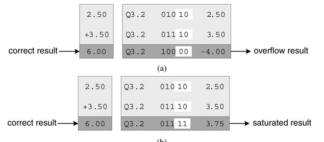
Figure 3.14 Two’s complement intermediate overflow property: (a) incorrect intermediate result; (b) correct final result
This property of two’s complement arithmetic is very useful in designing architectures. The algorithms in many design instances can guarantee the final output to fit in a defined format with possible intermediate overflows.
3.5.7.1 CIC Filter Example
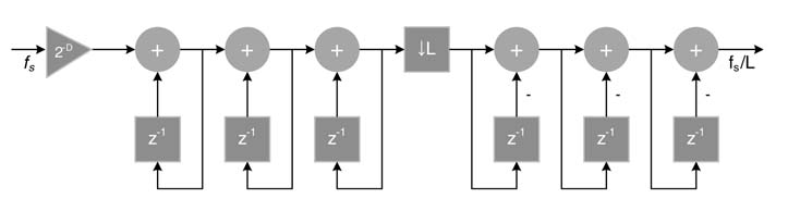
The above property can be used effectively if the bounds on output can be determined. Such is the case with a CIC (cascaded integrator-comb) filter which is an integral part of all digital down-converters. A CIC filter has M stages of integrator executing at sampling rate f s, followed by a decimator by a factor of L , followed by a cascade of M stages of Comb filter running at decimated sampling rate f s/L . The transfer function of such a CIC filter is:
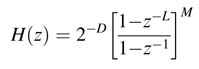
It is proven for a CIC filter that, for signed input of Qn.m format, the output also fits in Qn.m format provided each input sample is scaled by a factor of D , where:
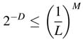
M is the order ofthe filter. ACIC filterisshown in Figure 3.15.In this design, provided the input is scaled by a factor of D , then intermediate values may overflow any amount of times and the output remains within the bounds of the Qn.m format.
3.5.7.2 FIR Filter Example
If all the coefficients of an FIR (finite impulse response)filter are scaled tofitinQ1.15 format, and the filter design package ensures that the sum of the coefficients is 1, then fixed-point implementation of the filter does not overflow and uses the complete dynamic range of the defined format.
Figure 3.15 An M th-order CIC filter for decimating a signal by a factor of L (here, M — 3). The input is scaled by a factor of D to avoid overflow of the output. Intermediate values may still overflow a number of times but the output is always correct
The output can be represented in Q1.15 format. MATLAB® filter design utilities guarantee that the sum of all the coefficients of an FIR filter is 1; that is:
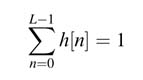
where L is the length of the filter. This can be readily checked in MATLAB® for any amount of coefficients and cutoff frequency, as is done below for a 21-coefficient FIR filter with cutoff frequency π /L:
>> sum(fir1(20,.1))
ans =
1.0000
3.5.8 Corner Cases
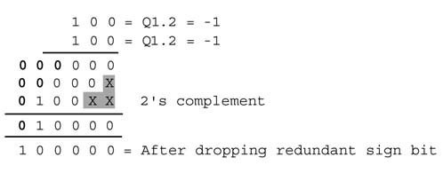
Two’s complement arithmetic has one serious shortcoming, in that in N -bit representation of numbers it does not have an equivalent opposite of –2N - 1 . For example, for a 4-bit signed number there is no equivalent opposite of –16, the maximum 4-bit positive number being + 15. This is normally referred to as a corner case, and the digital designer needs to be concerned with the occurrence of this in computations. Multiplying two signed numbers and dropping the redundant sign bit may also result in this corner case.
For example, consider multiplying –1 by –1 in Q1.2 format, as shown in Figure 3.16. After throwing away the redundant sign bit the answer is 100000 (=–1) in Q1.5 format, which is incorrect. The designer needs to add an exclusive logic to check this corner case, and if it happens saturate the result with a maximum positive number in the resultant format.
Figure 3.16 Multiplying –1 by –1 in Q1.2 format
The following C code shows fixed-point multiplication of two 16-bit numbers, where the result is saturated if multiplication results in this corner case.
Word32 L_mult(Word16 var1,Word16 var2)
{
 Word32 L_var_out;
 L_var_out= (Word32)var1 * (Word32)var2;
 // Sign*sing multiplication
/*
Check corner case. If before throwing away redundant sign bit the answer is 0x40000000, it is the corner case, so set the overflow flag and clamp the value to maximum 32-bit positive number in fixed-point format.
*/
 if (L_var_out != (Word32)0x40000000L) // 8000H*8000H=40000000Hex
 {
 L_var_out *= 2; //Shift the redundant sign bit out
 }
 else
 {
 Overflow = 1;
 L_var_out = 0x7fffffff;
 //If overflow then clamp the value to MAX_32
 }
 return(L_var_out);
}
3.5.9 Code Conversion and Checking the Corner Case
The C code below implements the dot-product of two arrays h_float and x_float :
float dp_float (float x[], float h[], int size)
{
 float acc;
 int i;
 acc = 0;
 for(i = 0; i < size; i++)
 {
 acc+=x[i] *h[i];
 }
 return acc;
}
Let the constants in the two arrays be:
float h_float[SIZE] = {0.258, -0.309, -0.704, 0.12};
float x_float[SIZE]= {-0.19813, -0.76291,0.57407,0.131769);
As all the values in the two arrays h_float and x_float are bounded within + 1 and –1, an appropriate format for both the arrays is Q1.15. The arrays are converted into this format by multiplying by 215 and rounding the result to change these numbers to integers:
Short h16[SIZE] = {8454, -10125, -23069, 3932};
Short x16[SIZE] = {-6492, -24999, 18811, 4318};
The following C code implements the same functionality in fixed-point format assuming short and int are 16-bit and 32-bit wide, respectively:
int dp_32(short x16[ ], shorth16[ ], int size)
{
 int prod32;
 int acc32;
 int tmp32;
 int i;
 acc32 = 0;
 for ( i = 0 ; i < size ; i++ )
 {
 prod32 = x16 [i] * h16 [i] ; //Q2.30 = Q1.15 * Q1.15
 if (prod32 == 0x40000000) // saturation check
 prod32 = MAX_32;
 else
 prod32 <<= 1; // Q1.31 = Q2.31 <<1;
 tmp32 = acc32 + prod32; // accumulator
 // +ve saturation logic check
 if(((acc32>0) 0))
 acc32 = MAX_32;
 // Negative saturation logic check
 else if(((acc32<0) && (prod32< 0) ) && (tmp32>0))
 acc32 =MIN_32;
 // The case of no overflow
 else
 acc32 = tmp32;
 }
}
As is apparent from the C code, fixed-point implementation results in several checks and format changes and thus is very slow. In almost all fixed-point DSPs the provision of shifting out redundant sign bits in cases of sign multiplication and checking of overflow and saturating the results are provided in hardware.
3.5.10 Rounding the Product in Fixed-point Multiplication
The following C code demonstrates complex fixed-point multiplication for Q1.15-format numbers. The result is rounded and truncated to Q1.15 format:
typedef struct COMPLEX_F
{
 short real;
 short imag;
}
COMPLEX_F;
COMPLEX_F ComplexMultFixed (COMPLEX_F a, COMPLEX_F b)
{
COMPLEX_F out;
Int L1, L2, tmp1, tmp2;
L1 = a.real * b.real;
L2 = a.imag * b.imag;
// Rounding and truncation
out.real=(short) (((L1 - L2)+0x00004000)>>15);
L1 = a.real * b.imag;
L2 = a.imag * b.real;
// Rounding and truncation
out.imag=(short) (((L1 + L2)+0x00004000)>>15
return (out);
}
3.5.10.1 Unified Multiplier
From the hardware design perspective, placing four separate multipliers to cover general multiplication is an expensive proposition. A unified multiplier can handle all the four types of multiplication. For N1 ×N2 multiplication, this is achieved by appending one extra bit to the left of the MSB of both of the operands. When an operand is unsigned, the extended bit is zero, otherwise the extended bit is the sign bit of the operand. This selection is made using a multiplexer (MUX). The case for a 16 × 16 unified multiplier is shown in Figure 3.17.
After extending the bits, (N 1 + 1) ×(N2 + 1) signed by signed multiplication is performed and only N 1 ×N2 bits of the product are kept for the result. Below are shown four options and their respective modified operands for multiplying two 16-bit numbers, a and b:
Figure 3.17 One-bit extension to cater for all four types of multiplications using a single signed by signed multiplier
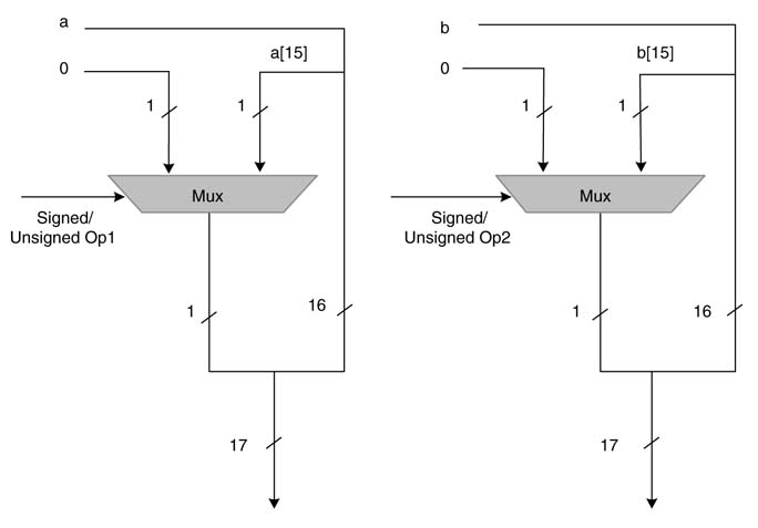
unsigned by unsigned: {1′b 0, a }, {1′b 0, b }
unsigned by signed: {1′b 0, a }, {b [15], b }
signed by unsigned: {a [15], a }, {1′b 0, b }
signed by signed: {a [15], a }, {b [15], b }.
Further to this, there are two main options for multiplications. One option multiplies integer numbers and the second multiplies Q-format numbers. The Q-format multiplication is also called fractional multiplication . In fractional signed by signed multiplication, the redundant sign bit is dropped, whereas for integer sign by sign multiplication this bit is kept in the product.
A unified multiplier that takes care of all types of signed and unsigned operands and both integer and fractional multiplication is given in Figure 3.18. The multiplier appropriately extends the bits of the operands to handle signed and unsigned operands, and in the case of fractional sign by sign multiplication it also drops the redundant sign bit.
Figure 3.18 Unified multiplier for signed by signed, signed by unsigned, unsigned by unsigned and unsigned by signed multiplication for both fraction and integer modes, it also cater for the corner case
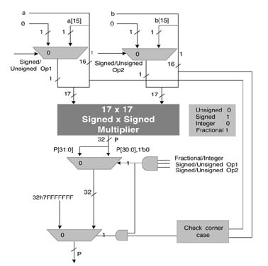
Figure 3.19 Demonstration of the difference between integer and fractional multiplication
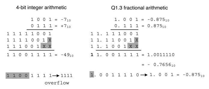
In many designs the result of multiplication of two N -bit numbers is rounded to an N -bit number. This truncation of the result requires separate treatment for integer and fractional multipliers.
- For integer multiplication, the least significant N bits are selected for the final product provided the most significant N bits are redundant sign bits. If they are not, then the result is saturated to the appropriate maximum or minimum level.
- For fractional multiplication, after dropping the redundant sign bit and adding a 1 to the seventeenth bit location for rounding, the most significant N bits are selected as the final product.
The difference between integer and fractional multiplication is illustrated in Figure 3.19. The truncated product in integer multiplication overflows and is 11112 = – 110. The product for factional multiplication, after dropping the sign bit out by shifting the product by 1 to the left and then dropping the four LSBs, is –0.875.
3.5.11 MATLAB® Support for Fixed-point Arithmetic
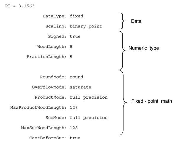
MATLAB® provides the fi tool that is a fixed-point numeric object with a complete list of attributes that greatly help in seamless conversion of a floating-point algorithm to fixed-point format. For example, using fi (), π is converted to a signed fixed-point Q3.5 format number:
>>PI=fi(pi, 1, 3+5, 5);% Specifying N bits and the fraction part
>> bin(PI)
01100101
>> double(PI)
 3.1563
All the available attributes that a programmer can set for each fixed-point object are given in Figure 3.20.
Figure 3.20 support for fixed-point arithmetic
3.5.12 SystemC Support for Fixed-point Arithmetic
As with MATLAB®, once a simulation is working in SystemC using double-precision floating-point numbers, by merely substituting or redefining the same variable with fixed-point attributes the same code can be used for fixed-point implementation. This simple conversion greatly helps the developer to explore a set of word lengths and rounding or truncation options for different variables by changing the attributes.
Here we look at an example showing the power of SystemC for floating-point and fixed-point simulation. This program reads a file with floating-point numbers. It defines a fixed-point variable fx_value in Q6.10 with simple truncation and saturation attributes. The program reads a floating-point value in a fp_value variable originally defined as of type double, and a simple assignment of this variable to fx_value changes the floating-point value to Q6.10 format by rounding the number to 16 bits; and when the integer part is greater than what the format can support the value is saturated. SystemC supports several options for rounding and saturation.
intsc_main (intargc, char *argv[])
{
sc_fixed <16,6, SC_TRN, SC_SAT>fx_value;
double fp_value;
int i, size;
 ofstream fout("fx_file.txt");
 ifstream fin("fp_file.txt");
 if (fin.is_open())
 fin >> size;
 else
 cout << "Error opening input file!
";
 cout << "size = " << size << endl;
for (i=0; i<size; i++)
{
 if (!fin.eof())
 {
 fin >> fp_value;
 fx_value = fp_value;
 cout << "double = " << fp_value"	 fixpt = " << fx_value<< endl;
 fout << fx_value<< endl;
 }
 }
}
Table 3.6 shows the output of the program.
Table 3.6 Output of the program in the text
| double = 0.324612 | fixpt = 0.3242 |
| double = 0.243331 | fixpt = 0.2432 |
| double = 0.0892605 | fixpt = 0.0889 |
| double = 0.8 | fixpt = 0.7998 |
| double =-0.9 | fixpt =–0.9004 |
3.6 Floating-point to Fixed-point Conversion
Declaring all variables as single- or double-precision floating-point numbers is the most convenient way of implementing any DSP algorithm, but from a digital design perspective the implementation takes much more area and dissipates a lot more power than its equivalent fixed-point implementation. Although floating-point to fixed-point conversion is a difficult aspect of algorithm mapping on architecture, to preserve area and power this option is widely chosen by designers.
For fixed-point implementation on a programmable digital signal processor, the code is converted to a mix of standard data types consisting of 8-bit char, 16-bit short and 32-bit long. Hence, defining the word lengths of different variables and intermediate values of all computations in the results, which are not assigned to defined variables ,is very simple. This is because in most cases the option is only to define them as char, short or long. In contrast, if designer’s intention is to map the algorithm on an application-specific processor then a run of optimization on these data types can further improve the implementation. This optimization step tailors all variables to any arbitrary length variables that just meet the specification and yields a design that is best from area, power and speed.
It is important to understand that a search for an optimal world length for all variables is an NP-hard problem. An exhaustive exploration of world lengths for all variables may take hours for a moderately complex design. Here, user experience with an insight into the design along with industrial practices can be very handy. The system-level design tools are slowly incorporating optimization to seamlessly evaluate a near-optimal solution for word lengths [12].
Conversion of a floating-point algorithm to fixed-point format requires the following steps [6].
S0 Serialize the floating-point code to separate each floating-point computation into an independent statement assigned to a distinct variable vari .
S1 Insert range directives after each serial floating-point computation in the serialized code of S0 to measure the range of values each distinct variable takes in a set of simulations.
S2 Design a top layer that in a loop runs the design for all possible sets of inputs. Each iteration executes the serialized code with range directives for one possible set of inputs. Make these directives keep a track of maximum max_var i and minimum min_var i values of each variable var i. After running the code for all iterations, the range directives return the range that each variable var i takes in the implementation.
S3 To convert each floating-point variable vari to fixed-point variable, fx_vari in its equivalent Qn i.m i fixed-point format, extract the integer length n i using the following mathematical relation:
S4 Setting the fractional part mi of each fixed-point variable fx_vari requires detailed technical deliberation and optimization. The integer part is critical as it must be correctly set to avoid any overflow in fixed-point computation. The fractional part, on the other hand, determines the computational accuracy of the algorithm as any truncation and rounding of the input data and intermediate results of computation appear as quantization noise. This noise, generated as a consequence of throwing away of valid part of the result after each computation, propagates in subsequent computations in the implementation. Although a smaller fractional part results in smaller area, less power dissipation and improved clock speeds, it adds quantization noise in the results.
Finding an optimal word length for each variable is a complex problem. An analytical study of the algorithm can helpindetermininganoptimal fractional part for each variabletogive acceptable ratio of signal to quantization noise (SQNR) [7]. In many design instances an analytical study of the algorithm may be too complex and involved.
An alternative to analytical study is an exhaustive search of the design space considering a pre-specified minimum to maximum fraction length of each variable. This search, even in simple design problems, may require millionsofiterationsof the algorithm and thus isnot feasibleor desirable. An intelligent trial and error method can easily replace analytical evaluation or an infeasible exhaustive search of optimal word length. Exploiting the designer’s experience, known design practices and published literature can help in coming up with just the right tailoring of the fractional part. Several researchers have also used optimization techniques like ‘mixed integer programming’ [8], ‘genetic algorithms’ [9], and ‘simulating annealing’ [10]. These techniques are slowly finding their way into automatic floating-point to fixed-point conversion utilities. The techniques are involved and require intensive study, so interested readers are advised to read relevant publications [7–12]. Here we suggest only that designer should intelligently try different word lengths and observe the trend of the SQNR, and then settle for word lengths that just give the desirable performance.
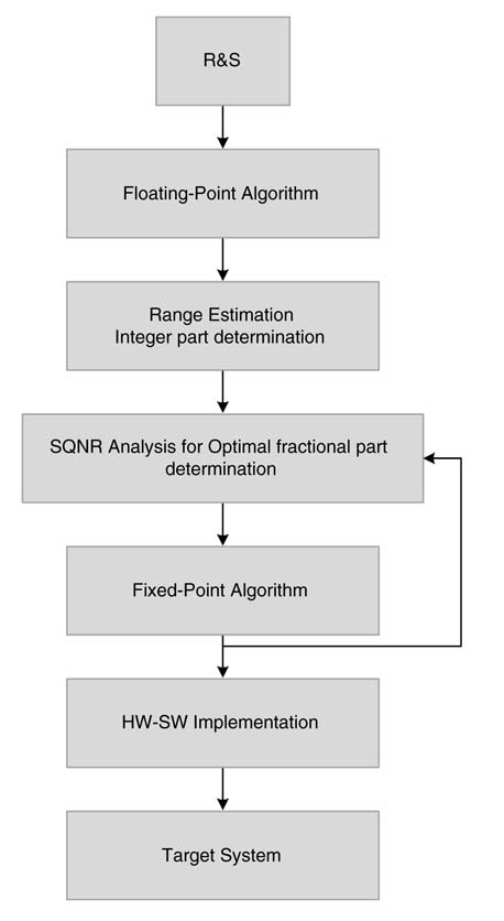
Figure 3.21 lists a sequence of steps while designing a system starting from R&S, development of an algorithm in floating point, determination of the integer part by range estimation, and then iteratively analyzing SQNR on fixed-point code to find the fractional part of Qn .m format for all numbers, and finally mapping the fixed-point algorithm on HW and SW components.
3.7 Block Floating-point Format
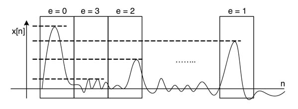
Block floating-point format improves the dynamic range of numbers for cases where a block of data goes though different stages of computation. In this format, a block of data is represented with a common exponent. All the values in the block are in fixed-point format. This format, before truncating the intermediate results, intelligently observes the number of redundant sign bits of all the values in the block, to track the value with the minimum number of redundant sign bits in the block. This can be easily extracted by computing thevalue with maximum magnitude in the block. The number of redundant sign bits in the value is the block exponent for the current block under consideration. All the values in the block are shifted left by the block exponent. This shifting replaces redundant sign bits with meaningful bits, so improving effective utilization of more bits of the representation. Figure 3.22 shows a stream of input divided into blockswith block exponent value.
Figure 3.21 Steps in system design starting from gathering R&S, implementing algorithms in floating-point format and the algorithm conversion in fixed-point while observing SQNR and final implementation in HW and SW on target platforms
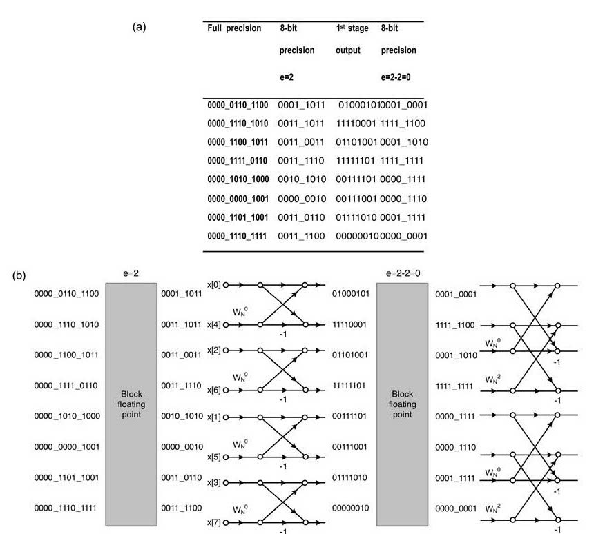
Block floating-point format is effectively used in computing the fast Fourier transform (FFT), where each butterfly stage processes a block of fixed-point numbers. Before these numbers are fed to the next stage, a block exponent is computed and then the intermediate result is truncated to be fed to the next block. Every stage of the FFT causes bit growth, but the block floating-point implementation can also cater for this growth.
Figure 3.22 Applying block floating-point format on data input in blocks to an algorithm
The first two stages of the Radix-2 FFT algorithm incur a growth by a factor of two. Before feeding the data to these stages, two redundant sign bits are left in the representation to accommodate this growth. The block floating-point computation, while scaling the data, keeps this factor in mind. For the remainder of the stages in the FFT algorithm, a bit growth by a factor off our is expected. For this, three redundant sign bits are left in the block floating-point implementation. The number of shifts these blocks of data go through from the first stage to the last is accumulated by adding the block exponent of each stage. The output values are then readjusted by a right shift by this amount to get the correct values, if required. The block floating point format improves precision as more valid bits take part in computation.
Figures 3.23(a) and (b) illustrate the first stage of a block floating-point implementation of an 8-point radix-2 FFT algorithm that caters for the potential of bit growth across the stages. While observing the minimum redundant sign bits (four in the figure) and keeping in consideration the bit growth in the first stage, the block of data is moved to the left by a factor of two and then converted to the requisite 8-bit precision. This makes the block exponent of the input stage to be 2. The output of the first stage in 8-bit precision is shown. Keeping in consideration the potential bit growth in the second stage, the block is shifted to the right by a factor of two. This shift makes the block exponent equal to zero. Not shown in the figure are the rest of the stages where the algorithm caters for bit growth and also observes the redundant sign bits to keep adjusting the block floating-point exponent.
3.8 Forms of Digital Filter
This section briefly describes different forms of FIR and IIR digital filters.
3.8.1 Infinite Impulse Response Filter
The transfer function and its corresponding difference equation for an IIR filter are given in (3.12) and (3.13), respectively:
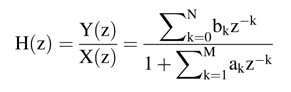
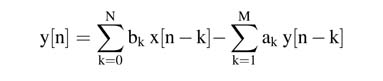
Figure 3.23 FFT butterfly structure employing block floating-point computation while keeping the bit growth issue in perspective
There are several mathematical ways of implementing the difference equation. The differences between these implementations can be observed if they are drawn as dataflow graphs (DFGs).Figure 3.24 draws these analytically equivalent DFGs for implementing N th-order IIR filter.
Although all these implementations are analytically equivalent, they do vary in terms of hardware resource requirements and their sensitivity to coefficient quantization. While implementing a signal processing algorithm in double- precision floating-point format, these varying forms have little practical significance; but for fixed-point implementation, it is important to understand their relative susceptibilities to quantization noise. It is important for a digital designer to understand that just converting a floating-point implementation to fixed-point using any optimization technique of choice may not yield desirable results and the system may even become unstable. It is therefore essential always to select a form that has minimum sensitivity to coefficient quantization before the format conversion is performed. Thus the first design objective for a fixed-point implementation of an algorithm is to choose a form that is least sensitive to quantization noise; and then, subsequent to this, the designer should try to minimize HW resources for the selected implementation.
3.8.2 Quantization of IIR Filter Coefficients
Fixed-point conversion of double-precision floating-point coefficients of an IIR filter moves the pole-zero location and thus affects the stability and frequency response of the system. To illustrate this effect, consider the design of an eighth-order system in MATLAB®, with pass-band ripple of 0.5 dB, stop-band attenuation of 50 dB and normalized cutoff frequency ω c = 0.15. The coefficients of the numerator b and denominator a obtained using MATLAB® function ellip with these specifications are given below:
b = 0.0046—0.0249 0.0655—0.1096 0.1289—0.1096 0.0655—0.0249 0.0046
a = 1.0000—6.9350 21.5565—39.1515 45.3884—34.3665 16.5896—4.6673 0.5860
The maximum values of the magnitude of the coefficients in b and a are 0.1289 and 45.3884, respectively. When converting the coefficients to fixed-point format, these values require an integer part of 1 and 7 bits, respectively. The word length of the fractional part is application-dependent.
Before any attempt is made to choose appropriate Q-formats for filter implementation, let us observe the effect of quantization on stability and frequency response of the system. The pole-zero plot of the filter transfer function with coefficients in double-precision floating-point numbers is shown in the top left part of Figure 3.25. Now the filter coefficients in arrays b and a are quantized to 24-bit, 16-bit and 12-bit precisions, and the Q-formats of these precisions are Q1.23 and Q7.17, Q1.15 and Q7.9, and Q1.11 and Q7.6, respectively. The pole-zero and the frequency response of the system for all these four cases are plotted in Figures 3.26 and 3.27, respectively.
It is evident from the pole-zero plots that the filter is unstable for 16-bit and 12-bit quantization cases as some of its poles move outside the unit circle. If an IIR filter is meant for fixed-point implementation, it is important to first select an appropriate form for the implementation before coding the design in high-level languages for its subsequent conversion to fixed-point format. The same filter has been implemented using second-order-sections (SoS), and pole-zero plots show that the filter is stable for all the above cases as all its poles remain inside the unit circle
Figure 3.24 Equivalent implementation for realizing an Nth-order IIR system. (a) Direct Form-I. (b) Direct Form-II. (c) Transposed Direct Form II. (d) Cascade form using DF-II second-order sections. (e) Parallel form using DF-II second-order sections
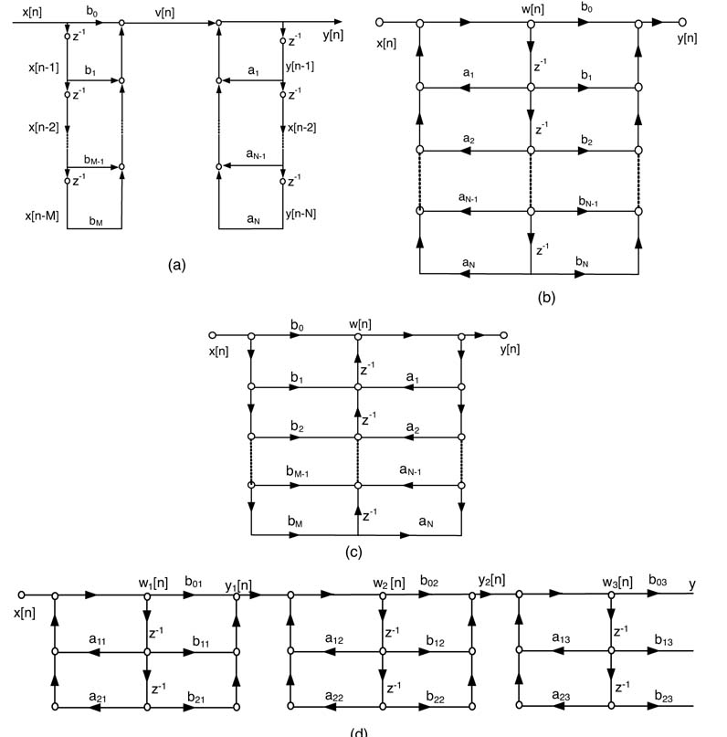
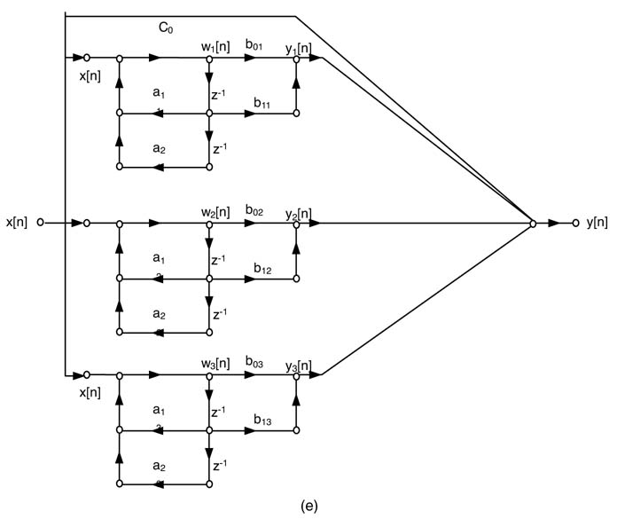
The matrix of coefficients for all the four sections from MATLAB® is:
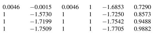
Each row lists three coefficients of b and three coefficients of a for its respective section. Based on the maximum of absolute values of the coefficients for each section, 2 bits are required for the integer part of respective Q-format. The filter is analyzed for 12-bit and 8-bit precision, and all the coefficients are converted into Q2.10 and Q2.6 format for the two formats. The pole-zero plots for these four sections for both the cases are shown in Figure 3.27. In both cases the designs using cascaded SoS are stable, so the overall system remains stable even for 8-bit quantization. It is therefore important to first analyze the stability of the system while selecting the word lengths for fixed-point implementation of IIR filters.
Figure 3.25 Effect of coefficient quantization on stability of the system. The system is unstable for 16-bit and 12-bit quantization as some of its poles are outside the unit circle
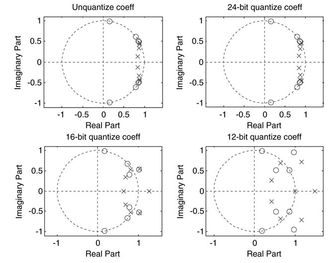
Figure 3.26 Frequency response of the eighth-order system for different quantization levels
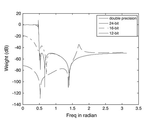
Figure 3.27 (a) Filter using cascaded SoSs with coefficients quantized in Q2.10 format. (b) Filter using cascaded SoSs with coefficients quantized in Q2.6 format
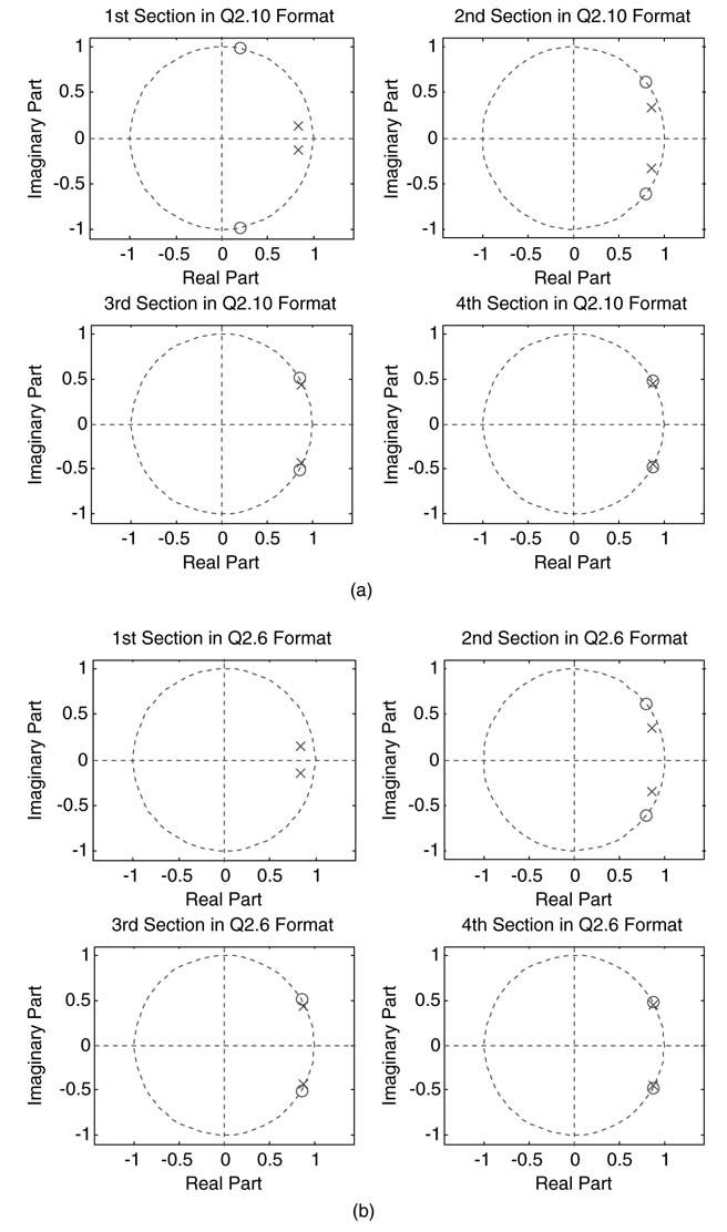
The filter in cascaded form can be designed with MATLAB®, first creating a filter design object:
>> d = fdesign.lowpass(’n,fp,ap,ast’,8,.15,.5,50)
d =
ResponseType:’Lowpass with passband-edge specifications and
 stopband attenuation’
SpecificationType:’N,Fp,Ap,Ast’
Description: {4x1 cell}
NormalizedFrequency: true
Fs:’Normalized’
FilterOrder: 8
Fpass: 0.1500
Apass: 0.5000
Astop: 50
Then design an elliptical filter on these specifications and automatically invoking MATLAB® filter visualization toolbox fvtool :
>> ellip(d); % Automatically starts fvtool to display the filter in second order sections.
By using a handle, all attributes of the filter can be displayed and changed according to requirements:
>> hd=ellip(d)
hd =
FilterStructure:’Direct-Form II, Second-Order Sections’
Arithmetic:’double’
sosMatrix: [4x6 double]
ScaleValues: [5x1 double]
ResetBeforeFiltering:’on’
States: [2x4 double]
NumSamplesProcessed: 0
Now the arithmetic precision of the coefficients can be changed to fixed-point by:
>> set(hd,’arithmetic’,’fixed’)
>> hd
hd =
FilterStructure:’Direct-Form II, Second-Order Sections’
Arithmetic:’fixed’
sosMatrix: [4x6 double]
ScaleValues: [5x1 double]
ResetBeforeFiltering:’on’
States: [2x4 embedded.fi]
NumSamplesProcessed: 0
CoeffWordLength: 16
CoeffAutoScale: true
Signed: true
InputWordLength: 16
InputFracLength: 15
StageInputWordLength: 16
StageInputAutoScale: true
StageOutputWordLength: 16
StageOutputAutoScale: true
OutputWordLength: 16
OutputMode:’AvoidOverflow’
StateWordLength: 16
StateFracLength: 15
ProductMode:’FullPrecision’
AccumMode:’KeepMSB’
AccumWordLength: 40
CastBeforeSum: true
RoundMode:’convergent’
OverflowMode:’wrap’
While exploring different design options for optimal word length, any of the attributes of hd can be changed using set directive.
Filter Design and Analysis Tool (FDATOOL) is a collection of tools for design, analysis, conversion and code generation. The tool designs FIR and IIR digital filters in both floating-point and fixed-point formats. The tool provides a great degree of control with a user-friendly interface. Figure 3.28 shows two snapshots of the GUI depicting all the design options available to the designer for designing, analyzing, fixed-point conversion and code generation. The elliptical filter can also be conveniently designed by setting different options in FDATOOL.
3.8.3 Coefficient Quantization Analysis of a Second-order Section
Even in second-order section the quantization effects can be further mitigated. The conversion in fixed-point format of the denominator coefficient as given in (3.14) creates a non-uniform grid:
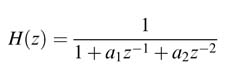
The grid is shown in Figure 3.29 for a 1 and a 2 converted to Q3.3 and Q2.4 formats, respectively. A filter design package, depending on the specifications, may place a double-precision pole at any point inside the unit circle. The conversion of the coefficients to fixed-point format moves the respective poles to quantized locations and makes the system experience more quantization noise at places with wider gaps. The structure given in Figure 3.30 creates a uniform rectangular grid and helps the designer to exactly model the quantization noise independent of location of its double-precision poles and zeros (r and θ are the radius and angle of the complex conjugate poles).
Figure 3.28 The MATLAB_ filter design and analysis toolbox offers varying options to design,quantize, analyze and generate Verilog or C code of a designed filter according to the given specifications
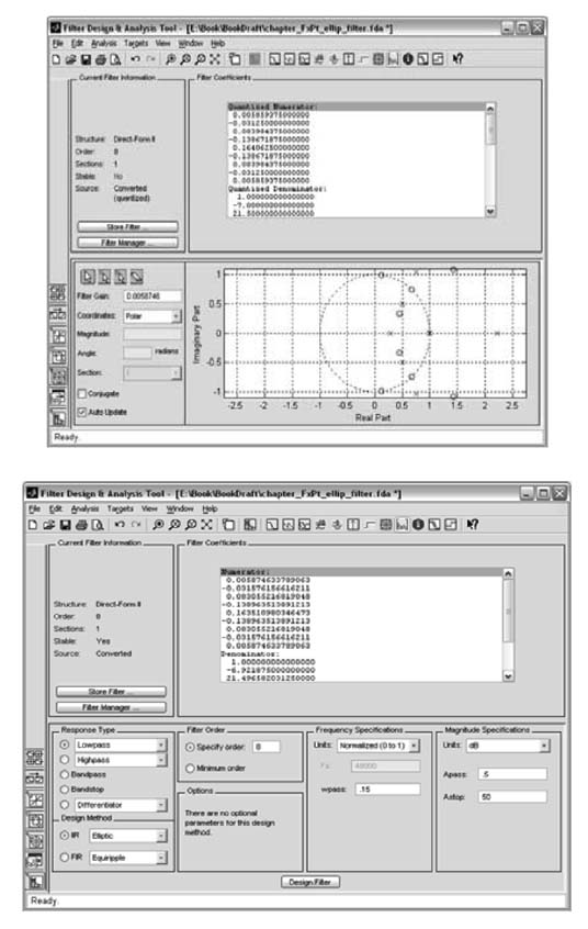
Figure 3.29 Possible pole locations when the coefficients of the denominator of an SoS are quantized to 6-bit fixed-point numbers
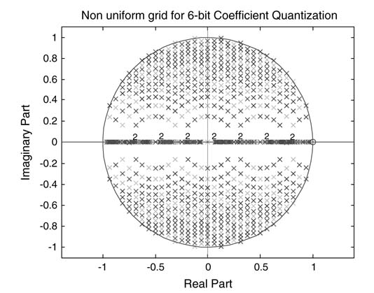
Figure 3.30 Filter structure to place quantized pole-pair re±jθ at intersections of evenly placed horizontal and vertical lines inside the unit circle
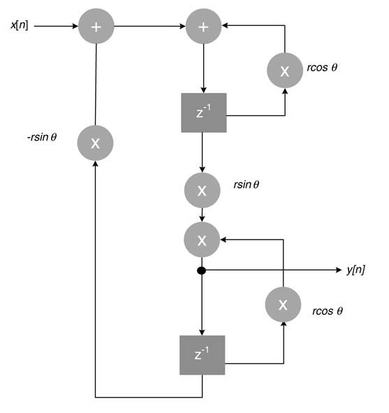
3.8.4 Folded FIR Filters
From the hardware perspective, a multiplier takes more area than an adder. FIR filter design using the MATLAB® filter design tool are symmetric or anti-symmetric and mathematically can be represented as:
This characteristic of the FIR filter can be effectively used to reduce the number of multipliers in mapping these designs in HW. The design can be folded to use this symmetry. For example, if the filter has four symmetric coefficients then convolution summation is written as:
The terms in this summation can be regrouped to reduce the number of multiplications from four to two. The new summation is:
The generalized folded flow graph that uses symmetry of the coefficients in an FIR is shown in Figure 3.31 for even and odd number of coefficients.
Figure 3.31 Symmetry of coefficients reduces the number of multipliers to almost half. (a) Folded design with odd number of coefficients. (b) Folded design with even number of coefficients
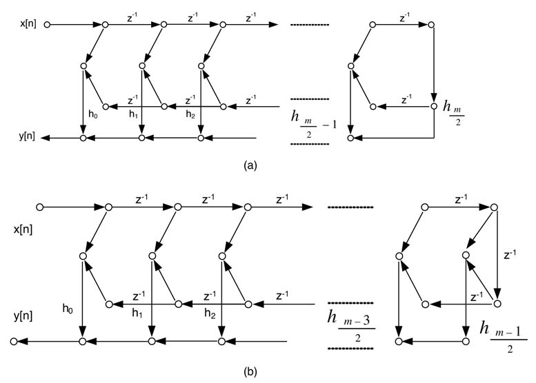
3.8.5 Coefficient Quantization of an FIR Filter
As FIR systems are always stable, stability is not a concern when quantizing double-precision floating-point coefficients of an FIR system to any fixed-point format. The coefficient quantization primarily adds an undesirable additional frequency response into the frequency response of the original system with double-precision floating-point coefficients. The mathematical reasoning of this addition is given in these expressions:
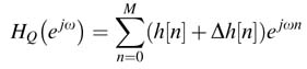
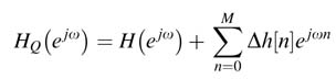
Thus quantization of coefficients of an FIR filter adds a frequency response equal to the frequency response of Δh[n] caused due to dropping of bits of h[n]. Consider a filter designed in MATLAB® using:
>> h=fir1(10,.1);
The coefficients are converted to Q1.7 format using the fi utility as:
>>hQ=fi(h, 1, 8,7);
Δh[n] is computed as:
>> hQ-h
and the respective values of these variables are:
h = 0.0100 0.0249 0.0668 0.1249 0.1756 0.1957 0.1756 0.1249 0.0668 0.0249 0.0100
h Q = 0.0078 0.0234 0.0703 0.1250 0.1719 0.1953 0.1719 0.1250 0.0703 0.0234 0.0078
Δh[n] = -0.0022 -0.0014
0.0035 0.0001 —0.0037 —0.0004 —0.0037 0.0001 0.0035 —0.0014 —0.0022
The quantization of coefficients obviously changes the frequency response of the filter. There is a possibility that the quantized filter may no longer satisfy the original design specifications. Figure 3.32 shows the original filter and modified filter, clearly demonstrating degradation in the pass-band ripples. The designer may need to over-design a filter to let the quantization effects use this leverage for meeting the specifications.
A more optimal solution to this problem is to design a filter in the fixed-point domain. Researchers have tended to focus more on conversion of signal processing applications originally designed using floating-point format to fixed-point implementation, but very few have investigated designing in the fixed-point format. A direct design in fixed-point gives more control to the designer and takes his or her worry away from meeting a specification while finding an optimal word length for the coefficients. These techniques take the system specification and then directly design the system in fixed-point format. Optimization techniques are exploited, but these techniques have yet not found a place in commercial toolboxes primarily because of their computational complexity. Finding computationally feasible techniques requires more deliberation and effort from researchers working in areas of signal processing and digital design.
Figure 3.32 Change in magnitude of frequency response due to floating-point to fixed-point conversion
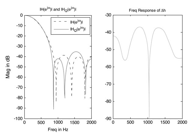
Exercises
Exercise 3.1
Design a 13-bit floating-point multiplier. The floating-point number has 1, 4 and 8 bits for, respectively, its sign s, exponential e and mantissa m. Assume a bias value of 7 for the representation. Use an 8 x 8-bit unsigned multiplier to multiply two mantissas, and a 4-bit adder and a subtractor to add the two exponents and then subtract the bias to take the effect of twice added bias from the addition. Normalize the multiplication and add its effect in the computed exponential. Draw an RTL diagram and code the design in Verilog. Write a stimulus to check your design for normalized and denormalized values. Finally, check the design for multiplication by ±∞.
Exercise 3.2
Add the following two floating-point numbers using 32-bit IEEE floating-point format. Show all the steps in the addition that should help in designing a floating-point adder. The numbers are:
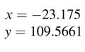
Exercise 3.3
Design a floating-point multiply accumulator (MAC) that first multiplies two 32-bit numbers and then adds the accumulator into the product. The MAC unit should only normalize the result once after multiplication and addition. Code the design in RTL and write a stimulus to test the design.
Exercise 3.4
Convert the floating-point implementation of Section 3.2.3 to 16-bit fixed-point format. Simulate the floating point and fixed-point implementation. Design a receiver that demodulates the signal. Count bit errors. Add AWGN (additive white Gaussian noise) and count bit errors for different signal-to-noise ratios.
Exercise 3.5
Multiply the following 8-bit numbers A and B by considering them as U × U, U × S, S × U and S × S, where U and S stands for unsigned and signed fraction numbers:
A = 8'b 1011_0011
B = 8'b 1100_0101
Also multiply the numbers considering both of these numbers as signed integers and then signed fractional numbers in Q1.7 format. Also multiply them by considering A as a signed integer and B as a signed Q1.7 format number. Design the HW and implement it in RTL Verilog.
Exercise 3.6
Add rounding and truncation logic in the 17 × 17-bit unified multiplier of Figure 3.18. The design should generate a 16-bit product and also generate a flag if truncation of the integer multiplication results in overflow.
Exercise 3.7
Design HW logic to implement a block floating-point module that computes a block exponential of an 8-element 16-bit array of numbers before truncating them to 8-bit numbers. Test your design for multiple blocks of data with a block exponent varying from 0 to 7. Realize the design in RTL Verilog.
Exercise 3.8
Floating-point implementation of a component of a communication algorithm is given below:
double Mixer_Out[3];
double Buff_Delayline[3];
// Filter coefficients in double precision
double HF_DEN [] = {1.0000, -1.0275, 0.7265};
double HF_NUM [] = {0.1367, 0.5, -0.1367};
// Input values for testing the code
#define LEN_INPUT 10
double input[LEN_INPUT] = {
 0.2251, 0.4273, 0.6430, 0.8349, 1.0089, 0.6788, 0.3610,
 -0.3400, -0.6385, -0.8867};
// Section of the code for floating to fixed-point conversion, the code to be written in a function for simulation
for(int i=0; i<LEN_INPUT; i++)
{
 Mixer_Out[2] =Mixer_Out[1];
 Mixer_Out[1] =Mixer_Out[0];
 Mixer_Out[0] =input[i];
 Buff_Delayline[2] = Buff_Delayline[1];
 Buff_Delayline[1] = Buff_Delayline[0];
 Buff_Delayline[0]=-Buff_Delayline[1]*HF_DEN[1]
 -Buff_Delayline[2]*HF_DEN[2]
 +Mixer_Out[0]*HF_NUM[0]
 +Mixer_Out[1]*HF_NUM[1]
 +Mixer_Out[2] * HF_NUM[2];
}
1. Simulate the communication algorithm using input samples from the floating-point array input[] .
2. Convert the algorithm into fixed-point format using 16-bit precision by appropriately converting all the variables into Qn.m format, where n + m = 16.
3. Compare your fixed-point result with the floating-point implementation for the same set of inputs in fixed-point format.
4. Draw RTL design of computations that are performed in the loop.
Exercise 3.9
To implement the difference equation below in fixed-point hardware, assume the input and output are in Q1.7 format:
First convert the coefficients to appropriate 8-bit fixed-point format, use rounding followed by truncation and saturation logic. Simulate the floating-point and fixed-point implementation in MATLAB®. Code the design in RTL Verilog. Write stimulus and compare the results with the MATLAB® simulation result.
Exercise 3.10
Implement the following equation, where x[n] and y[n] are in Q1.7 and Q2.6 formats, respectively, and z[n] is an unsigned number in Q0.8 format. Design architecture for computing:
Give the Q format of w [n ].
Exercise 3.11
The C code below implements this difference equation for 12 input values y[n] = – 2.375x [n ] + 1.24y[n– 1]:
aty[12], x[12];
y[0] =0.0
for (n =1; n< 12; n++)
{
y[n] = -2.375 x[n] +1.24 y[n-1];
}
The code defines floating-point arrays x [.] and y [.]. Convert the code to appropriate fixed-point format. Specify the format and simulate the implementation for given values of input. Assume |x [n ]| < 1. Compare your result with the floating-point implementation result. Calculate the mean squared error by computing the mean of squares of differences of the two output values for the test vector given below:

Exercise 3.12
Write RTL Verilog code to implement a four-coefficient FIR filter given in Figure 3.33. Assume all the coefficients h0 .. .h 3 and input datax [n ]are in Q1.15 format. Appropriately truncate the result from multiplication units to use 18-bit adders, and define the appropriate format for y [n ].Optimize the design assuming the coefficients of the FIR filter are symmetric.
Exercise 3.13
Using the MATLAB® filter toolbox, design an IIR filter with the following specifications: δ1 = 0.001; δ2 = 0.0001; wp = 0.2π; ws = 0.25π. Convert the filter into multiple cascaded second-order sections, and then quantize the coefficients as 16-bit signed numbers using an appropriate Qn.m format. Draw the dataflow of the design and write RTL Verilog code to implement the design using signed arithmetic.
Figure 3.33 Four-coefficient FIR filter
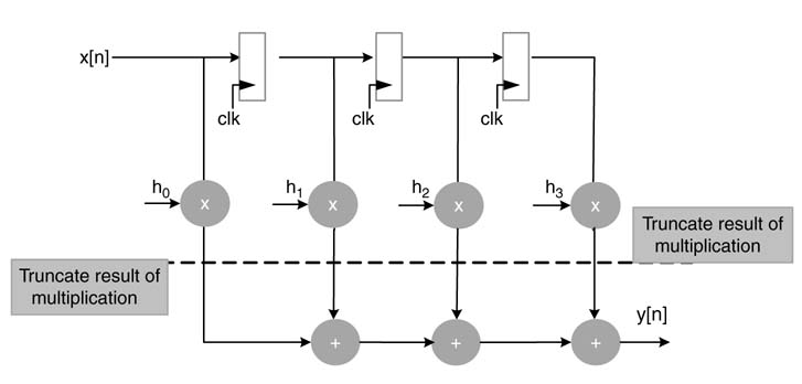
References
1. www.altera.com/products/software/products/dsp/dsp-builder.xhtml
2. www.xilinx.com/tools/sysgen.htm
3. J. J. F. Cavanagh, Digital Computer Arithmetic , 1984, McGraw-Hill.
4. V. C. Hamachar, Z. G. Vranesic and S. G. Zaky, Computer Organization , 1990, McGraw-Hill.
5. M. M. Mano, Computer Engineering , 1988, Prentice-Hall.
6. J. F. Wakerly, Digital Design Principles und Practices , 1990, Prentice-Hall.
7. S. Waserand M. J. Flynn, Introduction to Arithmetic for Digital Systems Designers , 1982, Holt, Rinehart & Winston.
8. R. C. Dorf, Computers, Software Engineering, and Digital Devices , 2005, CRC Press.
9. ANSI/IEEE, Standard 754-1985: “Binary floating-point arithmetic,” 1985.
10. P. Karlstr€om, A. Ehliarand D. Liu, “High-performance low-latency FPGA-based floating-point adder and multiplier units in a Virtex 4,” in Proceedings of the 24th Norchip Conference , 2006, pp. 31–34, Linkoping, Sweden.
11. G. Govindu, L. Zhuo, S. Choi, P. Gundalaand V. K. Prasanna,“Area and power performance analysis of a floatingpoint based application on FPGAs,” in Proceedings of the 7th Annual Workshop on High-performance Embedded Computing , 2003, Lincoln Laboratory, MIT, USA.
12. K. Han and B. L. Evans, “Optimum word-length search using a complexity-and-distortion measure,” EURASIP Journal of Applied Signal Processes , 2006, no. 5, pp. 103–116.