
Chapter 5. Statement Refactoring
The problem for us was to move forward to a decisive victory, or our cause was lost.
—Ulysses S. Grant (1822–1885)
Personal Memoirs, Chapter XXXVII
EVEN IF THERE IS OFTEN STILL ROOM FOR IMPROVEMENT WHEN ALL QUERIES HAVE BEEN “TUNED TO death,” as you saw in Chapter 1 (and as I will further demonstrate in the next few chapters), when a big, bad query flagrantly kills performance, improving that query has a tremendous psychological effect. If you want to be viewed with awe, it is usually better to improve a killer query than to humbly ensure that the system will be able to scale up in the next few months.
Although optimizers are supposed to turn a poorly expressed statement into efficient data handling, sometimes things go wrong, even when the indexing is sane and all the relevant information is available to the optimizer. You know how it is: even if the optimizer does a good job 99 times out of 100, it is the botched attempt that everyone will notice. Assuming once again that proper statistics are available to the optimizer, failure to perform well usually results from one of the following:
An optimizer bug (it happens!)
A query that is so complex that the optimizer tried, in the limited time it grants itself, only a small number of rewrites compared to the large number of possible combinations, and failed to find the best path in the process
I’d like to point out that optimizer bugs are most commonly encountered in situations of almost inextricable complexity, and that properly writing the query is the most efficient workaround. Very often, writing a query in a simpler, more straightforward way requires much less work from the optimizer that will “hit” a good, efficient execution path faster. In fact, writing SQL well is a skill that you can compare to writing well: if you express yourself badly, chances are you will be misunderstood. Similarly, if you just patch together joins, where conditions, and subqueries, the optimizer may lose track of what is really critical in identifying the result set you ultimately want, and will embark on the wrong route.
Because what most people define as a "slow statement” is actually a statement that retrieves rows more slowly than expected, we could say that a slow statement is a statement with an “underperforming where clause.” Several SQL statements can take a where clause. For most of this chapter, I will refer to select statements, with the understanding that the where clauses of update and delete statements, which also need to retrieve rows, follow the same rules.
Execution Plans and Optimizer Directives
First, a word of warning: many people link query rewriting to the analysis of execution plans. I don’t. There will be no execution plan in what follows, which some people may find so strange that I feel the need to apologize about it. I can read an execution plan, but it doesn’t say much to me. An execution plan just tells what has happened or will happen. It isn’t bad or good in itself. What gives value to your understanding of an execution plan is an implicit comparison with what you think would be a better execution plan: for instance, “It would probably run faster if it were using this index; why is it doing a full table scan?” Perhaps some people just think in terms of execution plans. I find it much easier to think in terms of queries. The execution plan of a complex query can run for pages and pages; I have also seen the text of some queries running for pages and pages, but as a general rule a query is shorter than its execution plan, and for me it is far more understandable. In truth, whenever I read a query I more or less confusedly “see” what the SQL engine will probably try to do, which can be considered a very special sort of execution plan. But I have never learned anything really useful from the analysis of an execution plan that execution time, a careful reading of statements, and a couple of queries against the data dictionary didn’t tell me as clearly.
I find that execution plans are as helpful as super-detailed driving instructions, such as “drive for 427 meters/yards/whatever, and then turn left into Route 96 and drive for 2.23 kilometers/miles/whatever….” If I don’t know where I’m going, as soon as I miss an exit I will be lost. I’m much more comfortable with visual clues that I can identify easily, such as a gas station, a restaurant, or any other type of landmark, than with precise distances computed from maps, and road numbers or street names that are not always easy to read when you are driving. My approach to SQL is very similar; my landmarks are the knowledge of which tables are really big tables, which criteria are really selective, and where the reliable indexes are. An SQL statement tells a story, has a kind of plot; like a journey, you start from point A (the filtering conditions you find in your where clause), and you are going to point B (the result set you want). When you drive and find that it took far too long to get from point A to point B, a detailed analysis of the road you took will not necessarily help you to determine why the trip took so long. Counting traffic lights and timing how long you waited at each light may be more useful in explaining why it took so much time, but it will not tell you, the driver, what is the best route. A methodical study of traffic conditions is highly valuable to city planners, who look for places where congestion occurs and try to remove black spots. From my selfish point of view as a driver, in my quest for a faster way to get from point A to point B, I just need to know the places I’d rather avoid, study the map, and rethink my journey. Similarly, I find certain tuning approaches to be more appropriate for DBAs than for developers, simply because each group can pull different levers. You may or may not share my views; we have different sensibilities, and we may feel more comfortable with one approach than with another. Anyway, very often, different approaches converge toward the same point, although not always at the same speed. This chapter describes statement rewriting as I see and practice it.
If the way you approach a query and the way you achieve a faster query leaves much latitude to personal taste, I have many more qualms with optimizer directives (or hints), which some people consider the ultimate weapon in tuning efforts. Optimizer directives work; I have used them before and will probably use them again. Arguably, in some cases a directive makes for more maintainable code than an SQL trick to the same effect. Nevertheless, I consider the use of directives to be a questionable practice that is better avoided, and whenever I have to resort to them I feel like laying down my weapons and surrendering.
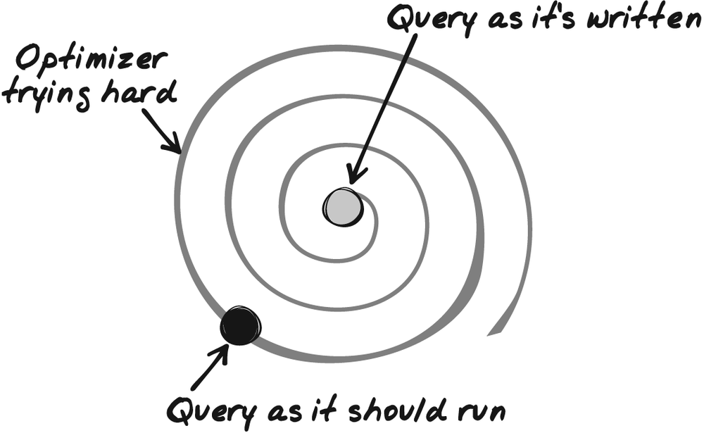
I will now explain with a few figures why I have such a dislike of optimizer directives. SQL is supposed to be a declarative language; in other words, you are supposed to state what you want and not how the database should get it. All the same, when you have a query you can consider that there is a “natural way” to execute it. This “natural way” is dictated by the way the query is written. For instance, if you have the following from clause:
from table1
inner join table2
on ...
inner join table3
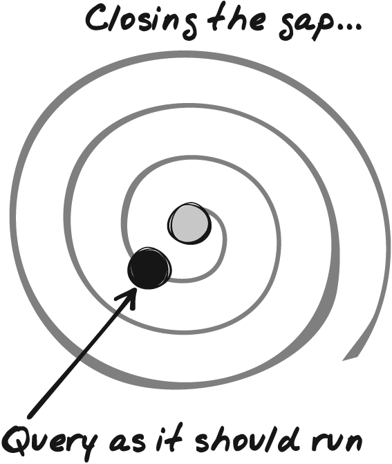
on ...you may consider that the natural way is to search table1 first for whatever is needed, then table2, then table3, using conditions expressed in the where clause to link the tables in a kind of chain. Of course, this would be a very naive approach to query execution. The task of the query optimizer is to check the various conditions and estimate how effectively they filter the data and how effectively they allow fast funneling on the final result. The optimizer will try to decide whether starting with table2, then proceeding to table3, then to table1 or any other combination would not be more efficient; similarly, it will decide whether using an index will be beneficial or detrimental. After pondering a number of possibilities, the optimizer will settle for an execution plan corresponding to the “natural way” of executing a functionally equivalent but different query. Figure 5-1 shows my representation of the work of the optimizer and how it transforms the original query into something different.
The difficulties of the optimizer are twofold. First, it is allotted a limited amount of time to perform its work, and in the case of a complex query, it cannot try all possible combinations or rewritings. For example, with Oracle, the optimizer_max_permutations parameter determines a maximum number of combinations to try. At some point, the optimizer will give up, and may decide to execute a deeply nested subquery as is, instead of trying to be smart, because it lacks the time to refine its analysis. Second, the more complex the query, the less precise the cost estimates that the optimizer compares. When the optimizer considers the different steps it might take, a crucial element is how much each step contributes to refining the result and how much it helps to focus on the final result set—that is, if I have that many rows in input, how many rows will I get as output? Even when you use a primary or unique key in a query to fetch data, there is a little uncertainty about the outcome: you may get one row, or none. Of course, the situation is worse when the criteria can match many rows. Every cost that the optimizer estimates is precisely that, an estimate. When the query is very complicated, errors in estimates cascade, sometimes canceling one another, sometimes accumulating. The optimizer increases the risk of having its estimates wrong.
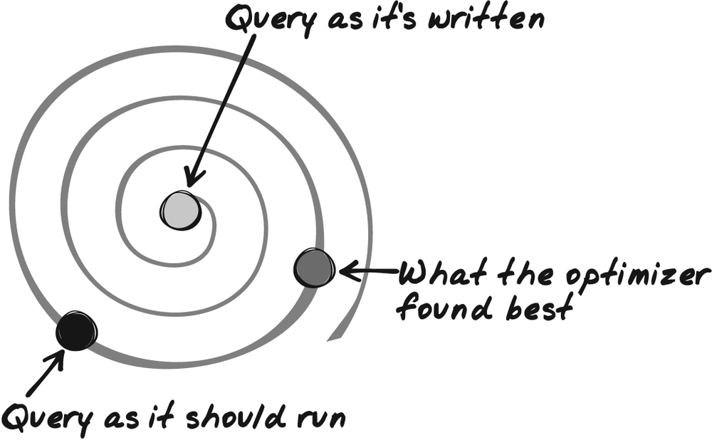
As a result, when a complex query is very poorly written, the optimizer will often be unable to close the gap and find the best equivalent query. What will happen is a situation such as that shown in Figure 5-2: the optimizer will settle for an equivalent query that according to its estimates is better than the original one but perhaps only marginally so, and will miss an execution plan that would have been much faster.
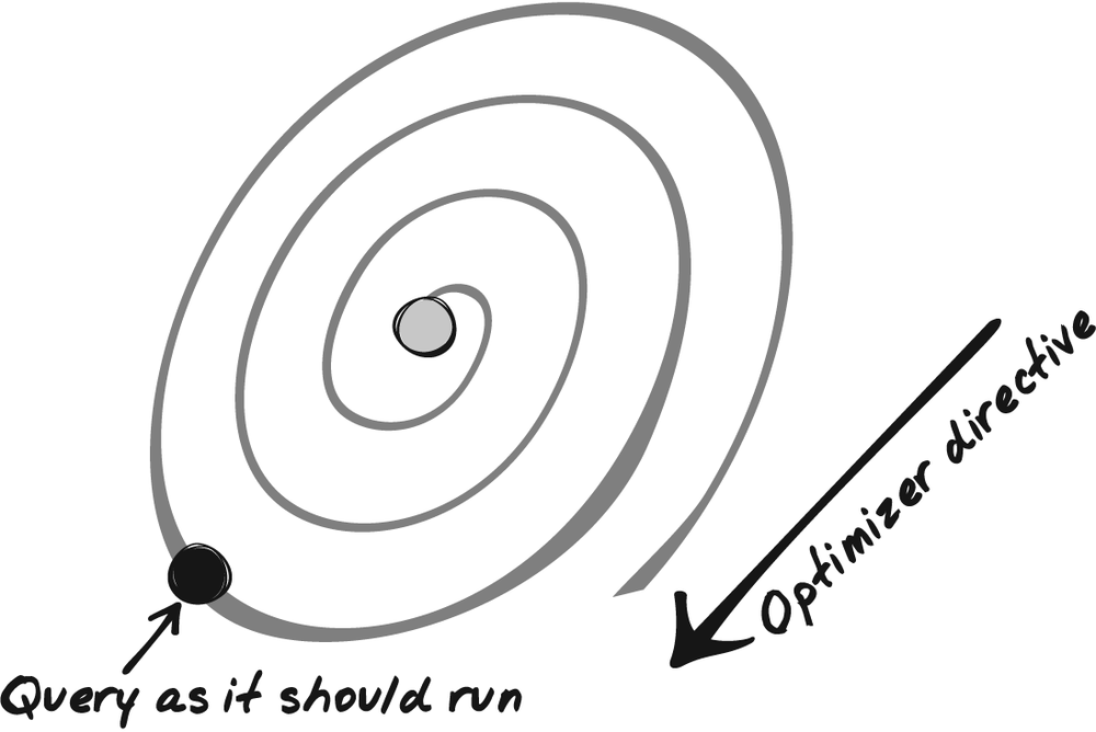
In such a case, many people fall back on optimizer directives; having some idea about what the execution plan should be (possibly because they got it in a different environment, or prior to a software update, or because they stumbled upon it trying a number of directives), they add to the query DBMS-specific directives that orient the efforts of the optimizer in one direction, as shown in Figure 5-3.
The systematic use of directives is also applied when you try to achieve plan stability, the possibility offered by some products to record an execution plan that is deemed satisfactory and replay it whenever the same query is executed again.
My issue with directives and plan stability is that we are not living in a static world. As Heraclitus remarked 2,500 years ago, you never step into the same river twice: it’s no longer the same water, nor the same human being. Put in a business perspective, the number of customers of your company may have changed a lot between last year and this year; last year’s cash-cow product may be on the wane, while something hardly out of the labs may have been an instant success. One of the goals of optimizers is to adapt execution plans to changing conditions, whether it is in terms of volume of data, distribution of data, or even machine load. Going back to my driving analogy, you may take a different route to get to the same place depending on whether you left at rush hour or at a quieter time.
If you cast execution plans in stone, unless it is a temporary measure, sooner or later the situation shown in Figure 5-4 will occur: what once was the best execution plan no longer will be, and the straightjacketed optimizer will be unable to pull out the proper execution path.
Even in a stable business environment, you may have bad surprises: optimizers are a dynamic part of DBMS products, and even if you rarely see optimizers mentioned in marketing blurbs, they evolve significantly between versions to support new features and to correct quirks. Directives may be interpreted slightly differently. As a result, some major software upgrades may become nightmarish with applications that intensively use optimizer directives.
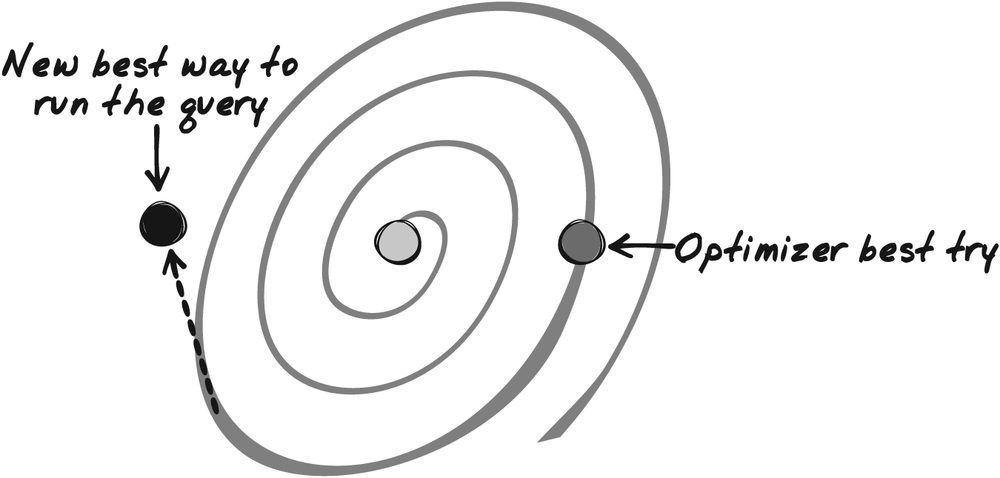
I hope you understand the reasons behind my uneasiness with optimizer directives; my goal when I rewrite a query is to turn the optimizer into my ally, not to prove that I am smarter than it is. My aim, therefore, is to rewrite a query in a simpler fashion that will not “lose” the optimizer, and to move, as in Figure 5-5, as closely as I can to what I estimate to be, under the present circumstances, the best writing of the query. For me, the best writing of the query is what best matches what the SQL engine should do. It may not be the “absolute best” writing, and over time the fastest execution plan may drift away from what I wrote. But then, the optimizer will be able to play its role and keep stable performance, not stable execution plans.
Now that I have expressed my goal, let’s see how I can achieve it.
Analyzing a Slow Query
The first thing to do before analyzing a slow query is to bravely brace yourself against what may look like an extraordinarily complex statement. Very often, if you resist the temptation of running away screaming, you will have half won already. If indexing is reasonable, if statistics are up-to-date, and if the optimizer got lost, chances are that the statement is ugly (if it doesn’t look ugly, its ugliness is probably hidden deep inside a view or user-written function). If the query refers to one or several views, it is probably best to find the text of the views and to reinject it inside the query as subqueries (this can be a recursive process). It will not make the query look better, but you will have a global view, and actually, it is often easier to analyze a daunting SQL statement than a mishmash of procedural calls. After all, like beauty, complexity is in the eye of the beholder. The case of functions is somewhat more difficult to handle than the case of views, as you saw in the previous chapter. If the functions refer to tables that don’t appear in the query, it is probably better as a first stage to leave them in place, while keeping an eye on the number of times they may be called. If functions refer to tables already present in the query, and if their logic isn’t too complicated, it’s probably better to try to reinject them in the query, at least as an experiment.
Whenever I analyze a query, I always find that the most difficult part of the analysis is answering the question “what are the query writers trying to do?”
Getting help from someone who is both functionally knowledgeable and SQL-literate is immensely profitable, but there are many cases when you need to touch some very old part of the code that no one understands any longer, and you are on your own. If you want to understand something that is really complex, there aren’t tons of ways to do it: basically, you must break the query into more manageable chunks. The first step in this direction is to identify what really matters in the query.
Identifying the Query Core
When you are working on a complex query, it is important to try to pare the query down to its core. The core query involves the minimum number of columns and tables required to identify the final result set. Think of it as the skeleton of the query. The number of rows the core query returns must be identical to the number of rows returned by the query you are trying to improve; the number of columns the core query returns will probably be much smaller.
Often, you can classify the columns you need to handle into two distinct categories: core columns that are vital for identifying your result set (or the rows you want to act on), and "cosmetic” columns that return information directly derivable from the core columns. Core columns are to your query what primary key columns are to a table, but primary key columns are not necessarily core columns. Within a table, a column that is a core column for one query can become a cosmetic column in another query. For instance, if you want to display a customer name when you enter the customer code, the name is cosmetic and the code is the core column. But if you run a query in which the name is a selection criterion, the name becomes a core column and the customer code may be cosmetic if it isn’t involved in a join that further limits the result set. So, in summary, core columns are:
The columns to which filtering applies to define the result set
Plus the key columns (as in primary/foreign key) that allow you to join together tables to which the previous columns belong
Sometimes no column from the table from which you return data is a core column. For instance, look at the following query, where the finclsref column is the primary key of the tdsfincbhcls table:
select count(*),
       coalesce(sum(t1.boughtamount)
                - sum(t1.soldamount), 0)
from tdsfincbhcls t1,
     fincbhcls t2,
     finrdvcls t3
where t1.finclsref = t2.finclsref
  and t2.finstatus = 'MA'
  and t2.finpayable = 'Y'
  and t2.rdvcode = t3.rdvcode
  and t3.valdate = ?
  and t3.ratecode = ?
Although the query returns information from only the tdsfincbhcls table, also known as t1, what truly determines the result set is what happens on the t2/t3 front, because you need only t2 and t3 to get all the primary keys (from t1) that determine the result set. Indeed, if in the following query the subquery returns unique values (if it doesn’t, there is probably a bug in the original query anyway), we could alternatively write:
select count(*),
       coalesce(sum(t1.boughtamount)
                - sum(t1.soldamount), 0)
from tdsfincbhcls t1
where t1.finclsref in
       (select t2.finclsref
        from fincbhcls t2,
             finrdvcls t3
        where t2.finstatus = 'MA'
          and t2.finpayable = 'Y'
          and t2.rdvcode = t3.rdvcode
          and t3.valdate = ?
          and t3.ratecode = ?
          and t2.finclsref is not null)
The first step we must take when improving the query is to ensure that the subquery, which really is the core of the initial query, runs fast. We will need to consider the join afterward, but the speed of the subquery is a prerequisite to good performance.
Cleaning Up the from Clause
As the previous example shows, you should check the role of tables that appear in the from clause when you identify what really matters for shaping the result set. There are primarily three types of tables:
Tables from which data is returned, and to the columns of which some conditions (search criteria) may or may not be applied
Tables from which no data is returned, but to which conditions are applied; the criteria applied to tables of the second type become indirect conditions for the tables of the first type
Tables that appear only as “glue” between the two other types of tables, allowing us to link the tables that matter through joins
Figure 5-6 shows how a typical query might look with respect to the various types of tables involved. Tables are represented by rectangles, and the joins are shown as arrows. The data that is returned comes from tables A and D, but a condition is also applied to columns from table E. Finally, we have two tables, B and C, from which nothing is returned; their columns appear only in join conditions.
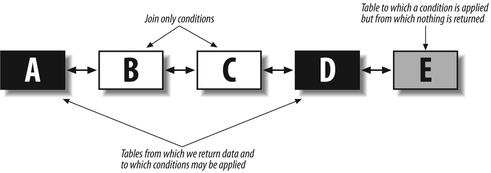
Therefore, we obtain a kind of chain of tables, linked to one another through joins. In some cases, we might have different branches. The tables to watch are those at the end of the branches. Let’s start with the easiest one, table E. Table E belongs to the query core, because a condition is applied to it (unless the condition is always true, which can happen sometimes). However, it doesn’t really belong to the from clause, because no data directly comes “from” table E. The purpose of table E is to provide an existence (or nonexistence) condition: the reference to table E expresses " . . . and we want those rows for which there exists a matching row in E that satisfies this condition.” The logical place to find a reference to table E is in a subquery.
There are several ways to write subqueries, and later in this chapter I will discuss the best way. We can also inject subqueries at various points in the main query, the select list, the from clause, and the where clause. At this stage, let’s keep the writing simple. Let me emphasize the fact that I am just trying to make the query more legible before speeding it up. I can take table E out of the from clause and instead write something like this:
and D.join_column in (select join_column from E where <conditions>)For table A, if the query both returns data from the table and applies search criteria to its columns, there is no doubt that it belongs to the query core.
However, we must study harder if some data is returned from table A but no particular search criterion is applied to it except join conditions. The fate of table A in such a case depends on the answer to two questions:
- Can the column from table
Bthat is used for the join be null? Null columns, the value of which is unknown, cannot be said to be equal to anything, not even another null column. If you remove the join between tables
AandB, a row from tableBwill belong to the result set if all other conditions are satisfied but the column involved in the join is null; if you keep the join, it will not belong to the result set. In other words, if the column from tableBcan be null, the join with tableAwill contribute to shape the result set and will be part of the query core.- If the column from table
Bthat is used for the join is mandatory, is the join an implicit existence test? To answer that question, you need to understand that a join may have one of two purposes:
To return associated data from another table, such as a join on a customer identifier to retrieve the customer’s name and address. This is typically a case of foreign key relationship. A name is always associated to a customer identifier. We just want to know which one (we want to know the cosmetic information). This type of join doesn’t belong to the query core.
To return data, but also to check that there is a matching row, with the implicit statement that in some cases no matching row will be found. An example could be to return order information for orders that are ready to be shipped. Such a join contributes to define the result set. In that case, we must keep the join inside the query core.
Distinguishing between joins that only provide data to adorn an already defined result set and joins that contribute to reducing that result set is one of the key steps in identifying what matters. In the process, you should take a hard look at any distinct clause that you encounter and challenge its usefulness; once you have consigned to subqueries tables that are present to implement existence conditions, you will realize that many distinct clauses can go, without any impact on the query result. Getting rid of a distinct clause isn’t simply a matter of having eight fewer characters to type: if I empty my purse in front of you and ask you how many distinct coins I have, the first thing you’ll do is to sort the coins, which will take some time. If I give you only distinct coins, you’ll be able to answer immediately.
Like you, an SQL engine needs to sort to eliminate duplicates; it takes CPU, memory, and time to do that.
Sometimes you may notice that during this cleaning process some of the joins are perfectly useless. [37] While writing this book, I was asked to audit the performance of an application that had already been audited twice for poor performance. Both previous audits had pointed at queries built on the following pattern that uses the Oracle-specific syntax (+) to indicate an outer join (the table that is outer-joined is the one on the (+) side). All of these queries were taking more than 30 seconds to run.
select count(paymentdetail.paymentdetailid)
from paymentdetail,
     payment,
     paymentgrp
where paymentdetail.paymentid = payment.paymentid (+)
and payment.paymentgrpid = paymentgrp.paymentgrpid (+)
and paymentdetail.alive = 'Y'
and paymentdetail.errorid = 0
and paymentdetail.mode in ('CARD', 'CHECK', 'TRANSFER')
and paymentdetail.payed_by like 'something%'
Recommendations included the usual mix of index creation and haphazard database parameter changes, plus, because all three “tables” in the from clause were actually views (simple unions), the advice to use materialized views instead. I was apparently the first one to spot that all criteria were applied to paymentdetail, and that the removal of both payment and paymentgrp from the query changed nothing to the result, except that the query was now running in three seconds (without any other change). I hurried to add that I didn’t believe that this counting of identifiers was of any real use anyway (more about this in Chapter 6).
At this early stage of query refactoring, I am just trying to simplify the query as much as I can, and return the most concise result I can; if I could, I’d return only primary key values. Working on a very lean query is particularly important when you have aggregates in your query—or when the shape of the query suggests that an aggregate such as the computation of minimum values would provide an elegant solution. The reason is that most aggregates imply sorts. If you sort on only the minimum number of columns required, the volume of data will be much smaller than if you sort on rows that are rich with information; you will be able to do much more in memory and use fewer resources, which will result in much faster processing.
After we have identified the skeleton and scraped off rococo embellishments, we can work on structural modifications.
Refactoring the Query Core
You must consider the query core that you have obtained as the focus of your efforts. However, a query that returns minimum information isn’t necessarily fast. This query is easier to work with, but you must rewrite it if it’s still too slow. Let’s study the various improvements you can bring to the query core to try to make it faster.
Unitary Analysis
A complex query is usually made of a combination of simpler queries: various select statements combined by set operators such as union, or subqueries. There may also be an implicit flow of these various simpler queries: some parts may need to be evaluated before others because of dependencies. It is worth noting that the optimizer may copyedit the SQL code, and in fact change or even reverse the order of dependencies. In some cases, the DBMS may even be able to split a query and execute some independent sections in parallel. But whatever happens, one thing is true: a big, slow query generally is a combination of smaller queries. Needless to say, the time required to execute the full query can never be shorter than the time that is required to execute the longest step.
You will often reach a good solution faster if you “profile” your query by checking the “strength” of the various criteria you provide. That will tell you precisely where you must act, and moreover, in the process it may indicate how much improvement you can expect.
Eliminating Repeated Patterns
It is now time to hunt down tables that are referenced several times. We can find a reference to the same table in numerous places:
In different sections of a query that uses set operators such as
unionIn subqueries at various places, such as the
selectlist,fromclause,whereclause, and so forthUnder various other guises in the
fromclause:— As a self-join—that is, a table directly linked to itself through different columns belonging to the same functional domain. An example could be a query that displays the manager’s name alongside the employee’s name when the employee ID of the manager is an attribute of the row that describes an employee.
— Through an intermediate table that establishes a link between two different rows of a given table; for instance, in a genealogical database the
marriagestable would establish a link between two different rows from thepersonstable.
When you have spotted a table that seems to appear with some insistence in a query, you need to ask yourself two questions, in this order:
Can I fetch all the data I need from this table in a single access to the table?
If I can get all the data in a single pass, is it worthwhile to do so?
To give you an example, I once encountered in a query the following condition, where x is an alias for a table in the from clause (not shown):
... and ((select min(o.hierlevel) from projvisibility p, org owhere p.projversion = x.versionand p.id = x.idand p.accessid = o.parentidand o.id = ?)= (select min(o.hierlevel) from projvisibility p, org owhere p.projversion = x.versionand p.id = x.idand p.accessid = o.parentidand o.id = ?and p.readallowed = 'Y'))
Here we have an obvious case of a repeated pattern, because after having verified that the two values that are substituted with the two ? place markers are indeed identical, we see that the only difference between the two subqueries is the last line in the preceding code snippet. What is this part of the query operating on? Basically, we are processing a set of values that is determined by three values, two of them inherited from the outer query (x.version and x.id), and the third one passed as a parameter. I will call this set of values S.
We are comparing a minimum value for S to the minimum value for a subset of S defined by the value Y for the readallowed column of the projvisibility table; let’s call the subset SR. When the SQL engine is going to examine S, looking for the minimum value, it will necessarily examine the values of SR at the same time. Therefore, the second subquery clearly appears as redundant work.
The magical SQL construct for comparing subsets within a set is often case. Collecting the two minimum values at once isn’t too difficult. All I have to do is to write:
select min(o.hierlevel)  absolute_min,
       min(case p.readallowed
             when 'Y' then o.hierlevel
             else null
           end) relative_min
from ...
null is ignored by a function such as min(), and I get my two values in a single pass. I just have to slightly modify the original query into the following:
... and exists (select null
                from projvisibility p,
                     org o
                where p.projversion = x.version
                  and p.id = x.id
                  and p.accessid = o.parentid
                  and o.id = ?
                having min(o.hierlevel) =  min(case p.readallowed
                                                 when 'Y' then o.hierlevel
                                                 else null
                                                end))
and the repeated pattern is eliminated with the redundant work (note that I have removed the two aggregates from the select clause because I need them only in the having clause). I could even add that the query is simplified and, to me at least, more legible.
Let’s take a second, more complicated example:
select distinct
       cons.id,
       coalesce(cons.definite_code, cons.provisional_code) dc,
       cons.name,
       cons.supplier_code,
       cons.registration_date,
       col.rco_name
from weighing w
     inner join production prod
             on prod.id = w.id
           inner join process_status prst
                   on prst.prst_id = prod.prst_id
     left outer join composition comp
             on comp.formula_id = w.formula_id
     inner join constituent cons
             on cons.id = w.id
     left outer join cons_color col
             on col.rcolor_id = cons.rcolor_id
where prod.usr_id = :userid
  and prst.prst_code = 'PENDING'
union
select distinct
       cons.id,
       coalesce(cons.definite_code, cons.provisional) dc,
       cons.name,
       cons.supplier_code,
       cons.registration_date,
       cons.flash_point,
       col.rco_name
from weighing w
     inner join production prod
             on prod.id = w.id
           inner join process_status prst
                   on prst.prst_id = prod.prst_id
     left outer join composition comp
                  on comp.formula_id = w.formula_id
           inner join constituent cons
                   on cons.id = comp.cons_id
              left outer join cons_color col
                           on col.rcolor_id = cons.rcolor_id
where prod.usr_id = :userid
  and prst.prst_code = 'PENDING'
Here we have a lot of repeated patterns. The tables involved in the query are the same ones in both parts of the union, and the select lists and where clauses are identical; the only differences are in the joins, with cons being directly linked to w in the first part of the query, and linked to comp, which is itself outer-joined to w, in the second part of the query.
Interestingly, the data that is returned comes from only two tables: cons and col.
I will start with a schematic representation of the two parts of the query, to identify its core. I am using the same shade-coding as in Figure 5-6; that is, the tables from which some data is ultimately returned are shown as black boxes, and tables to which filtering conditions are applied but from which nothing is returned are shown as gray boxes. “Glue” tables are in white, joins are represented by arrows, and outer joins are represented by dotted arrows. Figure 5-7 shows the first part of the union.
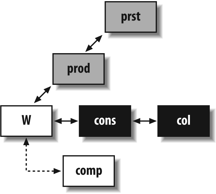
There are two interesting facts in this part of the query: first, prod and prst logically belong to a subquery, and because w is nothing but a glue table, it can go with them.
The second interesting fact is that comp is externally joined, but nothing is returned from it and there is no condition whatsoever (besides the join condition) on its columns. That means that not only does comp not belong to the core query (it doesn’t contribute to shaping the result set), but in fact it doesn’t belong to the query at all. Very often, this type of error comes from an enthusiastic application of the cut ‘n’ paste programming technique. The join with comp is totally useless in this part of the query. The only thing it might have contributed to is to multiply the number of rows returned, a fact artfully [38] hidden by the use of distinct, which is not necessary because union does away with duplicate rows, too.
The second part of the union, which I have represented in Figure 5-8, tells a different story. As in the first part of the union, prst, prod, and w can go to a subquery. In this case, though, comp is necessary because I can say that it links what is returned (data from cons and col) to the tables that allow us to define exactly which rows from cons and col we want. But there is something weird in the join: the outer join between comp and w tells the SQL engine “complete what you return from w with null values in lieu of the columns from comp if you cannot find a match in comp.” So far, so good, except that comp is also linked—and with a regular, inner join—to cons on the other side. It is a sound practice to challenge any construct that doesn’t fall in the “plain and basic” category, and outer joins are neither plain nor basic. Let’s suppose that for one row provided by w we don’t find a match in comp. Then a null value is returned for comp.cons_id, which is used for the join with cons. A null value is never equal to anything else, and no row from cons will ever match it. Rows that will be returned in this part of the query can correspond only to cases when there is a match between w and comp. The conclusion is immediate: the join between w and comp should be an inner join, not an outer one. The outer join adds no value, but as it is a potentially more tolerant join than the regular inner join, it may well send a wrong signal to the optimizer and contribute to poor performance.
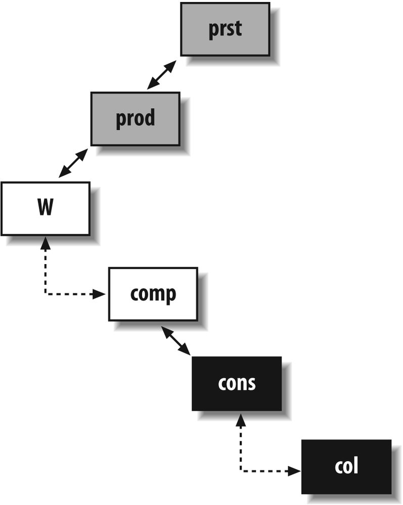
Now, prst, prod, w, and comp can all be moved to a subquery, as in the first part of the union. I can rewrite the query as follows:
select cons.id,
       coalesce(cons.definite_code, cons.provisional_code) dc,
       cons.name,
       cons.supplier_code,
       cons.registration_date,
       col.rco_name
from constituent cons
     left outer join cons_color col
             on col.rcolor_id = cons.rcolor_id
where cons.id in (select w.id
                  from weighing w
                       inner join production prod
                               on prod.id = w.id
                       inner join process_status prst
                               on prst.prst_id = prod.prst_id
                  where prod.usr_id = :userid
                   and prst.prst_code = 'PENDING')
union
select  cons.id,
       coalesce(cons.definite_code, cons.provisional) dc,
       cons.name,
       cons.supplier_code,
       cons.registration_date,
       cons.flash_point,
       col.rco_name
from constituent cons
     left outer join cons_color col
             on col.rcolor_id = cons.rcolor_id
where cons.id in (select comp.cons_id
                  from composition comp
                       inner join weighing w
                               on w.formula_id = comp.formula_id
                             inner join production prod
                                     on prod.id = w.id
                             inner join process_status prst
                                     on prst.prst_id = prod.prst_id
                  where prod.usr_id = :userid
                 and prst.prst_code = 'PENDING')
If I now consider the subquery as a whole, instead of having the union of two mighty joins, I can relegate the union to a subquery in a kind of factorization:
select cons.id,
       coalesce(cons.definite_code, cons.provisional_code) dc,
       cons.name,
       cons.supplier_code,
       cons.registration_date,
       col.rco_name
from constituent cons
     left outer join cons_color col
             on col.rcolor_id = cons.rcolor_id
where cons.id in (select w.id
                  from weighing w
                       inner join production prod
                               on prod.id = w.id
                       inner join process_status prst
                               on prst.prst_id = prod.prst_id
                  where prod.usr_id = :userid
                   and prst.prst_code = 'PENDING
                  union
                  select comp.cons_id
                  from composition comp
                       inner join weighing w
                               on w.formula_id = comp.formula_id
                             inner join production prod
                                     on prod.id = w.id
                             inner join process_status prst
                                     on prst.prst_id = prod.prst_id
                  where prod.usr_id = :userid
                 and prst.prst_code = 'PENDING')
In the real case from which I derived this example, I had excellent performance at this point (runtime had dropped from more than a minute to about 0.4 seconds) and I stopped here. I still have a repeating pattern, though: the repeated pattern is the join between w, prod, and prst. In the first part of the new union, the id column from w is returned, whereas in the second part, the formula_id column from the same table is used to join to comp.
If performance had still been unsatisfactory, I might have tried, with Oracle or SQL Server, to use the with clause to factorize the repeated query:
with q as (select w.id, w.formula_id
           from weighing w
           inner join production prod
                   on prod.id = w.id
           inner join process_status prst
                   on prst.prst_id = prod.prst_id
           where prod.usr_id = :userid
             and prst.prst_code = 'PENDING')
In that case, the union would have become:
select q.id
from q
union
select comp.cond_id
from composition comp
         inner join q
                 on q.formula_id = comp.formula_id
I’d like to point out that at this stage all of the modifications I applied to the query were of a purely logical nature: I gave no consideration to the size of tables, their structures, or the indexes on them. Sometimes a logical analysis is enough. Often, though, once the logical structure of the query has been properly identified and you have a clean, straight frame, it is time to look more closely at the data to reconstruct the query. The problem with SQL is that many constructs are logically equivalent (or almost logically equivalent, as you will see). Choosing the right one may be critical, and all DBMS products don’t necessarily handle all constructs identically. Nowhere is this as flagrant as with subqueries.
Playing with Subqueries
You can use subqueries in many places, and it is important to fully understand the implications of all alternative writings to use them correctly and to avoid bugs. In this section, I will review the most important places where you can use subqueries and discuss potential implications.
Subqueries in the select list
The first place you can have subqueries is the select list; for instance, something such as the following:
select a.c1, a.c2, (select some_col from b where b.id = a.c3) as sub
from a ...
Such a subquery has a constraint: it cannot return more than one row (this type of subquery is sometimes called a scalar subquery). However, it can return no row at all, in which case the sub column will appear as a null value in the result. As a general rule, subqueries in the select list are correlated to the outer query: they refer to the current row of the main query, through the equality with a.c3 in the previous example.
If the optimizer doesn’t try to rewrite the whole query or to cache intermediate results, the subquery will be fired for every row that is returned. This means that it can be a good solution for a query that returns a few hundred rows or less, but that it can become lethal on a query that returns millions of rows.
Even when the number of rows returned by the query isn’t gigantic, finding several subqueries hitting the same table is an unpleasant pattern. For instance (case 1):
select a.c1, a.c2,
       (select some_col from b where b.id = a.c3) as sub1,
       (select some_other_col from b where b.id = a.c3) as sub2,
       ...
from a ...
In such a case, the two queries can often be replaced by a single outer join:
select a.c1, a.c2,
       b.some_col as sub1,
       b.some_other_col as sub2,
       ...
from a
     left outer join b
                  on b.id = c.c3
The join has to be an outer join to get null values when no row from b matches the current row from a.
In some rare cases, though, adding a new outer join to the from clause is forbidden, because a single table would be outer-joined to two other different tables; in such a case, all other considerations vanish and the only way out is to use similar subqueries in the select list.
Case 1 was easy, because both subqueries address the same row from b. Case 2 that follows is a little more interesting:
select a.c1, a.c2,
       (select some_col
        from b
        where b.id = a.c3
          and b.attr = 'ATTR1') as sub1,
       (select some_other_col
        from b
        where b.id = a.c3
          and b.attr = 'ATTR2') as sub2,
       ...
from a ...
In contrast to case 1, in case 2 the subqueries are hitting two different rows from table b; but these two rows must be joined to the same row from table a. We could naturally move both subqueries to the from clause, aliasing b to b1 and b2, and have two external joins. But there is something more interesting to do: merging the subqueries.
To transform the two subqueries into one, you must, as in the simple case with identical where conditions, return some_col and some_other_col simultaneously. But there is the additional twist that, because conditions are different, we will need an or or an in and we will get not one but two rows. If we want to get back to a single-row result, as in case 1, we must squash the two rows into one by using the technique of a case combined with an aggregate, which you saw earlier in this chapter:
select id,
       max(case attr
             when 'ATTR1' then some_col
             else null
           end) some_col,
       max(case attr
             when 'ATTR2' then some_other_col
             else null
           end) some_other_col
from b
where attr in ('ATTR1', 'ATTR2')
group by id
By reinjecting this query as a subquery, but in the from clause this time, you get a query that is equivalent to the original one:
select a.c1, a.c2,
       b2.some_col,
       b2.some_other_col,
       ...
from a
     left outer join (select id,
                             max(case attr
                                   when 'ATTR1' then some_col
                                   else null
                                 end) some_col,
                             max(case attr
                                   when 'ATTR2' then some_other_col
                                   else null
                                 end) some_other_col
                      from b
                      where attr in ('ATTR1', 'ATTR2')
                      group by id) b2
                   on b2.id = a.c3
As with case 1, the outer join is necessary to handle the absence of any matching value. If in the original query one of the values can be null but not both values at the same time, a regular inner join would do.
Which writing is likely to be closer to the most efficient execution of the query? It depends on volumes, and on existing indexes.
The first step when tuning the original query with the two scalar subqueries will probably be to ensure that table b is properly indexed. In such a case, an index on (id, attr) is what I would expect. But when I replace the two scalar subqueries with an aggregate, the join between a.c3 and b.id is suddenly relegated to a later stage: I expect the aggregate to take place first, and then the join to occur. If I consider the aggregate alone, an index on (id, attr) will be of little or no help, although an index on (attr, id) might be more useful, because it would make the computation of the aggregate more efficient.
The question at this point is one of relative cardinality of id versus attr. If there are many values for attr relative to id, an index in which attr appears in the first position makes sense. Otherwise, we have to consider the performance of a full scan of b combined with an aggregate executed only once, versus the performance of a fast indexed query executed (on this example) twice by row that is returned. If table b is very big and the number of rows returned by the global query is very small, scalar subqueries may be faster; in all other cases, the query that uses scalar subqueries will probably be outperformed by the query that uses the from clause subquery.
Subqueries in the from clause
Contrary to subqueries in the select list, subqueries in the from clause are never correlated. They can execute independently from the rest. Subqueries in the from clause serve two purposes:
Performing an operation that requires a sort, such as a
distinctor agroup byon a lesser volume than everything that is returned by the outer query (which is what I did in the previous example)Sending the signal “this is a fairly independent piece of work” to the optimizer
Subqueries in the from clause are very well defined as inline views in the Oracle literature: they behave, and are often executed, as views whose lifespan is no longer than the execution of the query.
Subqueries in the where clause
Contrary to subqueries in the select list or in the from clause, subqueries in the where clause can be either correlated to the outer query or uncorrelated. In the first case, they reference the “current row” of the outer query (a typical example of a correlated subquery is and exists ()). In the second case, the subqueries can execute independently from the outer query (a typical example is and column_name in () [39]). From a logical point of view, they are exchangeable; if, for instance, you want to identify all the registered users from a website who have contributed to a forum recently, you can write something like this:
select m.member_name, ...
from members m
where exists (select null
              from forum f
              where f.post_date >= ...
                and f.posted_by = m.member_id)
or like this:
select m.member_name, ...
from members m
where m.member_id in (select f.posted_by
                      from forum f
                      where f.post_date >= ...)
But there are two main differences between the two preceding code snippets:
A correlated subquery must be fired each time the value from the outer query changes, whereas the uncorrelated subquery needs to be fired only once.
Possibly more important is the fact that when the query is correlated, the outer query drives execution. When the query is uncorrelated, it can drive the outer query (depending on other criteria).
Because of these differences, an uncorrelated subquery can be moved almost as is to the from clause. Almost, because in () performs an implicit distinct, which must become explicit in the from clause. Thus, we also can write the preceding example as follows:
select m.member_name ...
from members m
     inner join (select distinct f.posted_by
                 from forum f
                 where f.post_date >= ...) q
              on q.posted_by = m.member_id
As you may remember from Chapter 1, various DBMS products exhibit a different affinity to alternative writings. As a result, we can kick a table out of the from clause during the first stage of our analysis because it implements only an existence test, and we can bring it back to the from clause if the DBMS likes joining inline views better than in ().
But you must fully understand the differences between the two writings. In the previous query, the distinct applies to the list of member identifiers found in the forum table, not to all the data that is returned from members. We have, first and foremost, a subquery.
The choice between correlated and uncorrelated subqueries isn’t very difficult to make, and some optimizers will do it for you; however, the fact is often forgotten that assumptions about indexing are different when you use a correlated and an uncorrelated subquery, because it’s no longer the same part of the query that pulls the rest. An optimizer will try its best with available indexes, and will not create indexes (although a “tuning wizard,” such as the tuning assistants available with some products, might suggest them).
It all boils down to volume. If your query returns few rows, and the subquery is used as an additional and somewhat ancillary condition, a correlated subquery is a good choice. It may be a good choice too if the equivalent in () subquery would return hundreds of thousands of rows, because writing something such as the following would make little sense:
and my_primary_key in (subquery that returns plenty of rows)
If you really want to access many rows, you don’t want to use an index, even a unique index. In such a case, you have two possibilities:
The expected result set is really big, and the best way to obtain the result set is through methods such as hash joins (more about joins later); in such a case, I’d move the subquery to the
fromclause.The expected result set is small, and you are courting disaster. Suppose that for some reason the optimizer fails to get a proper estimate about the number of rows returned by the subquery, and expects this number of rows to be small. It will be very tempted to ignore the other conditions (some of which must be very selective) and focus on the reference to the primary key, and it will have everything wrong. In such a case, you are much better off with a correlated subquery.
I came across a very interesting case while writing this book. The query that was causing worry was from a software package, and there was no immediate way to modify the code. However, by monitoring SQL statements that were executed, I traced the reason for slowness to a condition that involved an uncorrelated subquery:
...
and workset.worksetid in
                (select tasks.worksetid
                 from tasks
                 where tasks.projectversion = ?)
...
The tasks table was a solid, 200,000-row table. Indexing a column named projectversion was obviously the wrong idea, because the cardinality of the column was necessarily low, and the rest of the query made it clear that we were not interested in rare project version numbers. Although I didn’t expect to be able to modify the query, I rewrote it the way I would have written it originally, and replaced the preceding condition with the following:
and exists (select null
            from tasks
            where tasks.worksetid = workset.worksetid
              and tasks.projectversion = ?)
That was enough to make me realize something I had missed: there was no index on the worksetid column of the tasks table. Under the current indexing scheme, a correlated subquery would have been very slow, much worse than the uncorrelated subquery, because the SQL engine would have to scan the tasks table each time the value of worksetid in the outer query changed. The database administrator rushed to create an index on columns (worksetid, projectversion) of the tasks table on the test database and, without changing the text of the query, the running time suddenly fell from close to 30 seconds down to a few hundredths of a second. What happened is that the optimizer did the same transformation as I had; however, now that indexing had been adjusted to make the correlated subquery efficient, it was able to settle for this type of subquery, which happened to be the right way to execute the query. This proves that even when you are not allowed to modify a query, rewriting it may help you better understand why it is slow and find a solution.
Activating Filters Early
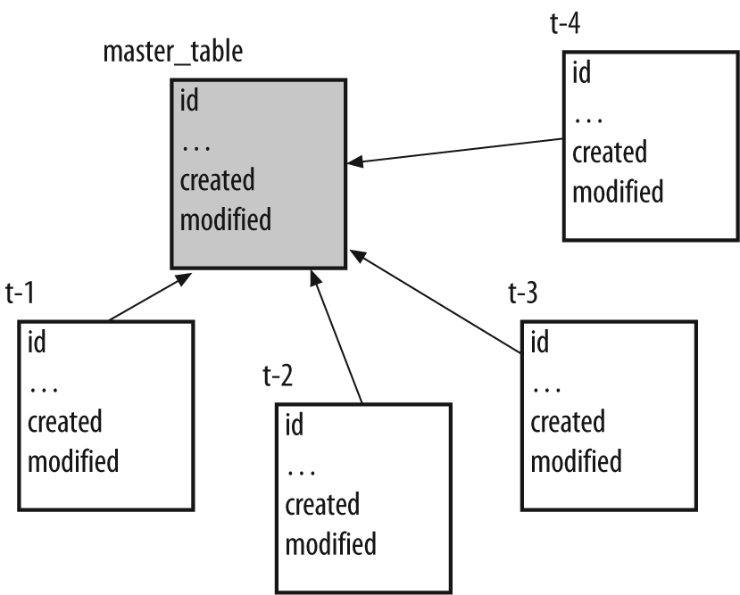
Another important principle, filtering, must be brought into the process as soon as possible. This means you should eliminate rows before joining, sorting, or aggregating, and not after. I already mentioned the classic where versus having case, in which it sometimes makes a tremendous difference (particularly if the optimizer doesn’t fix your mistakes behind your back) to eliminate rows before aggregation when conditions don’t bear on the result of aggregation. But there are other common cases. Take, for instance, a schema that looks like the one in Figure 5-9, where a master table contains some basic information about a number of items, and peripheral tables contain attributes for these items that may or may not be present. All tables contain the item’s identifier as well as two columns that specify when the row was created (mandatory column) or last modified (which can be null if the row was never modified since creation). The task was to provide a list of all items that had been modified as of a given date.
I once found this task performed by the following code: [40]
select ...
from master_table m
     left outer join t1
                  on t1.id = master_table.id
     left outer join t2
                  on t2.id = master_table.id
     left outer join t3
                  on t3.id = master_table.id
     left outer join t4
                  on t4.id = master_table.id
where (case
         when coalesce(m.modified, m.created) > some_date then 1
         when coalesce(t1.modified, t1.created) > some_date then 1
         when coalesce(t2.modified, t2.created) > some_date then 1
         when coalesce(t3.modified, t3.created) > some_date then 1
         when coalesce(t4.modified, t4.created) > some_date then 1
         else 0
       end) = 1
The tables involved were not huge; all of them stored between thousands and tens of thousands of rows. But the query was very slow and ultimately returned few rows. The small result set meant that few records were modified during the period under scrutiny, and that the condition on the date was very selective. But to be able to deal with all the created and modified dates within a single expression, the SQL engine must first perform all joins—which is a lot of work on five tables of this size when no efficient filtering condition is applied before the join.
The answer in such a case is to identify the core query as the (small) set of identifiers that relate to rows recently modified. As such, we can rewrite the core query as follows:
select id from master_table where coalesce(m.modified, m.created) >some_dateunion select id from t1 where coalesce(t1.modified, t1.created) >some_dateunion select id from t2 where coalesce(t2.modified, t2.created) >some_dateunion select id from t3 where coalesce(t3.modified, t3.created) >some_dateunion select id from t4 where coalesce(t4.modified, t4.created) >some_date
Even when each select translates to a table scan, we end up scanning a volume that comprises hundreds of thousands of rows—in other words, not very much compared to filtering after the join. The implicit distinct and the resultant sort called for by union will operate on a small number of identifiers, and you quickly get a very short list of identifiers. As a result, you have managed to perform screening before the joins, and you can proceed from here to retrieve and join the few rows of interest, which will be an almost instantaneous process.
Simplifying Conditions
Once you have checked that no function is applied to a column that prevents using an efficient index on that column, there isn’t much you can do to improve regular equality or inequality conditions. But we aren’t done with subqueries. Even when we have chosen whether a subquery should be correlated or uncorrelated, we may realize that we have many conditions that are now expressed as subqueries (possibly as a result of our cleaning up the from clause).
Therefore, the next step is to minimize the number of subqueries. One of your guiding principles must be to visit each table as few times as possible (if you have studied operational research, think of the traveling salesman problem [41]). You can encounter a number of patterns where hitting each table only once is easy:
If several subqueries refer to the same table, check whether all the information cannot be collected in a single pass. This type of rewriting is usually easier with uncorrelated subqueries. So, when you have something such as this:
and c1 in (select col1 from
t1where ...) and c2 in (select col2 fromt1where ...)where
c1andc2don’t necessarily refer to columns from the same table in the outer query, it is sometimes possible, depending on the “compatibility” of the twowhereclauses, to have a single query that returns bothcol1andcol2. Then, you can move the subquery up in thefromclause as an inline view (not forgetting to adddistinctif necessary), and join with it.Conversely, when the same column from the outer query is related to various subqueries that hit different tables, as shown here:
and
c1in (select col1 from t1 where ...) andc1in (select col2 from t2 where ...)it may be interesting to combine the two subqueries with the
intersectset operator if available, or with a simple join:and c1 in (select col1 from t1 inner join t2 on t2.col1 = t1.col1 where ...)Another relatively common pattern is subqueries that implement a sort on two keys—namely, “I want the text associated to an identifier for the most recent date for which I have text for this identifier, and within that date I want the highest version number if I find several matching rows.” You will often find such a condition coded as follows:
select t.text
from t
where t.textdate = (select max(x.textdate)
                     from t as x
                     where  x.id = t.id)
  and t.versionnumber = (select max(y.versionnumber)
                         from t as y
                         where y.id = t.id
                           and y.textdate = t.textdate)
order by t.id
Two such subqueries can actually be merged with the outer query. With Oracle or SQL Server, I would use a ranking function:
select x.text
from (select id,
             text,
             rank() over (partition by id
                          order by textdate desc,
                                   versionnumber desc) as rnk
      from t) x
where x.rnk = 1
order by x.id
With MySQL, I would sort by
idand, as in the previous case, by descendingtextdateandversionnumber. To display only the most recent version of the text for eachid, I would make tricky use of a local variable named@idto “remember” the previousidvalue and show only those rows for whichidisn’t equal to the previous value. Because of the descending sort keys, it will necessarily be the most recent one.The really tricky part is the fact that I must at once compare the current
idvalue to@idand assign this current value to the variable for the next row. I do this by usinggreatest(), which needs to evaluate all of its arguments before returning, and evaluates them from left to right. The first argument ofgreatest()—the logical functionif(), which compares the column value to the variable—returns0if they are equal (in which case the DBMS mustn’t return the row) and1if they are different. The second argument ofgreatest()is a call toleast()to which I pass first0, which will be returned and will have no impact on the result ofgreatest(), plus an expression that assigns the current value ofidto@id. When the call toleast()has been evaluated, the correct value has been assigned to the variable and I am ready to process the next row. As a finishing touch, a dummyselectinitializes the variable. Here is what it gives when I paste all the components together:select x.text from (select a.text, greatest(if(@id = id, 0, 1), least(0, @id := id)) must_show from t a, (select @id := null) b order by a.id, a.textdate desc, a.versionnumber desc) x where x.must_show = 1Naturally, this is a case where you can legitimately question the assertion that SQL allows you to state what you want without stating how to obtain it, and where you can wonder whether the word simplifying in the title of this section isn’t far-fetched. Nevertheless, there are cases when this single query allows substantial speed gains over a query that multiplies subqueries.
Other Optimizations
Many other optimizations are often possible. Don’t misunderstand my clumping them together as their being minor improvements to try if you have time; there are cases where they can really save a poorly performing query. But they are variations on other ideas and principles exposed elsewhere in this chapter.
Simplifying aggregates
As you saw earlier, aggregates that are computed on the same table in different subqueries can often be transformed in a single-pass operation. You need to run a query on the union of the result sets returned by the various subqueries and carefully use the case construct to compute the various sums, counts, or whatever applied to each subset.
Using with
Both Oracle and SQL Server know of with, which allows you to assign a name to a query that may be run only once if it is referred to several times in the main query. It is common, in a big union statement, to find exactly the same subquery in different select statements in the union. If you assign a name to this subquery at the beginning of the statement, as shown here:
with my_subquery as (select distinct blah from ...)
you can replace this:
where somecol in (select blah from ...)
with this:
where somecol = my_subquery.blah
The SQL engine may decide (it will not necessarily do it) to execute my_subquery separately, keep its result set in some temporary storage, and reuse that result set wherever it is referenced.
Because it can work with only uncorrelated subqueries, using with may mean turning some correlated subqueries into uncorrelated subqueries first.
Combining set operators
The statements that most often repeat SQL patterns are usually statements that use set operators such as union. Whenever you encounter something that resembles the following:
select ...
from a, b, t1
where ...
union
select ...
from a, b, t2
where ...
you should wonder whether you couldn’t visit tables a and b, which appear in both parts of the statement, fewer times. You can contemplate a construct such as this one:
select ...
from a, b,
     (select ...
      from t1
      where ...
      union
      select ...
      from t2
      where ...)
where ...
The previous rewrite may not always be possible—for instance, if table b is joined on one column to t1 in the first part of the statement, and on a different column to t2 in the second part. But you mustn’t forget that there may be other intermediate possibilities, such as this:
select ...
from a,
     (select ...
      from b, t1
      where ...
      union
      select
      from b, t2
      where ...)
where ...
Without carefully studying the various criteria that comprise a query, table indexing, and the size of the intermediate result sets, there is no way you can predict which alternative rewrite will give the best results. Sometimes the query that repeats patterns and visits the various tables several times delivers superior performance, because there is a kind of reinforcement of the various criteria on the different tables that makes each select in the statement very selective and very fast. But if you find these repeated patterns while investigating the cause of a slow query, don’t forget to contemplate other combinations.
Rebuilding the Initial Query
Once the query core has been improved, all you have to do is to bring back into the query all the tables that, because they didn’t contribute to the identification of the result set, had been scraped off in our first stage. In technical terms, this means joins.
There are basically two methods for an SQL engine to perform joins. [42] Joins are essentially a matching operation on the value of a common column (or several columns in some cases). Consider the following example:
select a.c2, b.col2 from a, b where a.c3 =<some value>and a.c1 = b.col1 and b.col3 =<some other value>
Nested Loops
The method that probably comes most naturally to mind is the nested loop: scanning the first table (or the result set defined by restrictive conditions on this table), and then for each row getting the value of the join column, looking into the second table for rows that match this value, and optionally checking that these rows satisfy some other conditions. In the previous example, the SQL engine might:
Scan table
afor rows that satisfy the condition onc3.Check the value of
c1.Search the
col1column in thebtable for rows that match this value.Verify that
col3satisfies the other condition before returning the columns in theselectlist.
Note that the SQL optimizer has a number of options, which depend on indexing and what it knows of the selectivity of the various conditions: if b.col1 isn’t indexed but a.c1 is, it will be much more efficient to start from table b rather than table a because it has to scan the first table anyway. The respective “quality” of the conditions on c3 and col3 may also favor one table over the other, and the optimizer may also, for instance, choose to screen on c3 or col3 before or after the matching operation on c1 and col1.
Merge/Hash Joins
But there is another method, which consists of processing, or preparing, the two tables involved in the join before matching them.
Suppose that you have coins to store into a cash drawer, where each type of coin goes into one particular area of the insert tray. You can get each coin in turn, look for its correct position, and put it in its proper place. This is a fine method if you have few coins, and it’s very close to the nesting loop because you check coins one by one as you would scan rows one by one. But if you have many coins to process, you can also sort your coins first, prepare stacks by face value, and insert all your coins at once. This is sort of how a merge join works. However, if you lack a workspace where you can spread your coins to sort them easily, you may settle for something intermediate: sorting coins by color rather than face value, then doing the final sort when you put the coins into the tray. This is vaguely how a hash join works.
With the previous example, joining using this method would mean for the SQL engine:
Dealing with, say, table
afirst, running filtering on columnc3Then either sorting on column
c1, or building a hash table that associates to a computation on the value ofc1pointers to the rows that gave that particular resultThen (or in parallel) processing table
b, filtering it oncol3Then sorting the resultant set of rows on
col1or computing hash values on this columnAnd finally, matching the two columns by either merging the two sorted result sets or using the hash table
Sometimes nested loops outperform hash joins; sometimes hash joins outperform nested loops. It depends on the circumstances. There is a very strong affinity between the nested loop and the correlated subquery, and between the hash or merge join and the uncorrelated subquery. If you execute a correlated subquery as it is written, you do nothing but a nested loop. Nested loops and correlated subqueries shine when volumes are low and indexes are selective. Hash joins and uncorrelated subqueries stand out when volumes are very big and indexes are either inefficient or nonexistent.
You must realize that whenever you use inline views in the from clause, for instance, you are sending a very strong “hash join” signal to the optimizer. Unless the optimizer rewrites the query, whenever the SQL engine executes an inline view, it ends up with an intermediate result set that it has to store somewhere, in memory or in temporary storage. If this intermediate result set is small, and if it has to be joined to well-indexed tables, a nested loop is an option. If the intermediate result is large or if it has to be joined to another intermediate result for which there can be no index, a merge or hash join is the only possible route. You can therefore (re)write your queries without using heavy-handed “directives,” and yet express rather strongly your views on how the optimizer should run the query (while leaving it free to disagree).
[37] It happens more often than it should, particularly when a query has been derived from another existing query rather than written from scratch.
[38] As in “Oops, I have duplicate rows—oh, it’s much better with distinct….”
[39] I once encountered a correlated in() statement, but unsurprisingly, it drove the optimizer bananas.
[40] The actual query was using the greatest() function that exists in both MySQL and Oracle, but not in SQL Server. I have rewritten the query in a more portable way.
[41] Given a number of cities and the distances between them, what is the shortest round-trip route that visits each city exactly once before returning to the starting city?
[42] I am voluntarily ignoring some specific storage tricks that allow us to store as one physical entity two logically different tables; these implementations have so many drawbacks in general usage that they are suitable for only very specific cases.