Computation-only functions are (usually) pretty harmless, although it can be argued that when you code with SQL, it’s not primarily in functions that you should incorporate computations, unless they are very specific:^[20] computed columns in views are the proper place to centralize simple to moderately complex operations. Whenever you call a function, a context switch slows down execution, but unless your function is badly written (and this isn’t specific to databases), you cannot hope for much performance gain by rewriting it. The only case when rewriting can make a significant difference is when you can make better use of primitive built-in functions. Most cases I have seen of poor usage of built-in functions were custom string or date functions, especially when some loop was involved.

I will give you an example of a user-written function in Oracle that is much more efficient when it makes extensive use of built-in functions: the counting of string patterns. Counting repeating patterns is an operation that can be useful in a number of cases, and you’ll find an application of this operation at the end of this chapter. Let’s state the problem in these terms: we are given a string haystack and a pattern needle, and we want to return how many times needle occurs in haystack.

One way to write this function is the way I wrote it in function1:

create or replace function function1(p_needle   in varchar2,
                                     p_haystack in varchar2)
return number
is
  i   number := 1;
  cnt number := 0;
begin
  while (i <= length(p_haystack))
  loop
    if (substr(p_haystack, i, length(p_needle)) = p_needle)
    then
      cnt := cnt + 1;
    end if;
    i := i + 1;
  end loop;
  return cnt;
end;
/

This is standard code that uses two built-in functions, length() and substr(). We can improve it a little, if we don’t want to count overlapping patterns, by increasing the index by the length of needle instead of by 1 each time we find a match.

However, we can write it a different way (function2) by using the Oracle-specific function instr(), which returns the position of a substring within a string. instr() takes two additional parameters: the start position within the string and the occurrence (first, second, etc.) of the substring we search. function2 takes advantage of the occurrence parameter, increasing it until nothing is found:

create or replace function function2(p_needle   in varchar2,
                                     p_haystack in varchar2)
return number
is
  pos        number;
  occurrence number := 1;
begin
  loop
    pos := instr(p_haystack, p_needle, 1, occurrence);
    exit when pos = 0;
    occurrence := occurrence + 1;
  end loop;
  return occurrence - 1;
end;
/

I removed the loop in function3 by comparing the length of the initial searched string haystack to the length of the string after replacing all occurrences of needle with an empty string; I just need to divide the difference by the length of needle to determine how many times the pattern occurs. Contrary to the previous functions, I no longer use any Oracle-specific implementation. (You may remember that I used this method in the preceding chapter to count separators in a string that contained a list of values I wanted to bind.)

create or replace function function3(p_needle   in varchar2,
                                     p_haystack  in varchar2)
return number
is
begin
  return (length(p_haystack)
          - length(replace(p_haystack, p_needle, '')))
           /length(p_needle);
end;
/

To compare functions, I created a table and populated it with 50,000 strings of random lowercase letters, with a random length of between 5 and 500:

create table test_table(id number,
                        text varchar2(500))
/
begin
  dbms_random.seed(1234);
  for i in 1 .. 50000
  loop
     insert into test_table
     values(i, dbms_random.string('L', dbms_random.value(5, 500)));
  end loop;
  commit;
end;
/

Finally, I compared all three functions by counting in my test tables how many strings contain more than 10 occurrences of the letters s, q, and l, respectively:

select count(*)
from test_table
where functioni('s', text) > 10
/
select count(*)
from test_table
where functioni('q', text) > 10
/
select count(*)
from test_table
where functioni('l', text) > 10
/

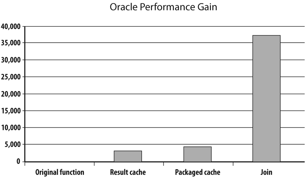
I ran this test with each of the three functions, summed up elapsed times (all three nearly identical), and divided 150,000 (the total number of rows I scanned) by the total elapsed time to compare the number of rows scanned per second in all three cases. You can see the result of the experiment in Figure 3-1.

Figure 3-1. Three different ways to implement pattern counting with Oracle

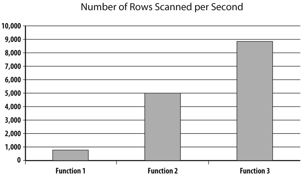
The original function that loops on strings is about 10 times less efficient than the function that makes creative use of replace(), with the loop on instr() halfway between the two others. It would probably not be a waste of your time to carefully read the documentation regarding the built-in functions provided with your DBMS; reinventing the wheel, even if your code avoids gross inefficiencies, doesn’t pay. But suffice it to say that as the respective throughputs show, improving a function of moderate complexity can bring ample rewards in a batch program.

The Oracle and SQL Server optimizers know one particular kind of function: deterministic functions. A function is deterministic if it always returns the same value when you call it with the same parameters. SQL Server decides by itself whether a function is deterministic. Oracle relies on your stating that it is by adding the deterministic keyword after the declaration of the type of value returned by the function (MySQL 5.1 knows the keyword but the optimizer ignores it). If a function is deterministic, the DBMS “remembers” a number of associations between the parameters and the returned value, and returns the result without actually calling the function whenever it is invoked with the same parameters. This caching of function results can bring impressive performance gains, but it is beneficial only when we call the function with relatively few different parameters. The previous example of a function looking for patterns would not benefit from being declared deterministic (even if it is), because one of the parameters, the text string to scan, is different each time. However, in many cases the same parameters are used again and again. This is particularly true when we apply functions to dates, because very often processes are applied to a relatively narrow range of dates, with the same date occurring many times.

You must be very careful about determinism; sometimes a function isn’t deterministic for a reason that comes from an unexpected corner. A typical example is the function that returns the number representing a day in the week, something you obtain by applying to your date column to_char(date_column, 'D') with Oracle, datepart(dw, date_column) with SQL Server, or dayofweek(date_column) with MySQL. Except in the case of MySQL, where the function returns the ISO day-of-week number, the function is not deterministic because it depends on internationalization settings and local conventions. And as you can see in the following Oracle example, conventions may be different even in countries that are geographically very close:

SQL> alter session set nls_territory=spain;

Session altered.

SQL> select to_char(to_date('1970/01/01', 'YYYY/MM/DD'), 'D')
  2  from dual;

TO_CHAR(TO_DATE('1970/01/01','YYYY/MM/DD'),'D')
---------------------------------------------------------------------------
4

SQL> alter session set nls_territory=portugal;

Session altered.

SQL> select to_char(to_date('1970/01/01', 'YYYY/MM/DD'), 'D')
  2  from dual;

TO_CHAR(TO_DATE('1970/01/01','YYYY/MM/DD'),'D')
---------------------------------------------------------------------------
5

SQL> alter session set nls_territory=morocco;

Session altered.

SQL> select to_char(to_date('1970/01/01', 'YYYY/MM/DD'), 'D')
  2  from dual;

TO_CHAR(TO_DATE('1970/01/01','YYYY/MM/DD'),'D')
---------------------------------------------------------------------------
6

Oracle has a workaround with a conversion to the name of the day, which optionally takes a parameter that specifies the language in which the name must be returned:

ORACLE-SQL> alter session set nls_language=american;

Session altered.

SQL> select to_char(to_date('1970/01/01', 'YYYY/MM/DD'),
  2                 'DAY', 'NLS_DATE_LANGUAGE=ITALIAN')
  3  from dual;

TO_CHAR(TO_DATE('1970/01/01','YYYY/MM/DD'),'DAY','NLS_DATE_LANGUAGE=ITALIAN
---------------------------------------------------------------------------
GIOVEDI

SQL> select to_char(to_date('1970/01/01', 'YYYY/MM/DD'), 'DAY')
  2  from dual;

TO_CHAR(TO_DATE('1970/01/01','YYYY/MM/DD'),'DAY')
---------------------------------------------------------------------------
THURSDAY

SQL> alter session set nls_language=german;

Session altered.

SQL> select to_char(to_date('1970/01/01', 'YYYY/MM/DD'),
  2                 'DAY', 'NLS_DATE_LANGUAGE=ITALIAN')
  3  from dual;

TO_CHAR(TO_DATE('1970/01/01','YYYY/MM/DD'),'DAY','NLS_DATE_LANGUAGE=ITALIAN
---------------------------------------------------------------------------
GIOVEDI

SQL> select to_char(to_date('1970/01/01', 'YYYY/MM/DD'), 'DAY')
  2  from dual;

TO_CHAR(TO_DATE('1970/01/01','YYYY/MM/DD'),'DAY')
---------------------------------------------------------------------------
DONNERSTAG

The regular manner with SQL Server to cast in bronze what will be returned by datepart(dw, …) is to call set datefirst, which cannot be done in a function. There is a way out, though: comparing what the function returns with what the same function applied to a known date returns. From the results kindly provided by Oracle, we know that January 1, 1970 was a Thursday; if the function returns the same thing we get with January 3, 1970, we have a Saturday, and so on.

Keeping in mind how to return with Oracle a truly deterministic identification of days, I can now write a function that returns 1 if a date corresponds to a weekend day (i.e., Saturday or Sunday) and 0 otherwise. To see the benefits of using Oracle to declare a function as deterministic, I will create two identical functions, one that isn’t declared deterministic and one that is:

SQL> create or replace function weekend_day(p_date in date)
  2  return number
  3  is
  4    wday   char(3);
  5  begin
  6    wday := substr(to_char(p_date, 'DAY',
  7                   'NLS_DATE_LANGUAGE=AMERICAN'), 1, 3);
  8    if (wday = 'SAT') or (wday = 'SUN')
  9    then
 10       return 1;
 11    else
 12       return 0;
 13    end if;
 14  end;
 15  /

Function created.

Elapsed: 00:00:00.04
SQL> create or replace function weekend_day_2(p_date in date)
  2  return number
  3  deterministic
  4  is
  5    wday   char(3);
  6  begin
  7    wday := substr(to_char(p_date, 'DAY',
  8                   'NLS_DATE_LANGUAGE=AMERICAN'), 1, 3);
  9    if (wday = 'SAT') or (wday = 'SUN')
 10    then
 11       return 1;
 12    else
 13       return 0;
 14    end if;
 15  end;
 16  /

Function created.

Elapsed: 00:00:00.02

Now, suppose we have a table that records sales, associating to each sale a date and an amount, and say that we want to compare the total amount sold during weekends with the total amount sold during the rest of the week for the past month. Let’s run the query twice, with the nondeterministic function first and the deterministic function afterward:

SQL> select sum(case weekend_day(sale_date)
  2            when 1 then 0
  3            else sale_amount
  4          end) week_sales,
  5          sum(case weekend_day(sale_date)
  6            when 0 then 0
  7            else sale_amount
  8          end) week_end_sales
  9  from sales
 10  where sale_date >= add_months(trunc(sysdate), -1)
 11  /

WEEK_SALES WEEK_END_SALES
---------- --------------
 191815253     73131546.8

Elapsed: 00:00:11.27
SQL> select sum(case weekend_day_2(sale_date)
  2            when 1 then 0
  3            else sale_amount
  4          end) week_sales,
  5          sum(case weekend_day_2(sale_date)
  6            when 0 then 0
  7            else sale_amount
  8          end) week_end_sales
  9  from sales
 10  where sale_date >= add_months(trunc(sysdate), -1)
 11  /

WEEK_SALES WEEK_END_SALES
---------- --------------
 191815253     73131546.8

Elapsed: 00:00:11.24

The results are not that convincing. Why? Actually, my query violates one of the conditions I specified for the efficiency of deterministic functions: being called with the same parameters again and again. The Oracle date type is equivalent to the datetime type of other DBMS products: it contains a time element, to a precision of one second. Needless to say, I was careful when generating my test data to generate values of sale_date at various times of the day. Let’s suppress the time element by applying the trunc() function to the data, which sets time to 00:00:00, and let’s try again:

SQL> select sum(case weekend_day(trunc(sale_date))
  2            when 1 then 0
  3            else sale_amount
  4          end) week_sales,
  5          sum(case weekend_day(trunc(sale_date))
  6            when 0 then 0
  7            else sale_amount
  8          end) week_end_sales
  9  from sales
 10  where sale_date >= add_months(trunc(sysdate), -1)
 11  /

WEEK_SALES WEEK_END_SALES
---------- --------------
 191815253     73131546.8

Elapsed: 00:00:12.69
SQL> select sum(case weekend_day_2(trunc(sale_date))
  2            when 1 then 0
  3            else sale_amount
  4          end) week_sales,
  5          sum(case weekend_day_2(trunc(sale_date))
  6            when 0 then 0
  7            else sale_amount
  8          end) week_end_sales
  9  from sales
 10  where sale_date >= add_months(trunc(sysdate), -1)
 11  /

WEEK_SALES WEEK_END_SALES
---------- --------------
 191815253     73131546.8
Elapsed: 00:00:02.58

Under suitable circumstances, the deterministic function allows the query to run five times faster.

You must be aware that declaring with Oracle that a function is deterministic isn’t something to be taken lightly.

To explain, imagine that we have a table of employees, and that employees may be assigned to projects through a table called project_assignment that links an employee number to a project identifier. We could issue a query such as the following to find out which projects are currently assigned to people whose last name is “Sharp”:

SQL> select e.lastname, e.firstname, p.project_name, e.empno
  2  from employees e,
  3       project_assignment pa,
  4       projects p
  5  where e.lastname = 'SHARP'
  6    and e.empno = pa.empno
  7    and pa.project_id = p.project_id
  8    and pa.from_date < sysdate
  9    and (pa.to_date >= sysdate or pa.to_date is null)
 10  /

LASTNAME             FIRSTNAME            PROJECT_NAME      EMPNO
-------------------- -------------------- ----------------- ----------
SHARP                REBECCA              SISYPHUS                2501
SHARP                REBECCA              DANAIDS                 2501
SHARP                MELISSA              DANAIDS                 7643
SHARP                ERIC                 SKUNK                   7797

A similar type of query returns the only “Crawley” and the project to which he is assigned:

SQL> select e.lastname, e.firstname, p.project_name
  2  from employees e,
  3        project_assignment pa,
  4        projects p
  5  where e.lastname = 'CRAWLEY'
  6    and e.empno = pa.empno
  7    and pa.project_id = p.project_id
  8    and pa.from_date < sysdate
  9    and (pa.to_date >= sysdate or pa.to_date is null)
 10  /

LASTNAME             FIRSTNAME            PROJECT_NAME        
-------------------- -------------------- --------------------
CRAWLEY              RAWDON               SISYPHUS            

Now let’s suppose that for some obscure reason someone has written a lookup function that returns the name associated with an employee number capitalized in a more glamorous way than the full uppercase used in the tables:

SQL> create or replace function NameByEmpno(p_empno in number)
  2  return varchar2
  3  is
  4      v_lastname varchar2(30);
  5  begin
  6      select initcap(lastname)
  7      into v_lastname
  8      from employees
  9      where empno = p_empno;
 10      return v_lastname;
 11  exception
 12      when no_data_found then
 13           return '*** UNKNOWN ***';
 14  end;
 15  /

Someone else now decides to use this function to return the employee/project association without explicitly joining the employees table:

SQL> select p.project_name, pa.empno
  2  from projects p,
  3       project_assignment pa
  4  where pa.project_id = p.project_id
  5    and namebyempno(pa.empno) = 'Sharp'
  6    and pa.from_date < sysdate
  7    and (pa.to_date >= sysdate or pa.to_date is null)
  8  /

PROJECT_NAME              EMPNO
-------------------- ----------
SKUNK                      7797
SISYPHUS                   2501
DANAIDS                    7643
DANAIDS                    2501

Analysis reveals that indexing the function would make the query faster:

SQL> create index my_own_index on project_assignment(namebyempno(empno))
  2  /
create index my_own_index on project_assignment(namebyempno(empno))
                                                *
ERROR at line 1:
ORA-30553: The function is not deterministic

Undaunted, our developer modifies the function, adds the magical deterministic keyword, and successfully creates the index.

I would really have loved to elaborate on the romantic affair that developed around the coffee machine, but I’m afraid that O’Reilly is not the proper publisher for that kind of story. Suffice it to say that one day, Mr. Crawley proposed to Miss Sharp and his proposal was accepted. A few months later, the marriage led to a data change at the hands of someone in the HR department, following a request from the new Mrs. Crawley:

SQL> update employees set lastname = 'CRAWLEY' where empno = 2501;

1 row updated.

SQL> commit;

Commit complete.

What happens to the project queries now? The three-table join no longer sees any Rebecca Sharp, but a Rebecca Crawley, as can be expected:

SQL> select e.lastname, e.firstname, p.project_name
  2  from employees e,
  3       project_assignment pa,
  4       projects p
  5  where e.lastname = 'SHARP'
  6    and e.empno = pa.empno
  7    and pa.project_id = p.project_id
  8    and pa.from_date < sysdate
  9    and (pa.to_date >= sysdate or pa.to_date is null)
 10  /

LASTNAME             FIRSTNAME            PROJECT_NAME
-------------------- -------------------- --------------------
SHARP                MELISSA              DANAIDS
SHARP                ERIC                 SKUNK

SQL> select e.lastname, e.firstname, p.project_name
  2  from employees e,
  3       project_assignment pa,
  4       projects p
  5  where e.lastname = 'CRAWLEY'
  6    and e.empno = pa.empno
  7    and pa.project_id = p.project_id
  8    and pa.from_date < sysdate
  9    and (pa.to_date >= sysdate or pa.to_date is null)
 10  /

LASTNAME             FIRSTNAME            PROJECT_NAME
-------------------- -------------------- --------------------
CRAWLEY              REBECCA              SISYPHUS
CRAWLEY              RAWDON               SISYPHUS
CRAWLEY              REBECCA              DANAIDS

For the query that uses the function, and the function-based index, nothing has changed:

SQL> select p.project_name, pa.empno
  2  from projects p,
  3        project_assignment pa
  4  where pa.project_id = p.project_id
  5    and namebyempno(pa.empno) = 'Crawley'
  6    and pa.from_date < sysdate
  7    and (pa.to_date >= sysdate or pa.to_date is null)
  8  /

PROJECT_NAME              EMPNO
-------------------- ----------
SISYPHUS                   2503

SQL> select p.project_name, pa.empno
  2  from projects p,
  3        project_assignment pa
  4  where pa.project_id = p.project_id
  5    and namebyempno(pa.empno) = 'Sharp'
  6    and pa.from_date < sysdate
  7    and (pa.to_date >= sysdate or pa.to_date is null)
  8  /

PROJECT_NAME              EMPNO
-------------------- ----------
SKUNK                      7797
SISYPHUS                   2501
DANAIDS                    7643
DANAIDS                    2501

The reason is simple: indexes store key values and addresses; they duplicate some information, and DBMS products routinely return data from indexes when the only information needed from the table is contained in the index. The table has been updated, but not the index. Our present key is stored in the index. We have said that the function is deterministic and that it always returns the same value for the same set of parameters. That means the result should never change. Therefore, the DBMS believes this assertion, doesn’t attempt to rebuild or invalidate the index when the base table is changed (which would be totally impractical anyway), and returns wrong results.

Obviously, the previous function could not be deterministic because it was a lookup function, querying the database. Fortunately, we sometimes have other means to improve lookup functions, and we will explore them now.

Lookup functions can provide fertile ground for spectacular improvement. By embedding database access inside a precompiled function, the original developer wanted to turn the function into a building block. Rather than a building block, you should have another image in mind: a black box, because that’s what the function will look like to the optimizer. Whenever you call a lookup function inside a query, the queries that run inside the function are insulated from what happens outside, even if they are hitting the same tables as the calling statement; in particular, there are strong odds that if you aren’t careful, queries that are hidden inside a function will be executed every time the function is called.

Estimating how many times a function may be called is the key to estimating how much it contributes to poor performance. This is true of any function, but more so of lookup functions, because even a fast database access is comparatively much costlier than the computation of a mathematical or string expression. And here you must once again distinguish between two cases, namely:

If we consider the very worst case, a lookup function that happens to be the only criterion inside the where clause, we end up with what is, in effect, a straightjacketed nested loop: a table will be scanned, and for each row the function will be called and will access another table. Even if the SQL query in the function is very fast, you will kill performance. I called the loop straightjacketed because the optimizer will be given no chance to choose a different plan, such as joining the two tables (the one to which the function is applied and the one that is queried in the function) through merging or hashing. Worse, in many cases the lookup function will always be called with the same parameters to always return the same values, not truly deterministic, but “locally deterministic,” within the scope of the user session or batch run.

Now I will use two different examples of lookup functions, and I will show you how you can improve them in some cases, even when they look rather plain.

Example 1: A calendar function

The first function is called NextBusinessDay(), takes a date as a single parameter, and returns a date that is computed in the following manner:

• If the parameter is a Friday, we add three days to it (we are in a country where neither Saturday nor Sunday is a business day).

• If the parameter is a Saturday, we add two days.

• Otherwise, we add one day.

• We then check the result against a table that contains all the dates of public holidays for the range of dates of interest. If we find a public holiday that matches the date we have found, we iterate. Otherwise, we are done.

Being aware of the number-of-the-day-in-the-week issue, here is how I can code the function, first with Oracle:

create or replace function NextBusinessDay(this_day in date)
return date
as
  done     boolean := false;
  dow      char(3);
  dummy    number;
  nextdate date;
begin
  nextdate := this_day;
  while not done
  loop
     dow := substr(to_char(nextdate, 'DAY',
                   'NLS_DATE_LANGUAGE=AMERICAN'), 1, 3);
     if (dow = 'FRI')
     then nextdate := nextdate + 3;
     elsif (dow = 'SAT')
          then nextdate := nextdate + 2;
     else nextdate := nextdate + 1;
     end if; 
     begin
       select 1
       into dummy
       from public_holidays
       where day_off = nextdate;
     exception
       when no_data_found then
           done := true;
     end;
  end loop; 
  return nextdate;
end;
/

Then with SQL Server:

create function NextBusinessDay(@this_day date)
returns date
as
begin
  declare @done     bit;
  declare @dow      char(1);
  declare @dummy    int;
  declare @nextdate date;
  set @nextdate = @this_day;
  set @done = 0;
  while @done = 0
  begin
     set @dow = datepart(dw, @nextdate);
     if @dow = datepart(dw, convert(date, '01/02/1970', 101))
       set @nextdate = @nextdate + 3;
     else
       if @dow = datepart(dw, convert(date, '01/03/1970', 101))
         set @nextdate = @nextdate + 2;
       else
         set @nextdate = @nextdate + 1;
     set @dummy = (select 1
                   from public_holidays
                   where day_off = @nextdate);
     if coalesce(@dummy, 0) = 0
     begin
       set @done = 1;
     end;
  end; 
  return @nextdate;
end;

And finally with MySQL (for which I don’t need to worry about what dayofweek() returns):

delimiter //
create function NextBusinessDay(this_day datetime)
returns date
reads sql data
begin
  declare done     boolean default 0;
  declare dow      smallint;
  declare dummy    smallint;
  declare nextdate date;
  declare continue handler for not found set done = 1;
  set nextdate = date(this_day);
  while not done do
     set dow = dayofweek(nextdate);
     case dow
       when 6 then set nextdate = date_add(nextdate, interval 3 day);
       when 7 then set nextdate = date_add(nextdate, interval 2 day);
       else        set nextdate = date_add(nextdate, interval 1 day);
     end case; 
     select 1
     into dummy
     from public_holidays
     where day_off = nextdate;
  end while; 
  return nextdate;
end;
//
delimiter ;

I use the same one-million-row table containing sales dates as I did when I added up the sales that took place on weekend days and sales from other weekdays. Then I simply run a select NextBusinessDay(sale_date)… over all the rows of my table.

For reasons that will soon be obvious, I mostly used Oracle for my tests.

On my machine, the simple test took about two and a half minutes to return all one million rows—a throughput of 6,400 rows per second. Not dismal, but the statistics kindly provided by Oracle^[21] report two million recursive calls; these calls comprise the function call and the query inside the function. It’s a mighty number when you consider that we have only 121 different days in the table. Because rows were presumably entered chronologically,^[22] in most cases the result of the function applied to a row will be exactly the same as the result for the previous row.

How can I improve performance without touching the code that calls the function? One possibility, if the DBMS supports it, is to ask the SQL engine to cache the result of the function. Caching the function result is not as stringent as defining the function as deterministic: it just says that as long as the tables on which the function relies are not modified, the function can cache results and can return them again when it is called with the same parameters. Such a function will not allow us, for instance, to create an index on its result, but it will not reexecute when it is not needed.

Oracle introduced the caching of function results in Oracle 11g; MySQL 5.1 doesn’t cache the result of queries that are called in a function, and SQL Server 2008 doesn’t allow caching that is any more explicit than specifying that a function returns null when input is null (which can speed up evaluation in some cases). With Oracle, I have therefore re-created my function, simply modifying its heading in the following way:

create or replace function NextBusinessDay(this_day in date)
return date
result_cache relies_on(public_holidays)
as ...

The optional relies_on clause simply tells Oracle that the cached result may need to be flushed if the public_holidays table is modified.

Running the same test as before yielded a very bad result: my throughput went down by 30% or so, to 4,400 rows per second. The reason is exactly the same as we already saw in the case of the deterministic function: because the dates also store a time part that varies, the function is almost never called with the same parameter. We get no benefit from the cache, and we pay the overhead due to its management.

If I don’t want to modify the original code, I can cheat. I can rename my previous cached function as Cached_NextBusinessDay() and rewrite the function that is called in the statement as follows:

create or replace function NextBusinessDay(this_day in date)
return date
as
begin
  return(Cached_NextBusinessDay(trunc(this_day)));
end;

Running the same query, my table scan took a little more than 30 seconds, or a throughput of 31,700 rows per second, almost five times my initial throughput. This ratio is in the same neighborhood as the ratio obtained by stating that a function was deterministic, without all the constraints linked to having a truly deterministic function. If you want to improve lookup functions, caching their result is the way to go.

But what if my DBMS doesn’t support caching function results? We still have some tricks we can apply by taking advantage of the fact that rows are, more or less, stored in chronological order. For instance, every version of Oracle since Oracle 7 (released in the early 1990s) supports using variables in a package to cache the previous results. Packaged variables aren’t shared among sessions. You first define your function inside a package:

create or replace package calendar
is
    function NextBusinessDay(this_day in date)
    return date;
end;
/

Then you create the package body, in which two variables, duly initialized, store both the last input parameter and the last result. You must be careful that the lifespan of the cache is the duration of the session; in some cases, you may have to build an aging mechanism. In the function, I check the current input parameter against the past one and return the previous result without any qualms if they are identical; otherwise, I run the query that is the costly part of the function:

create or replace package body calendar
is

    g_lastdate   date := to_date('01/01/0001', 'DD/MM/YYYY'),
    g_lastresult date := NULL;

    function NextBusinessDay(this_day in date)
    return date
    is
       done     boolean := false;
       dow      char(3);
       dummy    number;
     begin
       if (this_day <> g_lastdate)
       then
         g_lastdate := this_day;
         g_lastresult := this_day;
         while not done
         loop
            dow := substr(to_char(g_lastresult, 'DAY',
                          'NLS_DATE_LANGUAGE=AMERICAN'), 1, 3);
            if (dow = 'FRI')
            then g_lastresult := g_lastresult + 3;
            elsif (dow = 'SAT')
                 then g_lastresult := g_lastresult + 2;
            else g_lastresult := g_lastresult + 1;
            end if; 
            begin
              select 1
              into dummy
              from public_holidays
              where day_off = g_lastresult;
            exception
              when no_data_found then
                  done := true;
            end;
         end loop; 
       end if;
       return g_lastresult;
     end;

end;

Finally, to keep the interface identical, I rewrite the initial function as a mere wrapper function that calls the function in the package, after removing the time part from the date:

create or replace function NextBusinessDay(this_day in date)
return date
as
begin
  return calendar.NextBusinessDay(trunc(this_day));
end;

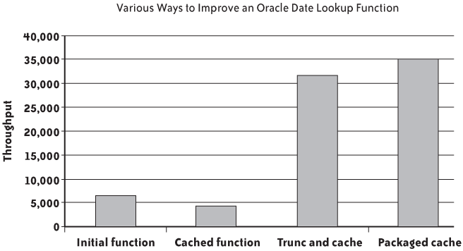
The good news for people who are running older Oracle versions is that in this case (i.e., when I process dates in more or less chronological order), I get an even better result than when I let Oracle manage the cache: my test run was almost 10% faster, achieving a throughput of 34,868 rows per second. However, keep in mind that the Oracle cache is not dependent on the order of the dates, but simply on there having been a limited number of dates. Figure 3-2 summarizes the variations of throughput by rewriting my NextBusinessDay() function in different ways.

It is interesting to note that the result_cache clause can either noticeably degrade or boost performance depending on whether it has been used in the wrong or right circumstances.

Can we apply any of the improvement methods that work with Oracle to other products? It depends. Explicitly asking for the function result to be cached is, at the time of this writing, something specific to Oracle, as are packages. Unfortunately, SQL Server offers no way to manually cache the result of functions written in T-SQL, because it only knows of local variables that exist only for the duration of the function call, and because temporary tables, which are the closest you can come to global variables, cannot be referenced in a function.

Figure 3-2. How the throughput of the same Oracle lookup function varies

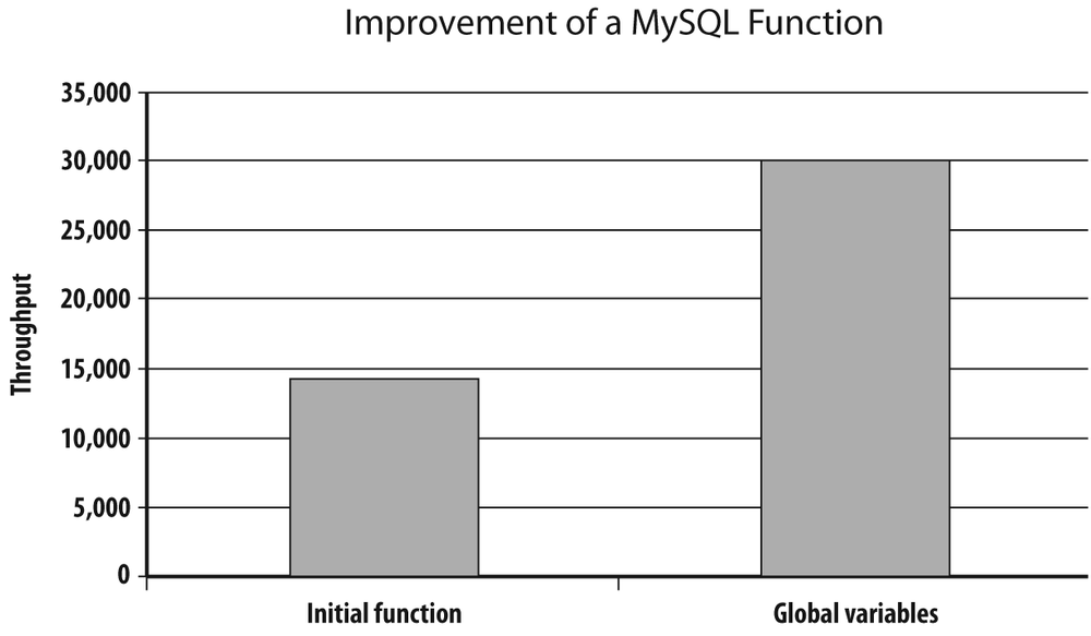
Although MySQL 5.1 can cache the result of queries, it cannot cache the result of queries run from inside a function or procedure. However, contrary to T-SQL, MySQL allows referencing global session variables inside a function, and session variables can be used for buffering results. The only snag is that, whereas Oracle’s packaged variables are private when defined in the package body and invisible outside the package, the MySQL session variables are accessible to any function. Giving them very common names (e.g., @var1) is therefore courting disaster, and if you want to stay on the safe side you should use long, unwieldy names that minimize the risk of accidental collision. In the following example, I systematically use <function name>$ as a prefix:

delimiter //
create function NextBusinessDay(this_day datetime)
returns date
reads sql data
begin
 declare done     boolean default 0;
 declare dow      smallint;
 declare dummy    smallint;
 declare continue handler for not found set done = 1;
 if (ifnull(@NextBusinessDay$last_date, '1769-08-15') <> date(this_day))
 then
  set @NextBusinessDay$last_date = date(this_day);
  set @NextBusinessDay$last_business_day = date(this_day);
  while not done do
   set dow = dayofweek(@NextBusinessDay$last_business_day);
   case dow
    when 6 then
       set @NextBusinessDay$last_business_day =  
            date_add(@NextBusinessDay$last_business_day, interval 3 day);
    when 7 then
       set @NextBusinessDay$last_business_day =
            date_add(@NextBusinessDay$last_business_day, interval 2 day);
    else set @NextBusinessDay$last_business_day =
            date_add(@NextBusinessDay$last_business_day, interval 1 day);
   end case; 
   select 1
   into dummy
   from public_holidays
   where day_off = @NextBusinessDay$last_business_day;
  end while; 
 end if;
 return @NextBusinessDay$last_business_day;
end;
//
delimiter ;

As you can see in Figure 3-3, implementing in MySQL the same ideas as with Oracle also brings a significant performance improvement when scanning chronologically ordered rows.

Figure 3-3. Using variables to cache the result of a MySQL function

Example 2: A conversion function

The second function, called FxConvert(),^[23] takes two parameters—an amount and a currency code—and returns the amount converted into a predefined reference currency at the most recent available conversion rate. Here I am using the tables used in the Chapter 1 example. You can use FxConvert() as a prototype for transcoding functions.

Here is the original code for Oracle:

create or replace function FxConvert(p_amount   in number,
                                     p_currency in varchar2)
return number
is
  n_converted    number;
begin
  select p_amount * a.rate
  into n_converted
  from currency_rates a
  where (a.iso, a.rate_date) in
      (select iso, max(rate_date) last_date
       from currency_rates
       where iso = p_currency
       group by iso);
  return n_converted;
exception
  when no_data_found then
      return null;
end;
/

Here is the code for SQL Server:

create function fx_convert(@amount   float,
                           @currency char(3))
returns float
as
begin
  declare @rate  float;
  set @rate = (select a.rate
               from currency_rates a
                    inner join (select iso,
                                       max(rate_date) last_date
                                from currency_rates
                                where iso = @currency
                                group by iso) b
                            on a.iso = b.iso
                           and a.rate_date = b.last_date);
  return coalesce(@rate, 0) * @amount;
end;

And here is the code for MySQL:

delimiter //
create function FxConvert(p_amount float, p_currency char(3))
returns float
reads sql data
begin
  declare converted_amount float;
  declare continue handler for not found set converted_amount = 0;
  select a.rate * p_amount
  into converted_amount
  from currency_rates a
       inner join (select iso, max(rate_date) last_date
                   from currency_rates
                   where iso = p_currency
                   group by iso) b
               on a.iso = b.iso
              and a.rate_date = b.last_date;
  return converted_amount;
end;
//
delimiter ;

Let’s start, as we did before, with Oracle. We have basically two ways to improve the function: either use the result_cache keyword for Oracle 11g and later, or use packaged variables and “manually” handle caching.

If I want result_cache to be beneficial, I need to modify the function so as to have a limited number of input parameters; because there may be a large number of different amounts, the amount value must be taken out of the equation. I therefore redefine the function as a wrapper of the real function for which results will be cached:

create or replace function FxRate(p_currency in varchar2)
return number
result_cache relies_on(currency_rates)
is
  n_rate    number;
begin
  select rate
  into n_rate
  from (select rate
        from currency_rates
        where iso = p_currency
        order by rate_date desc)
  where rownum = 1;
  return n_rate;
exception
  when no_data_found then
      return null;
end;
/
create or replace function FxConvert(p_amount   in number,
                                     p_currency in varchar2)
return number
is
begin
  return p_amount * FxRate(p_currency);
end;
/

If I want to handle caching through packaged variables, I cannot use two variables as I did in the NextBusinessDay() example. I was implicitly relying on the fact that the function was successively evaluated for the same date. In this example, even if I have a limited number of currencies, the currency codes will be alternated instead of having long runs of identical codes that would benefit from “remembering” the previous value.

Instead of simple variables, I use a PL/SQL associative array, indexed by the currency code:

create or replace package fx
as

  function rate(p_currency in varchar2)
  return number;

end;
/

create or replace package body fx
as
  type t_rates is table of number
                  index by varchar2(3);
  a_rates  t_rates;
  n_rate   number;

  function rate(p_currency in varchar2)
  return number
  is
    n_rate number;
  begin
    begin
      n_rate := a_rates(p_currency);
    exception
      when no_data_found then
        begin
          select a.rate
          into a_rates(p_currency)
          from currency_rates a
          where (a.iso, a.rate_date) in
              (select iso, max(rate_date) last_date
               from currency_rates
               where iso = p_currency
               group by iso);
          n_rate := a_rates(p_currency);
        end;
    end;
    return n_rate;
  end;

end;
/
create or replace function FxConvert(p_amount   in number,
                                     p_currency in varchar2)
return number
is
begin
  return p_amount * fx.rate(p_currency);
end;
/

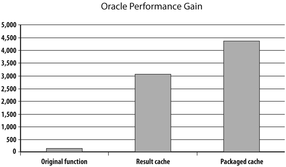
I tested the alternative versions of the function by running the following query against my two-million-row transactions table, using as a reference for 100 the number of rows scanned per second by the original function:

select sum(FxConvert(amount, curr))
from transactions;

Figure 3-4 shows the result.

At this point, I should put these performance gains into perspective. If you cannot touch the code, the rewrites I just presented can indeed result in an impressive improvement: the simple split of the function to use a result cache improved speed by a factor of 30 on my machine, and the more elaborate use of an array cache inside a package improved speed by a factor of 45. But remember that the function is a black box, and if you really want an impressive improvement with Oracle, there is no such thing as rewriting the test query as follows:

Figure 3-4. Comparison of alternative ways to write a currency-conversion function with Oracle

select sum(t.amount * r.rate )
from transactions t
     inner join
          (select a.iso, a.rate
           from (select iso,
                        max(rate_date) last_date
                 from currency_rates
                 group by iso) b
                inner join currency_rates a
                   on a.iso = b.iso
                  and a.rate_date = b.last_date) r
on r.iso = t.curr;

You’ll probably find this query more difficult to read than the one that uses the function, but in fact, the subquery that follows the first inner join is nothing more than the subquery in the function. I am using an inner join because the function ignores currencies for which the rate is unknown, and therefore, we need not bother about the few lines referring to very exotic currencies. Figure 3-5, which is Figure 3-4 with the replacement of the function call by the join, probably doesn’t need any comment.

What about the other products?

We have seen that unfortunately, options are very limited with T-SQL functions. I already mentioned that T-SQL doesn’t know of session variables. You could cheat and use managed code (a .NET language routine called by the SQL engine) to do the trick; for instance, you could use static variables in C#. Take such an idea out of your mind, however; in their great wisdom, Microsoft developers have decided that “assemblies” (i.e., interfaces between T-SQL and .NET language code) have, by default, a PERMISSION_SET value of SAFE.

Figure 3-5. An Oracle comparison of various rewrites of a function to a simple join

Therefore, if you try to use static variables in a managed code function, you’ll get the following error message:

CREATE ASSEMBLY failed because type '...' in safe assembly '...' has
a static field '...'. Attributes of static fields in safe assemblies
must be marked readonly in Visual C#, ReadOnly in Visual Basic, or
initonly in Visual C++ and intermediate language.

If you don’t want to play it safe, you can have static variables. But the problem is that in a DLL, they are shared by all sessions. When queries run concurrently, anything can happen.

To demonstrate this (and for once I will not give the code), I tested a C# function that converts currencies using two static variables and “remembers” the exchange rate and last currency encountered (in this case, this method is inefficient, but efficiency wasn’t my goal). I summed the converted amounts in my two-million-row transactions table.

If you run the query when you are the only connected session, you get, more slowly, the same result as the T-SQL function; that is:

782780436669.151

Now, running the same query using the C#-with-static-variables function against the same data in three concurrent sessions yielded the following results:

782815864624.758
782797493847.697
782816529963.717

What happened? Each session simply overwrote the static variables in turn, messing up the results—a good example of uncoordinated concurrent access to the same memory area.

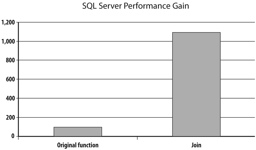
If refactoring a function, and one function alone, is not an option with SQL Server, replacing a lookup function with a join is often possible. The comparison of the query that calls the function with the query that uses the join, though not as impressive as with Oracle, is nevertheless impressive enough to give good hopes of improving speed when a function that can be merged inside the query is used. The result of my tests is shown in Figure 3-6.

Figure 3-6. An SQL Server performance comparison of repeatedly calling a simple lookup function versus a join

As we have seen, with MySQL you can use session variables. However, in the case of currencies, and noting the need to remember several exchange rates, we must be a little creative because MySQL knows no array variable. Instead of using an array, I concatenate the currency codes into one string and the matching exchange rates into another; built-in functions allow me to identify the position of one code in the string and to isolate the matching exchange rate, converting the string into a float value by adding 0.0 to it. To stay on the safe side, I define a maximum length for my strings:

delimiter //
create function FxConvert(p_amount float, p_currency char(3))
returns float
reads sql data
begin
  declare pos      smallint;
  declare rate     float;
  declare continue handler for not found set rate = 0;
  set pos = ifnull(find_in_set(p_currency,
                               @FxConvert$currency_list), 0);
  if pos = 0
  then
    select a.rate
    into rate
    from currency_rates a
         inner join (select iso, max(rate_date) last_date
                     from currency_rates
                     where iso = p_currency
                     group by iso) b
                 on a.iso = b.iso
                and a.rate_date = b.last_date;
    if (ifnull(length(@FxConvert$rate_list ), 0) < 2000
            and ifnull(length(@FxConvert$currency_list), 0) < 2000)
    then
      set @FxConvert$currency_list = concat_ws(',',
                                               @FxConvert$currency_list,
                                               p_currency);
      set @FxConvert$rate_list = concat_ws('|',
                                           @FxConvert$rate_list,
                                           rate);
    end if;
  else
    set rate = 0.0 + substring_index(substring_index(@FxConvert$rate_list,
                               '|', pos), '|', -1);
  end if;
  return p_amount * rate;
end;
//
delimiter ;

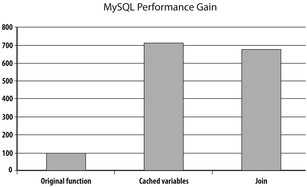
I won’t pretend that the resultant code is elegant or that hand-crafted associative arrays are very easy to maintain. But the performance gain is here, and interestingly, the rewritten function performs even slightly better than the join, as you can see in Figure 3-7.

Figure 3-7. Substantially rewriting the conversion function with MySQL

As the preceding currency conversion example shows, it is sometimes much more efficient to rewrite a statement to get rid of the function entirely. Instead of executing a call, you can reinject the database accesses you find in the function as joins or subqueries, which may be easy if the function is simple, or more difficult if the function includes procedural logic. (I will discuss how you can graft procedural logic into a statement in more detail in Chapter 6.) There are two major advantages to getting rid of functions:

The disadvantages are as follows:

Your choices are also sometimes limited by political reasons: if you are asked to refactor application A, and you find out that you could tremendously improve performance by reworking function F, which queries tables from a different functional domain, you may not have direct access to these tables. And if function F is also a cornerstone, in another functional domain, of applications B and C, for which no performance issue has so far been reported, touching F can trigger vicious turf wars if personal rivalries step in. In that case, adding a layer as a special wrapper function called FA that calls the original function F is often the best solution if you can limit in FA the number of calls to F.

I stated at the beginning of this chapter that views are the SQL equivalent of functions; in many cases—and the currency conversion is a good example—creating a view over the join that replaces the function would have provided a simple and efficient interface. But even views can sometimes have a negative impact on performance, as you will see next.

Views can serve several purposes. At their simplest (and most innocent), they can serve as a security device, narrowing the vision of data to some columns, or to some rows, or to some combination of rows and columns. Because all DBMS products feature information functions that retrieve data specific to the current user (such as the login name or system username), a generic view can be built that returns data dependent on the privileges of the invoker. Such a view merely adds filtering conditions to a base table and has no measurable impact on performance.

But views can also be repositories for complicated SQL operations that may have to be reused. And here it becomes much more interesting, because if we don’t keep in mind the fact that we are operating against a view and not a base table, in some cases we may suffer a severe performance penalty.

In this section, I will show how even a moderately complex view can impact performance through two examples drawn on two of the tables I used in Chapter 1: the transactions table, which contains amounts for many transactions carried out in different currencies, and the currency_rates table, which stores the exchange rate for the various currencies at various dates.

First let’s create a “complex” view that is no more than an aggregate of transactions by currency (in the real world, there likely would be an additional condition on dates, but the absence of this condition changes nothing in this example):

create view v_amount_by_currency
as select curr, round(sum(amount), 0) amount
   from transactions
   group by curr;

I haven’t picked a view that aggregates values at random; the problem with aggregating and filtering lies in whether you first aggregate a large volume of data and then filter on the result, or whether you filter first so as to aggregate a much smaller amount of data. Sometimes you have no choice (when you want to filter on the result of the aggregation, which is the operation performed by the having clause), but when you have the choice, what you do first can make a big difference in performance.

The question is what happens when you run a query such as the following:

select *
from v_amount_by_currency
where curr = 'JPY'; 

You have two options. You can apply filtering after the aggregate, like so:

select curr, round(sum(amount), 0) amount
from transactions
group by curr
having curr = 'JPY';

Or you can push the filtering inside the view, which behaves as though the query were written as follows:

select curr, round(sum(amount), 0) amount
from transactions
where curr = 'JPY'
group by curr;

You can consider this last query to be the “optimal” query, which I will use as a reference.

What happens when we query through the view actually depends on the DBMS (and, of course, on the DBMS version). MySQL 5.1 runs the view statement and then applies the filter, as the explain command shows:

mysql> explain select * from v_amount_by_currency 
    -> where curr = 'JPY';
+----+-------------+--------------+-//--------+---------------------------------+
| id | select_type | table        | //        |                                 |
+----+-------------+--------------+-//--------+---------------------------------+
|  1 | PRIMARY     | <derived2>   | //    170 | Using where                     |
|  2 | DERIVED     | transactions | //2000421 | Using temporary; Using filesort |
+----+-------------+--------------+-//--------+---------------------------------+
2 rows in set (3.20 sec)

There is a MySQL extension to the create view statement, algorithm=merge, that you can use to induce MySQL to merge the view inside the statement, but group by makes it inoperative.

On the Oracle side, the execution plan shows that the optimizer is smart enough to combine the view and the filtering condition, and to filter the table as it scans it, before sorting the result and performing the aggregation:

---------------------------------------------------------------------------...
| Id  | Operation            | Name         | Rows  | Bytes | Cost (%CPU)| ...
---------------------------------------------------------------------------...
|   0 | SELECT STATEMENT     |              |     1 |    12 |  2528   (3)| ...
|   1 |  SORT GROUP BY NOSORT|              |     1 |    12 |  2528   (3)| ...
|*  2 |   TABLE ACCESS FULL  | TRANSACTIONS |   276K|  3237K|  2528   (3)| ...
---------------------------------------------------------------------------...

Predicate Information (identified by operation id):
---------------------------------------------------
   2 - filter("CURR"='JPY')

This is in marked contrast to how Oracle behaves when it encounters a having clause in a regular statement. The upbeat Oracle optimizer assumes that developers know what they are writing and that having is always to be applied after the aggregate. Like the Oracle optimizer, the SQL Server optimizer pushes the where condition applied to the view inside the view. However, being less confident in human nature than its Oracle counterpart, the SQL Server optimizer is also able to push a condition that can be applied before aggregation inside the where clause when it appears in a having clause.

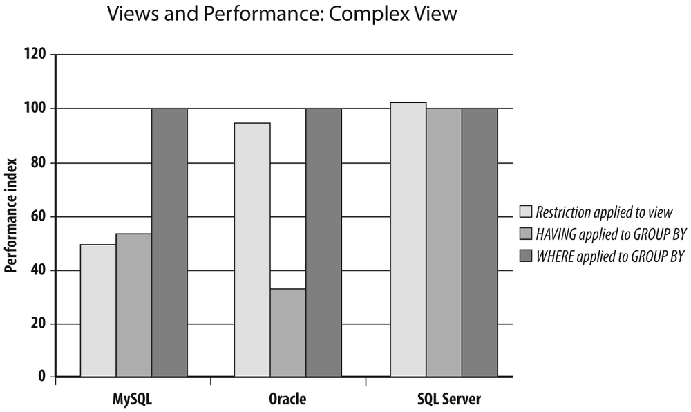
Figure 3-8 shows how the view performs comparatively to the “optimal” query that filters before aggregation and the query that uses having when it shouldn’t. There is a severe penalty with MySQL both when the view is used and when the having clause is misused; there is a stronger penalty with Oracle when filtering is wrongly performed through having, but there is hardly any impact when using the view. Performance is identical in all three cases with SQL Server.

Take note, though, that the MySQL penalty also comes from my having mischievously applied my condition to the column that controls the grouping: the currency column. I would have experienced no (or hardly any) penalty if my condition had been applied to the aggregated amount, because in that case the where applied to the view would have been strictly equivalent to a having clause.

Figure 3-8. How a query against a complex view can compare to a query against a table

All things considered, the complexity of the previous view was rather moderate. So, I have refined my analysis by creating a “more complex” view that refers to a secondary utility view. Let’s start with this utility view, which returns for each currency the most recent exchange rate:

create view v_last_rate
as
select a.iso, a.rate
from currency_rates a,
     (select iso, max(rate_date) last_date
      from currency_rates
      group by iso) b
where a.iso= b.iso
and a.rate_date = b.last_date;

I can now build the more complex view, which returns the converted amount per currency, but isolates the currencies that are most important to the bank’s business and groups together as OTHER all currencies that represent a small fraction of business:

create view v_amount_main_currencies
as
select case r.iso
         when 'EUR' then r.iso
         when 'USD' then r.iso
         when 'JPY' then r.iso
         when 'GBP' then r.iso
         when 'CHF' then r.iso
         when 'HKD' then r.iso
         when 'SEK' then r.iso
         else 'OTHER'
       end currency,
       round(sum(t.amount*r.rate), 0) amount
from transactions t,
     v_last_rate r
where r.iso = t.curr
group by case r.iso
           when 'EUR' then r.iso
           when 'USD' then r.iso
           when 'JPY' then r.iso
           when 'GBP' then r.iso
           when 'CHF' then r.iso
           when 'HKD' then r.iso
           when 'SEK' then r.iso
           else 'OTHER'
         end;

Now I run the same test as with the simpler aggregate, by comparing the performance of the following code snippet to the performance of two functionally equivalent queries that still use the utility view:

select currency, amount
from v_amount_main_currencies
where currency = 'JPY'; 

First I place the condition on the currency in the having clause:

select t.curr, round(sum(t.amount) * r.rate, 0) amount
from transactions t,
     v_last_rate r
where r.iso = t.curr
group by t.curr, r.rate
having t.curr = 'JPY';

Then I place the condition on the currency in the where clause:

select t.curr, round(sum(t.amount) * r.rate, 0) amount
from transactions t,
     v_last_rate r
where r.iso = t.curr
  and t.curr = 'JPY'
group by t.curr, r.rate;

You can see the result in Figure 3-9. As you might have expected, the MySQL engine goes on computing the aggregate in the view, and then performs the filtering (as it does with having). The resultant performance is rather dismal in comparison to the query that hits the table with the filtering condition where it should be.

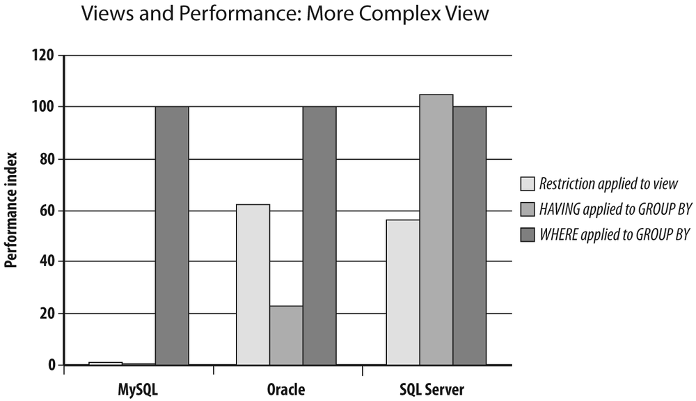
But the interesting and new fact in this rather hostile case is that even the Oracle and SQL Server optimizers cannot really keep query performance with the view on a par with the performance that can be obtained when correctly querying the table: the query against the view takes almost twice as long to run as the optimal query against the table.

The sample views I used are still simple views compared to some freak views I have come across; even a very smart optimizer will lose its footing when the view becomes quite complicated or when there are views stacked on one another.

Figure 3-9. Performance comparison with a more complex view

The optimizer isn’t necessarily to blame; sometimes it simply cannot decide what to do to improve performance.

Suppose, for instance, that we have a view defined as a join:

create view v(c1, c2, c3, c4, c5) as
select a.c1, a.c2, a.c3, b.c4, b.c5
from a, b
where a.c6 = b.c6

Now suppose that in a query all we require are columns c1 and c2, which both come from table a.

Do we need the join with table b? The answer may be either yes or no:

In other words, sometimes the join just provides additional columns, where this:

select c1, c2 from v

will return exactly the same rows as this:

select c1, c2 from a

And other times the query against the view will return fewer rows than the select from the table, because the join provides an additional filtering condition. In many cases, a human being will be able to decide what is or isn’t necessary to identify the proper result set, while the optimizer, very often because it lacks relevant information, will not be able to do so. In cases of doubt, the DBMS will always take the safest option: if you refer to the view, the optimizer will suppose, if it cannot decide otherwise, that the view may return a result set that is different from the result set returned by a simpler query, and it will use the view.

The more complex the view, the more ambiguities you may come across. Even a super-clever optimizer will be unable to decide how best to amalgamate the view to the query in all cases; moreover, a complex query means a very big number of options that it cannot explore in a limited amount of time. There is always a threshold where the optimizer gives up and the DBMS engine executes the view “as is” inside another query.

Earlier I mentioned joins that return columns that are unused in the query, which under certain conditions can translate into useless additional work. There are many other cases, especially when the query joins a view to a table that is already referenced inside a view. For instance, let’s suppose the query is built over an outer join:

select a.c1, a.c2, a.c3, b.c4, b.c5
from a
     left outer join b
          on b.c6 = a.c3

And let’s further suppose that this view is joined (with an inner join) inside a query to b, to return other information from b that doesn’t appear in the view. The inner join in the query is a stronger condition than the outer join in the view. In the context of the query, the outer join in the query might as well have been an inner join: rows for which there is no match between a and b will be returned by the view, but will be filtered out in the query. Every additional row returned because of the outer join is a waste in the context of the query—and an inner join might just have been much more efficient than an outer join.

You find very similar cases with views that are built as the union of several queries; you regularly find them used in queries that apply such filtering criteria that the result set can contain rows coming from only a small subset of the view, and we could have spared several possibly costly select statements.

A different, but no less perverse, effect of views on unsuspecting programmers is to induce them to base searches or joins on columns that are computed on the fly. Say, for instance, that one column in a table contains, for historical reasons, a Unix timestamp (the number of seconds elapsed since January 1, 1970, at 0:00 a.m.); this is the only table in the schema that doesn’t contain a regular SQL date, and therefore a developer decided to map over this table a simple view that masks the timestamp and converts it to a regular SQL date.

If an unsuspecting programmer innocently writes a condition such as the following:

where view_date_column = convert_to_date('date string')

this is what is really executed:

where convert_from_unix_timestamp(timestamp) = convert_to_date('date string')

Here we have a fine example of the dreaded case of the function applied to the indexed column, which prevents the use of the index. Unless an index has been computed—as Oracle and SQL Server may allow—on the converted timestamp,^[24] any date condition applied to the view is certain to not take advantage of an existing index on the raw timestamp.

Similarly, some developers are sometimes tempted to hide the ugliness of a very poor database design under views, and to make a schema look more normalized than it really is by splitting, for instance, a single column that contains multiple pieces of information. Such a Dorian Grayish attempt is pretty sure to backfire: filters and joins would be based not on real, indexed columns but on derived columns.

Many views are harmless, but if monitoring proves that some of the “problem queries” make use of complex views, these views should be one of your first targets. And because complex, underperforming views are often combinations of several views, you shouldn’t hesitate to rewrite views that are built on other views when they appear in problem queries; in many cases, you will be able to improve the performance of queries without touching them by simply redefining the views they reference. Views that are very complex should be made as simple as possible for the optimizer to work efficiently—not apparently simple, but simple in the sense that any trace of “fat” and unnecessary operations should be eliminated. If there is one place where the SQL code should be lean and mean, it is inside views. Rewriting views is, of course, the same skill as rewriting queries, which we will review in Chapter 5.

When you have doubts about views, querying the data dictionary can help you to spot complex views that you should rewrite. With MySQL, we can search the views’ text for the name of another view in the same schema, and for some keywords that indicate complexity. The following query counts for each view how many views it contains, as well as the number of subqueries—union, distinct or group by (here is the pattern counting in action):

select y.table_schema,
       y.table_name,
       y.view_len,
       y.referenced_views                                  views,
       cast((y.view_len - y.wo_from) / 4  - 1 as unsigned) subqueries,
       cast((y.view_len - y.wo_union) / 5 as unsigned)     unions,
       cast((y.view_len - y.wo_distinct) / 8 as unsigned)  distincts,
       cast((y.view_len - y.wo_group) / 5 as unsigned)     groups
from (select x.table_schema,
             x.table_name,
             x.view_len,
             cast(x.referenced_views as unsigned) referenced_views,
             length(replace(upper(x.view_definition), 'FROM', '')) wo_from,
             length(replace(upper(x.view_definition), 'UNION', '')) wo_union,
             length(replace(upper(x.view_definition), 'DISTINCT', '')) wo_distinct,
             length(replace(upper(x.view_definition), 'GROUP', '')) wo_group
      from (select v1.table_schema,
                   v1.table_name,
                   v1.view_definition,
                   length(v1.view_definition) view_len,
                   sum(case
                         when v2.table_name is not null
                          then (length(v1.view_definition)
                                 - length(replace(v1.view_definition,
                                                  v2.table_name, '')))
                                  /length(v2.table_name)
                         else 0
                       end) referenced_views
            from information_schema.views v1
                 left outer join information_schema.views v2
                              on v1.table_schema = v2.table_schema
            where v1.table_name <> v2.table_name
            group by v1.table_schema,
                     v1.table_name,
                     v1.view_definition) x
      group by x.table_schema,
               x.table_name) y
order by 1, 2;

The fact that Oracle stores the text of views in a long column prevents us from directly looking for keywords inside the view definition. We could do it with a little help from a PL/SQL stored procedure and conversion to a more amenable clob or a very large varchar2. However, we can get a very interesting indicator of view complexity thanks to the user_dependencies view that can be queried recursively when views depend on views:

col "REFERENCES" format A35
col name format A40
select d.padded_name name,
       v.text_length,
       d."REFERENCES"
from (select name,
             lpad(name, level + length(name)) padded_name,
             referenced_name || ' (' || lower(referenced_type) || ')' "REFERENCES"
      from user_dependencies
      where referenced_type <> 'VIEW'
      connect by prior referenced_type = type
          and prior referenced_name = name
      start with type = 'VIEW') d
     left outer join user_views v
          on v.view_name = name;

SQL Server allows both possibilities: querying information_schema.views or listing the hierarchy of dependencies available through sys.sql_dependencies. Although, to be frank, getting rid of duplicate rows and listing dependencies in a legible order requires a good deal of back-bending. The following query, which lists dependencies, is intended for a mature audience only:

with recursive_query(level,
                     schemaid,
                     name,
                     refschemaid,
                     refname,
                     reftype,
                     object_id,
                     ancestry) as
(select 1 as level,
        x.schema_id as schemaid,
        x.name,
        o.schema_id as refschemaid,
        o.name as refname,
        o.type_desc as reftype,
        o.object_id,
        cast(x.rn_parent + '.'
             + cast(dense_rank() over (partition by x.rn_parent
                                       order by o.object_id) as varchar(5))
             as varchar(50)) as ancestry
 from (select distinct cast(v.rn_parent as varchar(5)) as rn_parent,
                       v.name,
                       v.schema_id,
                       v.object_id,
                       d.referenced_major_id,
                       cast(dense_rank() over (partition by v.rn_parent
                                               order by d.object_id)
                            as varchar(5)) as rn_child
       from (select row_number() over (partition by schema_id
                                       order by name) as rn_parent,
                    schema_id,
                    name,
                    object_id
             from sys.views) v
            inner join sys.sql_dependencies d
                    on v.object_id = d.object_id) x
      inner join sys.objects o
              on o.object_id = x.referenced_major_id
 union all
 select parent.level + 1 as level,
        parent.refschemaid as schemaid,
        parent.refname as name,
        o.schema_id as refschemaid,
        o.name as refname,
        o.type_desc as reftype,
        o.object_id,
        cast(parent.ancestry + '.'
             + cast(dense_rank() over (partition by parent.object_id
                                       order by parent.refname) as varchar(5))
             as varchar(50)) as ancestry
 from sys.objects o
      inner join sys.sql_dependencies d
              on d.referenced_major_id = o.object_id
      inner join recursive_query parent
              on d.object_id = parent.object_id)
select a.name,
       len(v.view_definition) view_length,
       a.refname,
       a.reftype
from (select distinct space((level - 1) * 2) + name as name,
                      name as real_name,
                      schemaid,
                      refname,
                      lower(reftype) as reftype,
                      ancestry
      from recursive_query) as a
     inner join sys.schemas s
             on s.schema_id = a.schemaid
     left outer join information_schema.views v
             on v.table_schema = s.name
            and v.table_name = a.real_name
order by a.ancestry;

The queries that explore dependencies between objects will also tell you whether views depend on user functions.

The different possibilities we explored in Chapter 2 and in this chapter are probably all we can do without either reorganizing the database or (hardly) touching the application code. If at this stage we are still unsatisfied with performance, we must start to rewrite the code. But before getting our hands dirty, let’s consider some tools that will help us to proceed with confidence.