
Chapter 2. Sanity Checks
And can you, by no drift of circumstance, Get from him why he puts on this confusion, Grating so harshly all his days of quiet With turbulent and dangerous lunacy?
—William Shakespeare (1564–1616)
Hamlet, III, 1
BEFORE ENGAGING IN SERIOUS REFACTORING WORK, YOU SHOULD CHECK SEVERAL POINTS, PARTICULARLY if there are a significant number of big, costly queries. Sometimes gross mistakes that are easy to fix have slipped in because of time pressures, ignorance, or a simple misunderstanding about how a DBMS works. In this chapter, I will discuss a number of points that you should control and, if necessary, correct, before you take reference performance measurements for a refactoring campaign. With any luck (I am lazy), refactoring may seem less urgent afterward.
One of the most critical aspects of DBMS performance with regard to unitary queries is the efficiency of the query optimizer (unfortunately, the optimizer cannot do much for poor algorithms). The optimizer bases its search for the best execution plan on a number of clues: typically, what the data dictionary says about existing indexes. But it also derives its choice of plan from what it knows about the data—that is, statistics that are stored in the data dictionary, the collection of which is usually a routine part of database administration. Or should be.
There are two things to check before anything else when you encounter performance issues on particular queries: whether statistics are reasonably up-to-date and detailed enough, and whether indexing is appropriate. Those are the two prerequisites for the optimizer to perform its job properly (whether the optimizer actually performs its job properly when indexing and statistics are beyond reproach is another question). First I will review the topic of statistics, including index statistics, before briefly discussing indexing. This order may surprise you, because so many people equate good SQL performance with proper use of indexes. But in fact, good performance has as much to do with using the appropriate index as it does with not using a poor index, which only statistics can help the optimizer to decide. In some way, statistics are the flip side of indexes—or vice versa.
Statistics and Data Skewness
Statistics is a generic term that covers a lot of data that a DBMS accumulates regarding what it stores. The space required for storing the statistics is negligible, but the time that is required to collect them isn’t; statistics gathering can be either automated or triggered by administrators. Because collecting detailed statistics can be a very heavy operation (at worst, you can end up scanning all the data in your database), you can ask for more or less refined statistics, computed or estimated; different DBMS products collect slightly different information.
Available Statistics
It would be rather tedious to review in detail all the statistics that the various products collect, which can be extensive in the case of Oracle and SQL Server. Let’s just consider what might be useful information for the optimizer to ponder when contemplating alternative execution paths.
First, you must understand that when you scan a table or access it through an index, there are differences other than brute force versus targeted strikes. The way the SQL engine reads rows is also different, and that has a lot to do with the physical storage of data. When a DBMS stores data, it allocates storage for a table, and storage allocation isn’t something continuous, but discrete: a big chunk is reserved in a file for a particular table, and when this chunk is full another one is reserved. You don’t allocate space with each new row you insert. As a consequence, the data that belongs to a table is physically clustered, to an extent that depends on your storage medium (if you are using disk arrays, the table will not be as clustered as it might be in a single partition of a single disk). But when the DBMS scans a table, it reads a lot of data at once, because what follows that particular piece of storage where one row is stored stands a very high chance of holding the rows that will be required next.
By contrast, an index associates to the same index key rows that are not necessarily close to one another (unless it is an SQL Server clustered index, an Oracle index-organized table, or a similar type of storage that the DBMS will know how to handle). When a DBMS retrieves data, the addressable unit is a page (called a block with Oracle) of a few kilobytes. One index entry associated with a key value will tell us that there is a row that matches the key in one page, but quite possibly no other row in the page will match the same key. Fetches will operate on a row-by-row basis much more than in the case of full scans. The spoon of indexes will be excellent for a relatively small number of rows, but not necessarily as good as the shovel of full scans with a large number of rows.
As a result, when filtering rows and applying a where clause, the optimizer’s chief concern in deciding whether an index can be beneficial is selectivity—in other words, which percentage of rows satisfies a given criterion. This requires the knowledge of two quantities: the number of rows in the table and the number of rows that pass the search criterion.
For example, a condition such as the following can be more or less easy to estimate:
where my_column = some_valueWhen my_column is indexed, and if the index has been created as unique, we need no statistics: the condition will be satisfied by either one row or no rows. It gets a little more interesting when the column is indexed by a nonunique index. To estimate selectivity, we must rely on information such as the number of different keys in the index; this is how you can compute, for example, that if you are a Han Chinese, your family name is one out of about three thousand, and because Han Chinese compose 92% of the population in China, one family name is shared, on average, by 400,000 people. If you think that 1:3,000 is a selective ratio, you can contrast Chinese names to French names, of which there are about 1.3 million (including names of foreign origin) for a population of about sixty million, or 46 people per family name on average.
Selectivity is a serious topic, and the advantages of index accesses over plain table scans are sometimes dubious when selectivity is low. To illustrate this point, I created a five-million-row table with five columns—C0, C1, C2, C3, and C4—and populated the columns respectively with a random value between 1 and 5, a random value between 1 and 10, a random value between 1 and 100, a random value between 1 and 1,000, and a random value between 1 and 5,000. Then, I issued queries against one specific value for each column, queries that return between 1,000,000 and 1,000 rows depending on the column that is used as the search criterion. I issued those queries several times, first on the unindexed table and then after having indexed each column.[10]
Furthermore, I never asked for any statistics to be computed.
Table 2-1 summarizes the performance improvement I obtained with indexes. The value is the ratio of the time it took to run a query when the column wasn’t indexed over the time it took when the column was indexed; a value less than 1 indicates that it actually took longer to fetch the rows when there was an index than when there was none.
Rows returned | MySQL | Oracle | SQL Server |
~ 1,000,000 | x0.6 | x1.1 | x1.7 |
~ 500,000 | x0.8 | x1.0 | x1.5 |
~ 50,000 | x4.3 | x1.0 | x2.1 |
~ 5,000 | x39.2 | x1.1 | x20.1 |
~ 1,000 | x222.3 | x20.8 | x257.2 |
The only product for which, in this example, index searches are consistently better than full scans is SQL Server. In the case of MySQL, in this example it’s only when 1% of the rows are returned that the positive effect of an index can be felt; when 10% or more of the rows are returned, the effect of the index is very damaging. In the case of Oracle, whether there is an index or not is fairly inconsequential, until we return 0.02% of rows. Even with SQL Server, we don’t gain an order-of-magnitude improvement (a factor of 10) until the number of rows returned dwindles to a very modest fraction of the table size.
There is no magical percentage that lends itself to a comfortable hard-and-fast rule, such as “with Oracle, if you return less than magical percentage of rows, you should have an index.” Many factors may intervene, such as the relative ordering of rows in the table (an index on a column containing values that increase as rows are inserted is, for instance, more efficient for querying than an index of similar selectivity on a column whose values are random). My point is merely that it’s not because a column is used as a search criterion that it should be indexed, and sometimes it shouldn’t.
Selectivity is important, but unfortunately, selectivity isn’t everything. I populated my five-million-row table with randomly generated values, and random generators produce uniformly distributed numbers. In real life, distributions are most often anything but uniform. The previous comparison between family names in China and in France may have brought the following issue to your mind: even in France, the average hides striking disparities. If you are French and your name is Martin, you are sharing your family name with more than 200,000 other French people (not to mention Anglo-Saxons); even if your name is Mercier, more than 50,000 French people answer to the same name. Of course, those are still pretty tame numbers, compared to the names Li, Wang, and Zhang, which together represent around 250 million people in China. But for many people the family name isn’t in the same league as a Social Security number, even in France.
The fact that you cannot assume a uniform distribution of data values means that when you search for some values an index will take you directly to the result set you want, and when you search for other values it isn’t that efficient. Rating the efficiency of an index in relation to a certain value is particularly important when you have several criteria and several usable indexes, of which not one emerges as the clear winner in terms of average selectivity. To help the optimizer make an informed choice, you may need to collect histograms. To compute histograms, the DBMS divides the range of values for each column into a number of categories (one category per value if you have less than a couple hundred distinct values, a fixed number otherwise) and counts how many values fall into each category. That way, the optimizer knows that when you search for people who bear a particular name and who were born between two dates, it would rather use the index on the name because it is a rare name, and when you search another name for the same range of dates it will use the index on the date because the name is very common. This is basically the idea of histograms, although you will see later in this chapter that histograms may indirectly bring performance issues of their own.
Values other than the number of rows in a table, the average selectivity of indexes, and (optionally) how values are distributed may be very useful. I already alluded to the relationship between the order of index keys and the order of table rows (which couldn’t be stronger when you have a clustered index with SQL Server or MySQL); if this relationship is strong, the index will be effective when searching on a range of keys, because the matching rows will be clustered. Many other values of a statistical nature can be useful to an optimizer to appraise alternative execution paths and to estimate the number of rows (or cardinality) remaining after each successive layer of screening conditions. Here is a list of some of these values:
- Number of null values
When null values aren’t stored in an index (as is the case with Oracle), knowing that most values are null in a column[11] tells the optimizer that when the column is mentioned as having to take a given value, the condition is probably very selective, even if there are few distinct key values in the index.
- Range of values
Knowing in which range the values in a column are located is very helpful when trying to estimate how many rows may be returned by a condition such as >=, <=, or
between, particularly when no histogram is available. Also, an equality condition on a value that falls outside the known range is likely to be highly selective. When columns are indexed, though, minimum and maximum values can easily be derived from the index.
Checking for the presence of statistics is easy. For instance, with Oracle you can run under SQL*Plus a script such as the following:
col "TABLE" format A18
col "INDEX" like "TABLE"
col "COLUMN" like "TABLE"
col "BUCKETS" format 999990
break on "TABLE" on "ANALYZED" on sample_size on "ROWS" on "INDEX" on "KEYS"
select t.table_name    "TABLE",
       to_char(t.last_analyzed, 'DD-MON') "ANALYZED",
       t.sample_size,
       t.num_rows      "ROWS",
       i.index_name    "INDEX",
       i.distinct_keys "KEYS",
       i.column_name   "COLUMN",
       i.num_distinct  "VALUES",
       i.num_nulls     "NULLS",
       i.num_buckets   "BUCKETS"
from user_tables t
     left outer join (select i.table_name,
                             i.index_name,
                             i.distinct_keys,
                             substr(ic.column_name, 1, 30) column_name,
                             ic.column_position pos,
                             c.num_distinct,
                             c.num_nulls,
                             c.num_buckets
                      from user_indexes i
                           inner join user_ind_columns ic
                                   on ic.table_name = i.table_name
                                  and ic.index_name = i.index_name
                           inner join user_tab_columns c
                                   on c.table_name = ic.table_name
                                  and c.column_name = ic.column_name) i
                  on i.table_name = t.table_name
order by t.table_name,
         i.index_name,
         i.pos
/
Or, with MySQL (where there is much less to check), you can run the following:
select t.table_name,
       t.table_rows,
       s.index_name,
       s.column_name,
       s.cardinality
from information_schema.tables t
     left outer join information_schema.statistics s
                  on s.table_schema = t.table_schema
                 and s.table_name = t.table_name
where t.table_schema = schema()
order by t.table_name,
         s.index_name,
         s.seq_in_index;
The process is much clumsier with SQL Server, for which you must first call sp_helpstats with the name of your table and 'ALL', and then run dbcc show statistics for each statistic, the name of which is returned by the preceding stored procedure.
But what may be interesting to check are anomalies that may induce the query optimizer to err.
Optimizer Traps
Nonuniform distribution of values in a column is a good reason for the optimizer to compute execution costs from wrong premises, and therefore, to settle for the wrong execution plan. But there may be other, less obvious cases when the optimizer is led astray.
Extreme values
It may be useful to check the range of values for an indexed column, which is easy to do with the following:
select min(column_value), max(column_value)
from my_table;
When there is an index, minimum and maximum values can be read very quickly from the index. Such a query can lead to some interesting discoveries. With Oracle, for instance, more often than I’d like I find values in date columns referring to the first century AD, because people mistakenly entered dates as MM/DD/YY when Oracle was expecting MM/DD/YYYY (a problem that is much less likely to occur with SQL Server, for which the datetime type starts ticking in 1753, or with MySQL, which accepts dates from January 1, 1000 onward). With numeric columns, we may have values such as -99999999 used to circumvent the fact that a column is mandatory and the value unknown (a design issue, obviously), and so on. Keep in mind that when no other information is available, an optimizer assumes that values are uniformly spread between the lowest and highest values, and may grossly overestimate or underestimate the number of rows returned by a range scan (an inequality condition). As a result, it may decide to use an index when it shouldn’t, or it may do the reverse. Correcting nonsensical (or bad data) values is a first step that may put the optimizer back in the saddle again.
What is true of lowest values is also true of highest values. It is common to use “far, far away dates” in a date column to mean “unexpired” or “current.” You may also want to check for anomalies that extreme values will tell you nothing about. For instance, two programmers may use different standards for “far, far away dates”: one programmer may use December 31, 2999, whereas the other programmer, who has a longer-term vision, uses the year 9999. If you ever encounter such a case, your optimizer will go through great pains to make sense of an overstretched date range. Even with histograms, two different peaks at remote dates may give the optimizer wrong ideas about the distribution. Whenever the optimizer encounters a value that isn’t explicitly referenced in a histogram, it must extrapolate its distribution through a continuous function, and a very irregular distribution can lead to extrapolation that is wide of the mark. And needless to say, bugs are just waiting for one developer to test for “his” value when the other developer has set “her” value. You can easily test such a case by running something such as the following (unfortunately, this is a heavy query that you should run against a copy of production data):
select extract(year from date_column), count(*)
from my_table
group by extract(year from date_column)
Even if only a single date in the distant future is used in your database, using such a remote date to mean current value calls for histograms. Otherwise, as soon as data accumulates and past historical values weigh heavily in the database, every range scan on past values—that is, a query in which you have something such as this:
where expired_date < now()
will look to the database, if you have no histogram, as though it is returning, say, a decade out of one or two millennia. If you really had data over one millennium, a decade would represent around 1% of all rows, when you actually want to return perhaps 99% of all rows in your table. The optimizer may want to use an index when a full scan would be more efficient, or it may choose the date column index over another index that is effective.
Temporary tables
It is also worth emphasizing the fact that temporary tables, the content of which is, by definition, very volatile, also contribute a lot to making the life of the optimizer spicier. This is particularly true when the only thing that points to their temporary nature is the use of TMP as a prefix or suffix in their name, and when they have not been created as temporary tables, but are only used (nuance) as temporary tables. Unfortunately, helpful hints in the name are totally lost on the optimizer. As a consequence, any table created as a regular table is treated as a regular table, whatever its name, and the fundamental rules apply. If, for instance, statistics were computed when the table was empty, the optimizer will stick to the idea that the table contains zero or very few rows, regardless of what happens, unless you ask the DBMS to keep the table under permanent watch, as you can do with Oracle when you ask for dynamic sampling or SQL Server with auto statistics, which obviously induces overhead.
With some products, temporary tables are visible only from the session that has created them; therefore, the mere presence of a table that contains TMP or TEMP in its name in information_schema.tables deserves investigation (actually, using temporary tables in itself deserves investigation; it can be justified, but sometimes it masks SQL deficiencies).
Indexing Review
Checking whether tables are properly indexed is probably one of the first steps you should take. Still, the results in Table 2-1 should convince you to remove from your mind simple rules such as “it is slow, so we should add indexes.” Actually, and rather surprisingly, indexes are more often superfluous than missing.
The first call for improving the performance of an application is generally a matter of straightening up indexing. Indexes are often poorly understood, and in this section I will give you a number of examples to help you better understand how they work and how you can determine whether indexing needs review.
First, there are two types of indexes: indexes that exist as a consequence of database design, and performance indexes.
Indexes that derive from database design are indexes that enforce semantics—indexes on primary keys and unique columns. When you define a constraint on a table that says that one set of columns uniquely identifies a row in the table, you tell the DBMS that it should check, for each insertion, that the row doesn’t already exist and that it should return an error if the key duplicates an existing key. Checking for the presence of a key in a tree during insertion is very efficient, and it happens that indexes are, most commonly, tree structures. Those indexes are therefore implementation tricks. Because columns that uniquely identify a row are often used to find and return that row, the implementation trick doubles as a rather convenient performance index, and all is for the best. Some products (such as the InnoDB engine with MySQL) also demand an index on foreign keys, a requirement that neither Oracle nor SQL Server imposes. Although indexing foreign keys is usually recommended as a “good practice,” I don’t share the view that all foreign keys should be systematically indexed. For one thing, in many cases a particular foreign key is the first column in the primary key, and is already indexed by the primary key index. But the real question is which table should drive the query—the table that contains the foreign key or the referencing table—because the indexing requirements are different in each case. I will discuss queries in much more detail in Chapter 5. For now, let’s just say that any index on a foreign key, when it isn’t mandatory, should be regarded as a performance index.
Performance indexes are indexes that are created to make searches faster; they include the regular B-tree indexes,[12] and other types of indexes such as bitmap indexes and hash indexes that you will encounter here and there. (I’m not including full-text indexes in this discussion, which can be very interesting for performance but are somewhat outside the DBMS core.) For the sake of simplicity, I’ll stick to regular indexes until further notice.
We have seen that regular indexes sometimes make searches faster, sometimes make searches slower, and sometimes make no difference. Because they are maintained in real time, and because every row insertion, row deletion, or update of an indexed column implies inserting, deleting, or updating index keys, any index that makes no difference for searches is in fact a net performance loss. The loss is more severe when there is heavy contention during insertion, because it is not as easy to spread concurrent inserts over a tree-structured index as it is to spread them over a table; in some cases, writing to indexes is the real bottleneck. Some indexes are necessary, but indexing every column just in case isn’t, to put it mildly, a very smart idea. In practice, poor indexing is much more common than it ought to be.
A Quick Look at Schema Indexing
Checking how tables in a schema are indexed takes a few seconds and can give you clues about existing or pending performance issues. When you don’t have thousands of tables in the schema, running a query such as the following can be very instructive:
select t.table_name,
       t.table_rows,
       count(distinct s.index_name) indexes,
       case
         when min(s.unicity) is null then 'N'
         when min(s.unicity) = 0 then 'Y'
         else 'N'
       end unique_index,
       sum(case s.columns
             when 1 then 1
             else 0
           end) single_column,
       sum(case
             when s.columns is null then 0
             when s.columns = 1 then 0
             else 1
           end) multi_column
from information_schema.tables t
     left outer join (select table_schema,
                             table_name,
                             index_name,
                             max(seq_in_index) columns,
                             min(non_unique) unicity
                      from  information_schema.statistics
                      where table_schema = schema()
                      group by table_schema,
                               table_name,
                               index_name) s
                  on s.table_schema = t.table_schema
                 and s.table_name = t.table_name
where t.table_schema = schema()
group by t.table_name,
         t.table_rows
order by 3, 1;
If you are running Oracle, you may prefer the following:
select t.table_name,
       t.num_rows table_rows,
       count(distinct s.index_name) indexes,
       case
         when min(s.unicity) is null then 'N'
         when min(s.unicity) = 'U' then 'Y'
         else 'N'
       end unique_index,
       sum(case s.columns
             when 1 then 1
             else 0
           end) single_column,
       sum(case
             when s.columns is null then 0
             when s.columns = 1 then 0
             else 1
           end) multi_column
from user_tables t
     left outer join (select ic.table_name,
                             ic.index_name,
                             max(ic.column_position) columns,
                             min(substr(i.uniqueness, 1, 1)) unicity
                      from  user_ind_columns  ic,
                            user_indexes i
                      where i.table_name = ic.table_name
                        and i.index_name = ic.index_name
                      group by ic.table_name,
                               ic.index_name) s
                  on s.table_name = t.table_name
group by t.table_name,
         t.num_rows
order by 3, 1;
This query displays for each table its number of rows, its number of indexes, whether there is a unique index, and how many indexes are single-column indexes and how many are multicolumn composite indexes. Such a query will not point to every mistake or give you wonderful ideas about how to magically increase performance, but it may provide you with a handful of pointers to potential issues:
- Unindexed tables
Tables with a significant number of rows and no index will be easy to spot. Such tables may have their uses, in particular during database loads or massive operations involving data transformation. But they can also be big mistakes.
- Tables without any unique index
A table without any unique index usually has no primary key constraint.[13] No primary key smells bad for the data, because the DBMS will do nothing to prevent you from inserting duplicate rows.
- Tables with a single index
Note that having only one unique index on a table is not, in itself, a certificate of good design. If the primary key index is a single-column index, and if this column is a self-incrementing, system-generated number that can be produced by an identity or auto-increment column or by an Oracle sequence, having only one index is almost as bad as having none. The DBMS will not be any more helpful in preventing the insertion of duplicate rows, because whenever you insert the same data again, it will conveniently generate a new number that will make the new row different from all the other ones. Using a system-generated number can be justified as a convenient shorthand key to use elsewhere to reference a row, but in 99% of cases it should be complemented by a second unique index that bears on columns that really (as in “in real life”) allow you to state that one row is special and is like no other.
- Tables with many indexes
A very large number of indexes is rarely a good sign, except in the context of data marts where it is a justifiable and standard practice. In a regular, operational database (as opposed to a decision-support database), having almost as many indexes as you have columns should raise eyebrows. It is likely that at least some of the indexes are in the best of cases useless, and in the worst of cases harmful. Further investigation is required.
- Tables with more than three indexes, all of them single-column indexes
My use of three here is arbitrary; you can replace it with four if you like. But the point is that having only single-column indexes may be a sign of a rather naive approach to indexing that deserves investigation.
Needless to say, the tables you need to watch more closely are those that you have seen appear again and again in queries that put a significant strain on the system.
A Detailed Investigation
In my experience, besides indexes that are plain useless, the most common indexing mistakes have to do with composite indexes. Composite indexes are indexes on several columns at once. To create the index, the DBMS scans the table, concatenates the values of the columns you want to index, calls the result the “key,” associates to this new key the physical address of the row (as you would find a page number in a book index), sorts on the key, and builds on the sorted resultant list a tree that makes it quick and easy to reach a given key. Broadly, this is what a create index statement results in.
When two criteria are always used together, it makes little sense to use separate indexes even if both criteria are reasonably selective: having two indexes means that the optimizer either has to choose which is the best index to use, or has to use each index separately and merge the result—that is, return only those rows associated with both keys. In any case, this will be more complicated, and therefore slower, than simply searching one index (index maintenance during insertions and deletions will also be far less costly with fewer indexes).
To compare composite indexes to single-column indexes, suppose we want to query a table that records English plays from the late 16th and early 17th centuries. This table contains such information as the play title, its genre (comedy, tragedy, history, etc.), and the approximate year it was created. The column listing the genre may contain null values, because many plays were never printed, have been lost, and are known only in accounting books (when they were paid for) or the diaries of contemporaries; moreover, during the English Renaissance, many plays were still medieval in nature and were neither fish nor fowl, but just staged folk stories. Now, suppose we want to return plays that have been identified as comedies in our database and which were created between 1590 and 1595, and suppose we have an index on the genre and an index on the creation year.
I can symbolically represent the entries on the index on the genre in the following fashion:
           ->   The Fancies Chaste and Noble        Ford
           ->   A Challenge for Beautie             Heywood
           ->   The Lady's Trial                    Ford
comedy     ->   A Woman is a Weathercock            Field
comedy     ->   Amends for Ladies                   Field
comedy     ->   Friar Bacon and Friar Bungay        Greene
comedy     ->   The Jew of Malta                    Marlowe
comedy     ->   Mother Bombie                       Lyly
comedy     ->   The Two Gentlemen of Verona         Shakespeare
comedy     ->   Summer's Last Will and Testament    Nashe
... many, many entries ...
comedy     ->   The Spanish Curate                  Massinger,Fletcher
comedy     ->   Rule a Wife and Have a Wife         Fletcher
comedy     ->   The Elder Brother                   Massinger,Fletcher
comedy     ->   The Staple of News                  Jonson
comedy     ->   The New Inn                         Jonson
comedy     ->   The Magnetic Lady                   Jonson
comedy     ->   A Mayden-Head Well Lost             Heywood
history    ->   Richard III                         Shakespeare
history    ->   Edward II                           Marlowe
history    ->   Henry VI, part 1                    Nashe,Shakespeare
....
This index points to the 87 plays in the table that are identified as comedies. Meanwhile, the index on the creation year looks something like this:
... 1589 -> A Looking Glass for London and England Greene 1589 -> Titus Andronicus Shakespeare1590 -> Mother Bombie Lyly1591 -> The Two Gentlemen of Verona Shakespeare1591 -> Richard III Shakespeare1592 -> Summer's Last Will and Testament Nashe1592 -> Edward II Marlowe1592 -> Henry VI, part 1 Nashe,Shakespeare1592 -> Henry VI, part 2 Nashe,Shakespeare1592 -> Henry VI, part 3 Shakespeare,Nashe1593 -> The Massacre at Paris Marlowe1594 -> The Comedy of Errors Shakespeare1594 -> The Taming of the Shrew Shakespeare1594 -> The History of Orlando Furioso Greene1595 -> A Midsummer Night's Dream Shakespeare1595 -> A Pleasant Conceited Comedy of George a Green Greene1595 -> Love's Labour's Lost Shakespeare1595 -> Richard II Shakespeare1595 -> The Tragedy of Romeo and Juliet Shakespeare1596 -> A Tale of a Tub Jonson ...
Here, we have only 17 plays that were created between 1590 and 1595—but a quick look at the titles is enough to tell us that some of the plays are not comedies!
What the DBMS can do, though, is read (from the index on the genre) the 87 references to comedies, read separately the 17 references to plays created between 1590 and 1595, and retain only the references that are common to both sets. Very roughly speaking, the “cost” will be reading 87 plus 17 index entries, and then sorting them to find their intersection.
We can compare this cost to the cost of accessing an index on both genre and creation year. Because the creation year is so much more selective than the genre, we might be tempted to build our composite index on (creation_year, genre) in this order:
... 1589|morality -> A Looking Glass for London and England Greene 1589|tragedy -> Titus Andronicus Shakespeare1590|comedy -> Mother Bombie Lyly1591|comedy -> The Two Gentlemen of Verona Shakespeare1591|history -> Richard III Shakespeare1592|comedy -> Summer's Last Will and Testament Nashe1592|history -> Edward II Marlowe1592|history -> Henry VI, part 1 Nashe,Shakespeare1592|history -> Henry VI, part 2 Nashe,Shakespeare1592|history -> Henry VI, part 3 Shakespeare,Nashe1593|history -> The Massacre at Paris Marlowe1594|comedy -> The Comedy of Errors Shakespeare1594|comedy -> The Taming of the Shrew Shakespeare1594|tragicomedy -> The History of Orlando Furioso Greene1595|comedy -> A Midsummer Night's Dream Shakespeare1595|comedy -> A Pleasant Conceited Comedy of George a Green Greene1595|comedy -> Love's Labour's Lost Shakespeare1595|history -> Richard II Shakespeare 1595|tragedy -> The Tragedy of Romeo and Juliet Shakespeare 1596|comedy -> A Tale of a Tub Jonson 1596|comedy -> The Merchant of Venice Shakespeare ...
By reading this single index, the DBMS knows what to return and what to discard. However, on this particular query, this index isn’t the most efficient one because the first column represents, for all practical purposes, the major sort key for the entries, and the second column the minor key. When the DBMS reads the index, the tree takes it to the first comedy that we know was created in 1590, which is John Lyly’s Mother Bombie. From there, it reads all entries—comedies, tragedies, tragicomedies, and history plays—until it hits the first 1595 entry that isn’t a comedy.
By contrast, if we index on (genre, creation_year), the DBMS can start, again, at Mother Bombie but can stop reading index entries when it encounters the first 1596 comedy. Instead of reading 15 index entries, it reads only the 8 entries that really point to rows that will have to be returned from the table:
... comedy|<null> -> Amends for Ladies Field comedy|1589 -> Friar Bacon and Friar Bungay Greene comedy|1589 -> The Jew of Malta Marlowecomedy|1590 -> Mother Bombie Lylycomedy|1591 -> The Two Gentlemen of Verona Shakespearecomedy|1592 -> Summer's Last Will and Testament Nashecomedy|1594 -> The Comedy of Errors Shakespearecomedy|1594 -> The Taming of the Shrew Shakespearecomedy|1595 -> A Midsummer Night's Dream Shakespearecomedy|1595 -> A Pleasant Conceited Comedy of George a Green Greenecomedy|1595 -> Love's Labour's Lost Shakespearecomedy|1596 -> A Tale of a Tub Jonson comedy|1596 -> The Merchant of Venice Shakespeare comedy|1597 -> An Humorous Day's Mirth Chapman comedy|1597 -> The Case is Altered Jonson comedy|1597 -> The Merry Wives of Windsor Shakespeare comedy|1597 -> The Two Angry Women of Abington Porter ..
Of course, in this example, it wouldn’t make much of a difference, but on some very big tables, the fact that one index goes straight to the point while the other muses would be noticeable. When a condition specifies a range condition (as in creation_year between 1590 and 1595) or a mere inequality on a column that belongs to a composite index, searches are faster when this column appears in the index after columns on which there is an equality condition (as in genre = 'comedy').
The bad news is that we cannot do everything we want with indexes. If we have an index on (genre, creation_year) and a frequent type of query happens to be “What plays were created in 1597?” our index will be of dubious use. The DBMS may choose to scan the index and jump from genre to genre (including the genre that is unknown or indefinable) to find a range of entries from the class of 1597. Or, because of the more complicated structure of indexes, the DBMS may consider it less costly and therefore faster to scan the table.
If the Elizabethan scholars I have to deal with are a rather impatient bunch and are as rowdy as some of the (rather colorful) playwrights from the era, my choice would probably be to have two indexes. Because this type of data will not be updated heavily, it makes sense to have on the one hand an index on (genre, creation_year) and on the other a single-column index on creation_year so that all queries run fast: queries that include the genre and queries that don’t.
This kind of reasoning illustrates that it is very easy for indexing to be slightly wrong, but slightly wrong sometimes means a big performance penalty. The basic problem with composite indexes is always the order of columns. Suppose we have an index on columns C1, C2, and C3, in that order. Having a condition such as this:
where C1 = value1
  and C2 = value2
  and C3 = value3
is pretty much the same as asking you to find all the words in the dictionary whose first letter is i, second letter is d, and third letter is e—you will go straight to idea and read all the words up to (but excluding) idiocy. Now, suppose the condition is as follows:
where C2 = value2
  and C3 = value3
The equivalent dictionary search would be to find all the words with d and e as second and third letters. This is a much more difficult search to perform, because now we must check all sections from A to Z (not wasting too much time, perhaps, on Q and X) and look for the matching words.
As a final example, suppose now that we have the following:
where C1 = value1
  and C3 = value3
This is the same as saying “give me the words that start with i, the third letter of which is e.” Knowing the first letter, we can make a reasonable use of the index, but in that case, we must scan all words starting with i, checking the third letter as we encounter it each time, whereas if we had been given the first and second letters, our search would have been far more efficient.
As you can see, with composite indexes it’s exactly like knowing the first letters in a word to search a dictionary: if you miss a value to match for the first column, you cannot do much with your index. If you are given the values of the first column, even if you don’t know the values for all columns, you can make reasonably efficient use of your index—how efficient depends on the selectivity of the columns for which a value is provided. But as soon as a column is not referenced in the where clause, you cannot use the columns that follow it in the index, even when they are referenced in the where clause with equality conditions. Many poor uses of indexes come from incorrect ordering, where columns that contain important criteria are “buried” after columns that rarely appear in searches.
When reviewing indexes, you should therefore check a number of things:
Single-column indexes on columns that also appear in the first position of a composite index are redundant, because the composite index can be used, perhaps a tad less efficiently, but efficiently nonetheless. You will often find redundant indexing in a case such as the classic enrollment of students: one student can take several courses, and several students attend one course. Therefore, an enrollment table will link a
studentidto acourseid; the primary key for this table will be thestudentid, plus thecourseid, plus probably the term. Butstudentidandcourseidare also foreign keys, respectively pointing to astudentsand acoursestable. If you systematically index all foreign keys, you’ll create an index oncourseid(fine) and an index onstudentid(redundant with the primary key, which starts with this column). There will be no performance penalty when querying, but there will be one when inserting rows.Indexes (particularly if they aren’t defined as unique!) which are supersets of the primary key should come with rock-solid justification (there is no justification for not being defined as unique). Sometimes such indexes are created so as to find all the data required by a query in the index, and spare an access to the table itself. But it must be validated.
Columns that always appear simultaneously in the
whereclause should be indexed by a composite index, not by separate single-column indexes.When columns often appear together, the columns that may appear without the others should appear first in a composite index, provided that they are selective enough to make the index search more efficient than a full scan. If all columns may appear separately and are reasonably selective, it makes sense to separately index some columns that don’t appear in the first position in a composite index.
You should check that whenever there is a range condition on a column that is always or very commonly associated with equality conditions on other columns, the latter columns appear first in the composite index.
B-tree indexes on low cardinality columns are pointless if values are uniformly distributed, or if there is no value histogram (because then the optimizer assumes that values are uniformly distributed). If you have a
gendercolumn in thestudentstable, for instance, it usually makes no sense to index it, because you can expect roughly as many male as female students in your population; you don’t want to use an index to retrieve 50% of the rows. The rationale may be different, though, in a military academy where female students represent a small percentage of all cadets, and where being female is a selective criterion. But then, a value histogram is required for the DBMS to know it.
Indexes That Blur the Rules
As always, there are exceptions to general guidelines, mostly because of particular index types.
Bitmap indexes
Oracle, for instance, allows bitmap indexes, which are more particularly designed for decision-support systems. Bitmap indexes are useful, primarily for data that may be massively inserted but not—or rarely—updated (their weak point is that they poorly manage contention between concurrent sessions), and secondarily for columns with a low number of distinct values. The idea behind bitmap indexes is that if you have a number of conditions on several low-cardinality columns, combining bitmaps through logical ORs and ANDs will reduce the number of candidate rows very quickly and very efficiently. Although the implementation is different, the basic principle of bitmap indexes is closer to operations you can perform with full-text indexes[14] than to regular B-tree indexes, except that, as with regular B-tree indexes, the following is true:
Bitmap indexes truly index column values, not parts of a column, like full-text indexes.
Bitmap indexes participate fully in relational operations such as joins.
Bitmap indexes are maintained (with the restrictions previously mentioned) in real time.
If you ever encounter bitmap indexes, follow these rules:
If the system is transactional, do not use bitmap indexes on heavily updated tables.
Do not isolate bitmap indexes. The power of bitmap indexes resides in how you combine and merge them. If you have a single bitmap index among several regular B-tree indexes, the optimizer will have trouble using this lone bitmap index efficiently.
Clustered indexes
You find another major type of exception in clustered indexes, which I’ve already mentioned more than once. Clustered indexes force the rows in the table to be stored in the same order as the keys in the index. Clustered indexes are a staple feature of both SQL Server and MySQL (with a storage engine such as InnoDB), and they have close cousins in Oracle’s index-organized tables. In clustered indexes, keys take you directly to the data, not to the address of the data, because table and index are combined, which also saves storage. Because updating the key would mean physically moving the whole row to store it at the now-suitable location, the clustered index (obviously there can be only one per table) will usually be the primary key (don’t tell me you update your primary keys) or a primary key candidate—that is, a combination of mandatory and unique columns.
There is one thing to check about clustered indexes: is the order of the rows appropriate for what you want to do? The three advantages of clustered indexes are that you’re taken directly to the rows, rows are grouped together (as the name implies) for contiguous values of the key column(s), and they are presorted, which can save the DBMS a lot of work in the following scenarios:
It may also prove helpful with joins. If the columns that are supposed to match are in the same order in two tables, which may happen if the primary key of the first table is the first column in the composite primary key of the second table, finding correspondences is easy.
Also note that if you systematically use as the primary key a meaningless identity column (the auto-increment column for MySQL users) that neither is used as a sort key nor is a criterion for grouping or for joining, your clustered table brings no advantage over a regular table.
Indexes on expressions
Lastly, a brief word about indexes on computed columns (sometimes known as function-based indexes). As the example of a dictionary search pointed out, as soon as you are not searching for a word but a transformation of a word (such as “words that contain an a in the third position”), the only use of the dictionary will be as a word list that you’ll have to scan, without any hope of searching it effectively. If you apply a function to a column and compare it to a constant, you make the index on this column unusable, which is why you should apply the inverse function to the constant instead. But if you feel inspired by Erato or Euterpe[15] and wonder what rhymes with “database,” there is one solution: using a rhyming dictionary (although to be brutally honest, I fear I won’t much enjoy reading your poetry). In a rhyming dictionary, entries are ordered differently from standard alphabetical order. Indexes on computed columns are to indexes on “raw” columns what rhyming dictionaries are to regular dictionaries. There is a restriction, however: the expression that is indexed must be deterministic—that is, it must always return the same value when fed the same arguments. Before rushing to redefine all the lookup functions that make your performances miserable as deterministic functions (because this is something that you declare for the instruction of the optimizer when you create your function), please read the next chapter. There may be interesting side effects. But indexes on computed columns or (truly) deterministic functions have saved more than one poorly designed and poorly written application.
Parsing and Bind Variables
Besides statistics and indexing—both of which are independent from the application code proper—one point, which is directly relevant to the application code, should also be checked at a very early stage: whether statements are hardcoded or softcoded. Hardcoded statements are statements in which all constants are an integral part of the statement; softcoded statements are statements in which constants with a high degree of variability between successive executions are passed as arguments. I pointed out in Chapter 1 that hardcoded statements make it much more difficult to get a true idea of what keeps the DBMS server busy, and therefore, they may make us focus on the wrong issues if we aren’t careful enough.
They may also inflict a serious performance penalty (this is particularly true with Oracle). To understand what loads a server, we must understand what happens at every stage, and a good place to start is to describe what happens when we issue an SQL statement. From a development viewpoint, we write an SQL statement to a character string variable. This statement may be a constant, or it may be dynamically built by the program. Then we call a function that executes the statement. We check the error code, and if there is no error and the statement was a select statement, we loop and fetch rows using another function until it returns nothing.
But what is happening on the server side?
SQL is a language specialized in storing, fetching, and modifying data. Like all languages, it must be translated to machine code, or at least to some intermediate, basic code. However, the translation is a heavier operation than with most languages. Consider the translation of synonyms, the control of access rights to tables, the interpretation of * in select*, and so on. All of these operations will require application of recursive queries to the data dictionary. Worse, consider the role played by the optimizer, and the choice of the best execution plan: identifying indexes, checking whether they are usable and beneficial, computing in which order to visit the numerous tables referenced in a complex join, the inclusion of views in an already daunting query, and so forth. Parsing an SQL query is a very complex, and therefore, costly operation. The less you do it, the better.
How to Detect Parsing Issues
There is an easier way to check for parsing issues than trying to sample what is being executed, provided that you have the privileges to query the right system views. With Oracle, v$ssystat will tell you all there is to know, including how much CPU time the DBMS has used and parsing has consumed since startup:
select sum(case name
             when 'execute count' then value
             else 0
           end) executions,
       sum(case name
             when 'parse count (hard)' then value
             else 0
           end) hard_parse,
       round(100 * sum(case name
                         when 'parse count (hard)' then value
                         else 0
                       end) /
                   sum(case name
                         when 'execute count' then value
                         else 0
                       end), 1) pct_hardcoded,
       round(100 * sum(case name
                         when 'parse time cpu' then value
                         else 0
                       end) /
                   sum(case name
                         when 'CPU used by this session' then value
                         else 0
                       end), 1) pct_cpu
from v$sysstat
where name in ('parse time cpu',
               'parse count (hard)',
               'CPU used by this session',
               'execute count'),
With MySQL, information_schema.global_status will provide you with very similar information, but for CPU consumption:
select x.queries_and_dml,
       x.queries_and_dml - x.executed_prepared_stmt hard_coded,
       x.prepared_stmt,
       round(100 * (x.queries_and_dml - x.executed_prepared_stmt)
                    / x.queries_and_dml,1) pct_hardcoded
from (select sum(case variable_name
                   when 'COM_STMT_EXECUTE' then 0
                   when 'COM_STMT_PREPARE' then 0
                   else cast(variable_value as unsigned)
                end) as queries_and_dml,
            sum(case variable_name
                   when 'COM_STMT_PREPARE' then cast(variable_value as unsigned)
                   else 0
                end) as prepared_stmt,
            sum(case variable_name
                   when 'COM_STMT_EXECUTE' then cast(variable_value as unsigned)
                   else 0
                end) as executed_prepared_stmt
     from information_schema.global_status
     where variable_name in ('COM_INSERT',
                             'COM_DELETE',
                             'COM_DELETE_MULTI',
                             'COM_INSERT_SELECT',
                             'COM_REPLACE',
                             'COM_REPLACE_SELECT',
                             'COM_SELECT',
                             'COM_STMT_EXECUTE',
                             'COM_STMT_PREPARE',
                             'COM_UPDATE',
                             'COM_UPDATE_MULTI')) x;
Note that because all values are cumulative, if you want to control a particular piece of the program you should take before and after snapshots and recompute the ratios.
SQL Server provides some parsing frequency counters directly. To give you an idea about the figures you should expect, in a corporate environment I have always seen with Oracle a ratio of parses to executions in the vicinity of 3% to 4% when this aspect of coding was satisfactory. I would have no qualms with 8% or 9%, but of course, the real question is how much this parsing is costing us (although the CPU indication provided by Oracle is a very good indicator), and, by derivation, how much we can hope to gain by correcting the code.
Estimating Performance Loss Due to Parsing
To get an estimate of how much we can lose to parsing, I ran a very simple test against Oracle, SQL Server, and MySQL. More specifically, I ran against one of the tables from the Chapter 1 example a JDBC program called HardCoded.java, of which the most important part is the following snippet:
      start = System.currentTimeMillis();
      try {
           long      txid;
           float     amount;
           Statement st = con.createStatement();
           ResultSet rs;
           String    txt;

                      for (txid = 1000; txid <= 101000; txid++){
              txt = "select amount"
                   + " from transactions"
                   + " where txid=" + Long.toString(txid);
              rs = st.executeQuery(txt);
              if (rs.next()) {
                 amount = rs.getFloat(1);
              }
           }
           rs.close();
           st.close();
      } catch(SQLException ex){
            System.err.println("==> SQLException: ");
            while (ex != null) {
                System.out.println("Message:   " + ex.getMessage ());
                System.out.println("SQLState:  " + ex.getSQLState ());
                System.out.println("ErrorCode: " + ex.getErrorCode ());
                ex = ex.getNextException();
                System.out.println("");
            }
      }
      stop = System.currentTimeMillis();
      System.out.println("HardCoded - Elapsed (ms)	" + (stop - start));
This program executes 100,000 times in a loop a simple query that fetches a value from the single row associated with the primary key value; you’ll notice that the loop index is converted to a string, and then it is merely concatenated to the text of the query before the statement is passed to the DBMS server for execution.
If you repeatedly execute a query, it makes a lot of sense to write it as you would write a function: you want a piece of code that takes parameters and is executed repeatedly with different arguments (there is nothing peculiar to SQL here; we could say the same of any language). Whenever you execute a similar statement with constants that vary with every execution, you should not “hardcode” those constants, but rather proceed in three steps:
Prepare a statement with place markers for the constants.
Bind values to the statements—that is, provide pointers to variables that will be substituted at runtime with the place markers (hence the name of bind variable commonly used with Oracle).
Execute the statement.
When you need to reexecute the statement with different values, all you need to do is to assign new values to the variables and repeat step 3.
I therefore rewrote HardCoded.java, using a prepared statement instead of the dynamically built hardcoded one, but in two different ways:
In FirmCoded.java I created in each iteration of the loop a new prepared statement with a placeholder for
txid, bound the current value oftxidto the statement, executed it, fetched theamountvalue, and closed the statement before incrementingtxid.In SoftCoded.java I created the prepared statement once, and just changed the parameter value before reexecuting the statement and fetching the
amountvalue in the loop.
I plotted in Figure 2-1 the relative performance of FirmCoded and SoftCoded compared to HardCoded for each database management system in my scope.
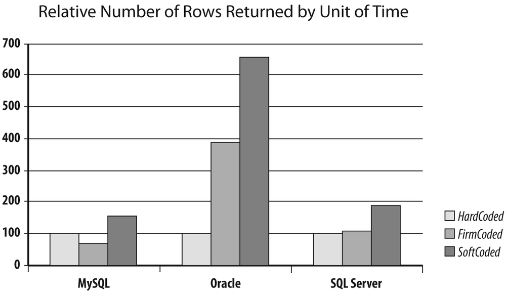
The differences are very interesting to consider, particularly in the case of FirmCoded.java: with Oracle there is a big performance boost, whereas with MySQL there is a noticeable performance penalty. Why is that? Actually, the MySQL Connector/J (the JDBC driver) documentation states that prepared statements are implemented by the driver and the same documentation makes a difference between client-side prepared statements and server-side prepared statements. It is not, actually, a language or driver issue: I rewrote all three programs in C, and although everything ran faster than in Java, the performance ratio was strictly identical among HardCoded, FirmCoded, and SoftCoded. The difference between MySQL and Oracle lies in the way the server caches statements. MySQL caches query results: if identical queries that return few rows are executed often (which is typically the pattern we can see on a popular website that uses a MySQL-based content management system, or CMS), the query is executed once, its result is cached, and as long as the table isn’t modified, the result is later returned from the cache every time the same query is handed to the server. Oracle also has a query cache, although it has been introduced belatedly (with Oracle 11g); however, for decades it has used a statement cache, where execution plans, instead of results, are saved. If a similar (byte for byte) query has already been executed against the same tables and is still in the cache, it is reused even by another session as long as the environment is identical.[16]
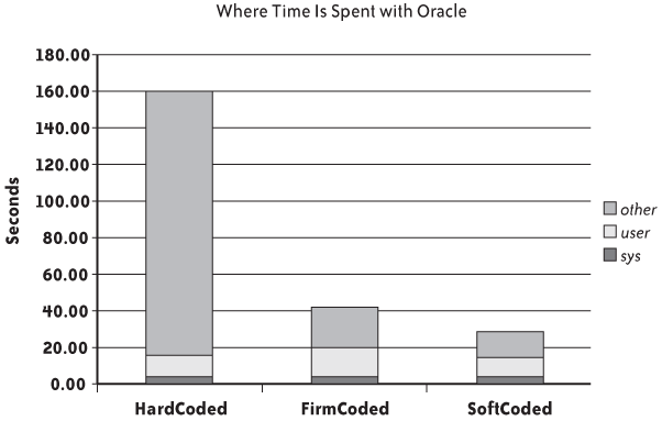
With Oracle, each time a new query is passed to the server, the query is checksummed, the environment is controlled, and the cache is searched; if a similar query is found, we just have this “soft parse” and the query is executed. Otherwise, the real parsing operation takes place and we have a costly “hard parse.” In FirmCoded, we replace hard parses with soft parses, and in SoftCoded we get rid of soft parses altogether. If I run the various programs through the Unix time command, as I did in Figure 2-2, I can see that the difference in elapsed time takes place entirely on the server side, because CPU consumption on the client side (the sum of sys and user) remains more or less the same. Actually, because FirmCoded executes multiple allocations and de-allocations of a prepared statement object, it is the program variant that consumes the most resources on the client side.
By contrast, with MySQL when we prepare the statement we associate it with a particular plan, but if the query cache is active (it isn’t by default), the checksumming takes place after parameters have been substituted to see whether the result can be fetched from the cache. And as long as the bind variables are different, a statement that is “prepared” is hard-parsed. As a result, in FirmCoded, where statements are prepared to be executed only once, there is no performance benefit at all. We plainly see the performance penalty due to a costlier client side. As soon as the statement is reexecuted with different values, as is the case with SoftCoded, the link between the statement to run and its execution plan is preserved, and there is a significant performance benefit, if not quite as spectacular as with Oracle.
SQL Server lies somewhere in between, and even if in the light of results it looks closer to MySQL than to Oracle, its internal mechanisms are actually much closer to Oracle (execution plans can be shared). What blurs the picture is the fact that, on as simple a query as in my example, SQL Server performs simple parameterization of the hardcoded statement—when it analyzes a hardcoded statement and if it looks safe enough (with a primary key, it’s pretty safe), the DBMS just rips the constant off and passes it as a parameter. In the case of SQL Server, the hardcoded statements were, through internal DBMS mechanisms, transmogrified into something similar to the prepared statements of FirmCoded.java; as a result, the original performance was in fact much better than with Oracle. FirmCoded.java was slightly better, though, because each time we prepared the statement, we saved that additional processing of ripping constant values off before checking whether the statement had already been executed. I should emphasize, though, that simple parameterization is not performed aggressively, but quite the contrary, and therefore it “works” in only simple cases.
The first (and intermediate) conclusion is that hardcoding statements borders on the suicidal with Oracle, is to be avoided with SQL Server, and inflicts a severe performance penalty on any DBMS whenever a single session repeatedly runs statements that have the same pattern.
Somehow, using prepared statements with Oracle and with SQL Server is altruistic: if all sessions use prepared statements, everyone benefits, because only one session will go through the hard parse. By contrast, with MySQL it’s a more selfish affair: one session will significantly benefit (50% in my example) if it reexecutes the same query, but other sessions will not. Beware that I am talking here of database sessions; if you are using an application server that pools several user sessions and you make them share a smaller number of database sessions, user sessions may mutually benefit.
Correcting Parsing Issues
Even developers with some experience often end up hardcoding statements when their statements are dynamically built on the fly—it just seems so natural to concatenate values after concatenating pieces of SQL code.
First, when you concatenate constant values, and particularly strings entered into web application forms, you’re taking a huge risk if you’re not extra careful (if you’ve never heard SQL being associated with injection, it is more than time to use your favorite web search engine).
Second, many developers seem to believe that hardcoding a statement doesn’t make much difference when “everything is so dynamic,” especially as there are practical limits on the number of prepared statements. But even when users can pick any number of criteria among numerous possibilities, the number of combinations can be big (it’s 2 raised to the power of the number of criteria), but wide arrays of possible combinations are usually compounded by the fact that some combinations are extremely popular and others are very rarely used. As a result, the real diversity comes from the values that are entered and associated to a criterion, much more than from the choice of criteria.
Switching from hardcoded to "softcoded” statements doesn’t usually require much effort. When using a prepared statement, the previous code snippet for the hardcoded statement appears as follows:
      start = System.currentTimeMillis();
      try {
           long      txid;
           float     amount;
           PreparedStatement st = con.prepareStatement("select amount"
                                                     + " from transactions"
                                                     + " where txid=?");
           ResultSet rs;

           for (txid = 1000; txid <= 101000; txid++){
              st.setLong(1, txid);
              rs = st.executeQuery();
              if (rs.next()) {
                 amount = rs.getFloat(1);
              }
           }
           rs.close();
           st.close();
      } catch(SQLException ex){
            System.err.println("==> SQLException: ");
            while (ex != null) {
                System.out.println("Message:   " + ex.getMessage ());
                System.out.println("SQLState:  " + ex.getSQLState ());
                System.out.println("ErrorCode: " + ex.getErrorCode ());
                ex = ex.getNextException();
                System.out.println("");
            }
      }
      stop = System.currentTimeMillis();
      System.out.println("SoftCoded - Elapsed (ms)	" + (stop - start));
Modifying the code is very easy when, as in this case, the number of values to “parameterize” is constant. The difficulty, though, is that when statements are dynamically built, usually the number of conditions varies, and as a matter of consequence the number of candidate parameters varies with it. It would be very convenient if you could concatenate a piece of SQL code that contains a place marker, bind the matching variable, and go on your way. Unfortunately, this isn’t how it works (and you would run into difficulties when reexecuting the statement, anyway): the statement is first prepared and then the values bound to it, but you cannot prepare the statement before it is fully built.
However, because the building of a statement is usually directed by fields that were entered by a user, it isn’t very difficult to run twice through the list of fields—once to build the statement with placeholders and once to bind the actual values to placeholders.
Replacing hardcoded statements with softcoded statements isn’t an enormous rewriting effort, but it isn’t something you can do mechanically either, which is why people are often tempted by the easiest solution of letting the DBMS do the job.
Correcting Parsing Issues the Lazy Way
You have seen that SQL Server attempts to correct parsing issues on its own. This attempt is timid, and you can make it much more daring by setting the database PARAMETERIZATION parameter to FORCED. As you might have expected, an equivalent feature exists in Oracle with the CURSOR_SHARING parameter, the default value of which is EXACT (i.e., reuse execution plans only when statements are strictly identical), but can be set to SIMILAR (which is very close to the default value of SIMPLE for the SQL Server PARAMETERIZATION parameter) or to FORCE. There are, though, a number of minor differences; for instance, the parameter can be set with Oracle either database-wide[17] or within the scope of a session. Oracle also behaves slightly more aggressively, when asked to do so, than SQL Server. For instance, SQL Server would leave the following code snippet alone:
and char_column like 'pattern%'
whereas Oracle will turn it into this:
and char_column like :"SYS_B_n" || '%'Similarly, SQL Server will leave a statement that already contains at least a single parameter to its own destiny, whereas Oracle will happily parameterize it further. But by and large, the idea behind the feature is the same: having the DBMS do what developers should have done in the first place.
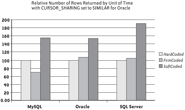
I ran my tests a second time with Oracle, after executing (with the privileges of a database administrator) the following command:
alter system set cursor_sharing=similar;
As I indicated, this setting instructs Oracle to behave as SQL Server does without having to be told. And if I replace the figures previously obtained with Oracle with the new result, I get improvement ratios that are much more in line with what we got with SQL Server, because for both SQL Server and Oracle, if statements are still hardcoded in the program in HardCoded.java, they are no longer hardcoded when they are executed (see Figure 2-3).
From a practical point of view, if we are running on Oracle and we notice parsing issues, one of our first sanity checks should be to verify the setting of the cursor_sharing parameter and, if it happens to be exact, to set it to similar and examine whether it improves performance.
Correcting Parsing Issues the Proper Way
Why bother (besides to protect against SQL injection) with using prepared statements if the DBMS can do it for us? First, we can see with both the Oracle and SQL Server examples that if the automated parameterization process is only slightly less efficient than prepared statements, statements that are prepared once and are executed many times are at least 1.5 times faster than statements that are parameterized before each execution. Second, having AutoCorrect under the Tools option of the menu bar in your word processor doesn’t mean you should happily ignore grammar and let auto-correction go amiss. Third, the less aggressive type of system-enabled parameterization errs on the side of caution and will, with real-world applications, alleviate only some of the pain; the more aggressive type can throw you into deep trouble.
You should be careful not to replace every constant with a place marker. When you have a column with a low cardinality (i.e., a small number of different values), passing the values at runtime can actually be harmful if the values are not uniformly distributed; in plain English, you can have bad surprises if one value is very common and the others are comparatively rare (a common occurrence with columns that record a status). The case when it hurts is when the column with few values is indexed because the rare values are extremely selective. When the optimizer decides what the best execution plan is likely to be, and if, when scanning the statement, it encounters something such as the following:
and status = ?
and if the status column is indexed, it has to decide whether it should be using this index (possibly giving it preference over another index). In a join, it can influence the decision of visiting the table to which status belongs before others. At any point, the goal of the optimizer is to funnel what will become the result set as quickly as possible, which means filtering out the rows that cannot possibly belong to the result set as early as possible.
The problem with place markers is that they provide no clue about the actual value that will be passed at runtime. At this stage, there are several possibilities, which depend on what the optimizer knows about the data (statistics that are often routinely collected as part of database administration):
No statistics have ever been collected, and the optimizer knows nothing at all about what the column contains. In that case, the only thing it knows is that the index isn’t unique. If the optimizer has the choice between a nonunique index and a unique index, it will prefer the unique index because one key value can, at most, return one row with a unique index. If the optimizer only has a choice between nonunique indexes, it depends on your luck.[18] Hence, the importance of statistics.
Statistics are not extremely precise, and all the optimizer knows is that the column contains few distinct values. In such a case, it will generally ignore the index, which can be quite unfortunate when the condition on
statushappens to be most selective.Statistics are precise, and the optimizer also knows, through frequency histograms, that some values are very selective and others are not selective at all. When confronted with the place marker, the optimizer will have to choose from the following:
— Unbridled optimism, or assuming that the value that is passed will always be very selective, and therefore, favoring an execution plan that gives preeminence to the condition on
status. In spite of the nice alliteration, you are unlikely to meet optimistic optimizers, because optimism can backfire.— Playing it safe, which means ignoring the index, because statistically, it is likely to be of dubious use. We are back to the case where the optimizer knows only that there are few distinct values and nothing else, and once again, this may be the wrong tactic when the condition on
statushappens to be the most selective one in the query.— Being clever, which means indiscreetly peeping at the value that is passed the first time (this is known as bind variable peeking with Oracle). If the value is selective, the index will be used; if not, the index will be ignored. This is all very good, but what if in the morning we use selective values, and then the pattern of queries changes during the day and we end up querying with the most common value later on? Or what if the reverse occurs? What if for some reason a query happens to be parsed again, with values leading to a totally different execution plan, which will be applied for a large number of executions? In that case, users will witness a seemingly random behavior of queries—sometimes fast and sometimes slow. This is rarely a popular query behavior with end-users.
— Being even cleverer and, knowing that there may be a problem with one column, checking this column value each time (in practice, this means behaving as though this value were hardcoded).
As you see, place markers are a big problem for optimizers when they take the place of values that are compared to indexed columns containing a small number of unevenly distributed values. Sometimes optimizers will make the right choice, but very often, even when they try to be clever, they will make the wrong bet, or they will select in a seemingly erratic way a plan that may in some cases stand out as very bad.
For low-cardinality columns storing unevenly distributed values, the best way to code, if the distribution of data is reasonably static and there is no risk of SQL injection, is by far to hardcode the values they are compared to in a where clause. Conversely, all uniformly distributed values that change between successive executions must be passed as arguments.
Handling Lists in Prepared Statements
Unfortunately, one case occurs often (particularly in dynamically built statements) but is particularly tricky to handle when you are serious about properly preparing statements: in (…) clauses, where the … is a comma-separated list, not a subquery.
In some cases, in clauses are easy to deal with:
When we are checking a status column or any column that can take one of a few possible values, the
inclause should stay hardcoded for the same reason you just saw.When there is a high variability of values, but when the number of items in the list is constant, we can easily use prepared statements as usual.
The difficulty arises when the values vary wildly, and the number of items in the list varies wildly, too. Even if you use prepared statements and carefully use markers for each value in the list, two statements that differ only in terms of the number of items in the list are distinct statements that need to be parsed separately. With prepared statements, there is no notion of the “variable list of arguments” that some languages allow.
Lists wouldn’t be too much of an issue if all you had was a single condition in the where clause with an in criterion taking its values from a drop-down box in an HTML form; even if you can select multiple entries, the number of items you may have in your list is limited, and it is not a big deal to have, say, 10 different statements in the cache: one for a single-value list, one for a two-value list, and so on up to a 10-value list.
But now suppose that this list is just one out of five different criteria that can be dynamically added to build up the query. You must remember that having five possible criteria means we can have 32 (25) combinations, and having 32 different prepared statements is perfectly reasonable. But if one of these five criteria is a list that can take any number of values between 1 and 10, that list is, by itself, equivalent to 10 criteria, and our five criteria are actually equivalent to 14. As such, 214 = 16,284, and we no longer are in the same order of magnitude as before. And of course, the bigger the maximum possible number of items in the list, the worse the number of combinations. Possibilities explode, and the benefit of using prepared statements dwindles.
With this in mind, there are three ways to handle lists in prepared statements, and I discuss them in the next three subsections.
Passing the list as a single variable
By using some tricky SQL, you can split a string and make it look like a table that can be selected from or joined to other tables later. To explain further I will use a simple example in MySQL that you can easily adapt to another SQL dialect. Suppose our program is called by an HTML form in which there is a drop-down list from which you can select multiple values. All you know is that 10 values, at most, can be returned.
The first operation is to concatenate all selected values into a string, using a separator (in this case, a comma), and to both prefix and postfix the list with the same separator, as in this example:
',Doc,Grumpy,Happy,Sneezy,Bashful,Sleepy,Dopey,'
This string will be my parameter. From here, I will multiply this string as many times as the maximum number of items I expect, by using a Cartesian join as follows:
select pivot.n, list.val
from (select 1 as n
      union all
      select 2 as n
      union all
      select 3 as n
      union all
      select 4 as n
      union all
      select 5 as n
      union all
      select 6 as n
      union all
      select 7 as n
      union all
      select 8 as n
      union all
      select 9 as n
      union all
      select 10 as n) pivot,
    (select ? val) as list;
There are several ways to obtain something similar to pivot. For instance, I could use an ad hoc table for a larger number of rows. If I substitute the string to the placeholder and run the query, I get the following result:
mysql> . list0.sql
+----+------------------------------------------------+
| n  | val                                            |
+----+------------------------------------------------+
|  1 | ,Doc,Grumpy,Happy,Sneezy,Bashful,Sleepy,Dopey, |
|  2 | ,Doc,Grumpy,Happy,Sneezy,Bashful,Sleepy,Dopey, |
|  3 | ,Doc,Grumpy,Happy,Sneezy,Bashful,Sleepy,Dopey, |
|  4 | ,Doc,Grumpy,Happy,Sneezy,Bashful,Sleepy,Dopey, |
|  5 | ,Doc,Grumpy,Happy,Sneezy,Bashful,Sleepy,Dopey, |
|  6 | ,Doc,Grumpy,Happy,Sneezy,Bashful,Sleepy,Dopey, |
|  7 | ,Doc,Grumpy,Happy,Sneezy,Bashful,Sleepy,Dopey, |
|  8 | ,Doc,Grumpy,Happy,Sneezy,Bashful,Sleepy,Dopey, |
|  9 | ,Doc,Grumpy,Happy,Sneezy,Bashful,Sleepy,Dopey, |
| 10 | ,Doc,Grumpy,Happy,Sneezy,Bashful,Sleepy,Dopey, |
+----+------------------------------------------------+
10 rows in set (0.00 sec)
However, there are only seven items in my list. Therefore, I must limit the number of rows to the number of items. The simplest way to count the items is to compute the length of the list, remove all separators, compute the new length, and derive the number of separators from the difference. Because by construction I have one more separator than number of items, I easily limit my output to the right number of rows by adding the following condition to my query:
where pivot.n < length(list.val) - length(replace(list.val, ',', ''));
Now, I want the first item on the first row, the second item on the second row, and so on. If I rewrite my query as shown here:
select pivot.n, substring_index(list.val, ',', 1 + pivot.n)
from (select 1 as n
      union all
      select 2 as n
      union all
      select 3 as n
      union all
      select 4 as n
      union all
      select 5 as n
      union all
      select 6 as n
      union all
      select 7 as n
      union all
      select 8 as n
      union all
      select 9 as n
      union all
      select 10 as n) pivot,
    (select ? val) as list
where pivot.n < length(list.val) - length(replace(list.val, ',', ''));
I get the following result with my example string:
mysql> . list2.sql
+----+------------------------------------------------+
| n | substring_index(list.val, ',', 1 + pivot.n)     |
+----+------------------------------------------------+
| 1 | ,Doc                                            |
| 2 | ,Doc,Grumpy                                     |
| 3 | ,Doc,Grumpy,Happy                               |
| 4 | ,Doc,Grumpy,Happy,Sneezy                        |
| 5 | ,Doc,Grumpy,Happy,Sneezy,Bashful                |
| 6 | ,Doc,Grumpy,Happy,Sneezy,Bashful,Sleepy         |
| 7 | ,Doc,Grumpy,Happy,Sneezy,Bashful,Sleepy,Dopey   |
+----+------------------------------------------------+
7 rows in set (0.01 sec)
I am very close to the final result, which I obtain by applying substring_index() a second time. I want substring_index() to now return the last item in each row, which I make it do by replacing the first line in my query with this:
select pivot.n,
       substring_index(substring_index(list.val, ',', 1 + pivot.n), ',', -1)
This gives me the following:
mysql> . list3.sql
+---+-----------------------------------------------------------------------+
| n | substring_index(substring_index(list.val, ',', 1 + pivot.n), ',', -1) |
+---+-----------------------------------------------------------------------+
| 1 | Doc                                                                   |
| 2 | Grumpy                                                                |
| 3 | Happy                                                                 |
| 4 | Sneezy                                                                |
| 5 | Bashful                                                               |
| 6 | Sleepy                                                                |
| 7 | Dopey                                                                 |
+---+-----------------------------------------------------------------------+
7 rows in set (0.00 sec)

mysql>
As you may have noticed, although the query is more complicated than the average SQL textbook query, it works as shown here with any list that contains up to 10 items, and can be easily accommodated to handle bigger lists. The text of the statement remains identical and will not be reparsed, even when the number of items in the list changes.
Passing list values as a single string is a very good and efficient solution for small lists. Its limitation is the length of the character string: you may hit a constraint either in the wrapper language or in SQL (Oracle has the shortest limit, at 4,000 characters); if your list contains several hundred items, another solution may be more appropriate.
Batching lists
One solution is to operate by batches, trying to keep lists to a fixed number of items. What allows us to use such a method is the fact that in() ignores duplicates in the list, whether it is an explicit list or the result of a subquery. Suppose we get our parameters in an array that, as in the previous example, can contain up to 10 values. If I try to softcode the statement, I may write something such as this:
my_condition = "where name in"
loop for i in 1 to count(myarray)
     if i > 1 then my_condition = my_condition + "("
                  else my_condition = my_condition + ","
    my_condition = my_condition + "?"
end loop
my_condition = my_condition + ")"
Then I’ll loop again to bind each value to its place marker, and I’ll get as many different statements as I may have items in the list. What I can do instead is build a statement that can handle up to 10 items in the list:
my_condition = "where name in (?,?,?,?,?,?,?,?,?,?)"
Then I can prepare the statement by executing the suitable database call, and systematically bind 10 parameters by repeating some of the actual parameters to complete the 10 items:
loop for i in 1 to 10
     j = 1 + modulo(i, count(array))[19]
     bind(stmt_handler, i, array(j))
end loop
If need be, we can have several list sizes, with one statement to accommodate, say, lists with from 1 to 20 items, another statement for lists with from 21 to 40 items, and so on. This way, when we get lists containing any number of items up to 100, we are sure to keep in the cache, at most, 5 different statements instead of 100.
Using a temporary table
With very large lists, the simplest solution is probably to use a temporary table, and to replace the explicit list with a subquery that selects from this temporary table—once again, the text of the query will remain the same regardless of the number of rows in the temporary table. The downside to this method is the cost of insertion: it adds more interaction with the database. However, the real question concerns the origin of the data that is used to populate the list. For huge lists, it’s not unusual for the items to come from a query. If this is the case, insert … select … into a temporary table will take place entirely on the server, and will save fetching the data into the application program. At this point, you may be wondering whether a temporary table is really necessary, and whether a simple subquery or join wouldn’t do the trick much more efficiently. If the data comes from an external file and if this file can be sent to the server that hosts the database, you can use various utilities to load a temporary table almost painlessly. (Oracle’s external tables, MySQL’s load data infile statement, and SQL Server Integration Services all provide developers with tools that can eliminate a lot of programming.)
Bulk Operations
Besides indexing, statistics, and parsing rate, which are general points affecting one particular application or all applications accessing the database, there are other types of processes that you should check when performance isn’t as good as expected. For instance, one factor that can slow down performance considerably when fetching (or inserting) a large number of rows is the number of round trips, particularly when there is a wide area network (WAN) between the application server and the database (yes, it happens).
Unfortunately, I am touching on a topic that is dependent not only on the DBMS, but also on the language that is used to access that DBMS. I am therefore going to give a broad sketch to point at possible issues and give some examples. The principle is very simple: suppose you have to move a heap of sand. Operating row by row is like moving the heap of sand with a teaspoon. Perhaps using a shovel or a wheelbarrow would be more efficient.
Implementations vary. Some leave more to the imagination than others, but in all cases, when you fetch data from a server in a cursor loop you issue calls that say, in effect, “send me more data.” At a very low level, you send on the network a packet that contains this command. In return, the DBMS sends back another packet that either contains the data you require or simply says “I’m done.” Each time, you have a round trip and, as a matter of consequence, some network latency. The same types of exchanges occur when you insert row after row of data. Packets that are exchanged have a fixed size, and sending a full packet is neither more expensive nor slower than sending a mostly empty packet; exchanging fuller packets will mean fewer exchanges for the same amount of data. When you insert or return massive amounts of data—for instance, to create a file that is to be sent elsewhere for further processing by another system—it makes little sense to send row after row to the server, or to fetch row after row from the server, even when the procedural part of your program actually processes one row at a time. Some products and programmatic environments allow you to batch operations; this is typically the case with, for instance, T-SQL, JDBC, and SQLJ, which allow you to group several insert statements before sending them to the server, or the SqlPipe object in the .NET Framework. Others allow you to insert from or fetch into arrays, as is the case with Oracle and PL/SQL or the OCI C/C++ interface. MySQL takes a slightly different approach with streaming; it sends an uninterrupted flow of data without being explicitly prompted for it. If you use the C or PHP libraries, for instance, you will get the entire result set at once, which is fine for a small to moderately sized result set, but may lead to memory shortages when you really need to return a lot of data, in which case you must switch to another mode.
In some cases, batching is implicitly performed by the client side of your application. For instance, you may code this:
while fetch_one_row_from_database()
       do something
and behind your back the client side performs this:
while fetch_one_row_from_array()
      do something

fetch_one_row_from_array {
     increase index;
     if index > array_size
            fetch_array_size_rows_at_once_from_database
            set index to point to first array entry
     if buffer[index] is empty
           return done
    else
           return buffer(index)
This is typically what can happen in a JDBC program, in PHP database interface functions, or in some C/C++ client libraries. What few developers remember is that the array size is sometimes under their control, and that the default value isn’t always the most suitable for what they have to do.
Figure 2-4 shows how performance is affected by setting the “fetch size” in the case of a JDBC program that dumps the contents of the transactions table used in Chapter 1 to a CSV file. Don’t try to compare the various products with one another because all tests weren’t run on the same machine, and I have normalized the number of rows returned by unit of time into a “throughput index.” MySQL and SQL Server (i.e., their JDBC drivers) clearly ignore the settings, but Oracle is extremely sensitive to the parameter. Increasing the fetch size from its default value of 10 to 100 doubles the throughput on this example with very little effort (and both the JDBC program and the database were running on the same machine). When I wrote that MySQL ignores the settings, that was not quite true: I was able to push the MySQL throughput by about 15% by creating the statement of type forward only and read only, and by setting the fetch size to Integer.MIN_VALUE, which triggered a switch to a faster (in that case) streaming mode (which happens to also be supported by SQL Server’s TDS protocol).
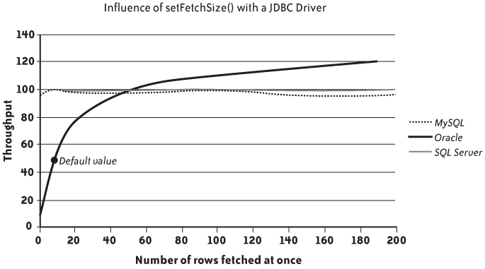
All the cases I have mentioned so far take a rather conservative approach to bulk operations, by mostly buffering data to optimize transfers. You may also encounter bulk operations that go beyond buffering and boldly bypass regular SQL operations, which for massive processes can also be very interesting: for instance, bulk copy operations with SQL Server’s SQL Native Client, or the direct path-loading functions of Oracle’s C call interface. But in that case, we are very far from quick, simple changes.
Transaction Management
Another important point to check is how transactions are managed. Transactions are supposed to be a break-or-pass suite of statements, opened either implicitly by the first statement that changes the database, or explicitly, and ended with either a commit, which makes the change permanent if the server were to crash, or a rollback, which cancels all changes to the database since the beginning of the transaction (or an optional, intermediary savepoint). The end of the transaction releases the locks acquired by the session on the table, page, or row that was changed, depending on the grain of locking. In practice, if the server crashes in the middle of a transaction, any changes are lost because they were not necessarily written to disk (if they were, they will be rolled back when the database starts).
Committing takes time, because the only way to ensure that the changes will be permanent—even if the database crashes—is to record all updates to a file in nonvolatile memory, and not to return before the data is actually written. Commit changes very often, and you’ll realize that a significant part of your time is taken up by these waits.
Committing often is critical in online transaction processing (OLTP) environments, because if locks are held for longer than necessary, concurrent transactions are serialized and pile up, waiting for the previous transaction to complete and unlock the resource. It’s somewhat different during nightly batch updates when there is no concurrency and one process inserts, purges, or updates data on a grand scale. If you are unsure about how often your data loading or upgrading batch program commits in the course of its run, this is definitely a point to check. The default with some languages (hi, JDBC!) is to be in a so-called "auto-commit” mode—that is, to commit after every change to the database, which, as Figure 2-5 shows, is extremely painful to all database products. (I normalized the number of rows updated by unit of time in a massive update to two million rows.)
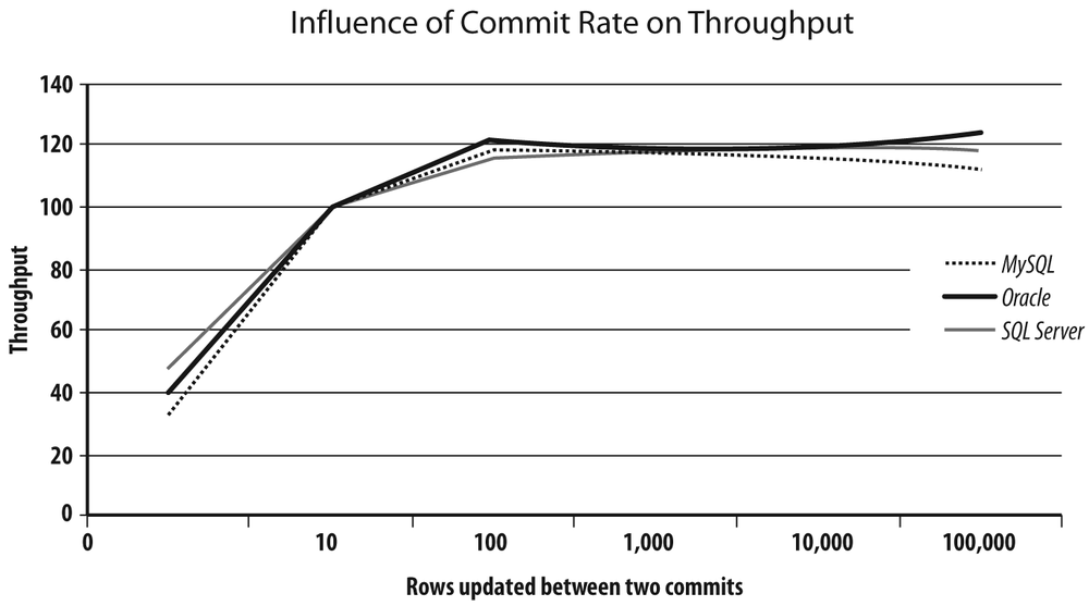
I should add that when you are operating in auto-commit mode, you are not only severely impairing your batch programs, but also sacrificing the concept of transactions, because the logical unit of work becomes the SQL statement. This can present some interesting situations. Suppose you want to transfer money from your checking account to your savings account. First you update your checking account to subtract the amount you want to transfer, and then update your savings account to add that same amount. Now picture a computer crash between the two updates. Oops. That’s what transactions were invented for: if the two updates are in the same transaction, the first update will be canceled. If not, expect to spend some time on the phone with your bank.
We will return to transaction and commit frequency in Chapter 6, but as far as “quick wins” are concerned, this is all I will say on this topic for the moment. It is now time to take a look at views and stored functions.
[10] Only regular indexes, not clustered indexes.
[11] Which may hint at an uncertain table design.
[12] I don’t want to get into the gory details about index structure; suffice it to say that B-trees are tree structures like any hierarchical structure you can think of, except that they are primarily designed to be self-reorganizing and to grow slowly in depth. Moreover, search times are identical for all keys.
[13] In some rare cases, primary key constraints may be enforced using a nonunique index.
[14] Full-text indexes are an integral part of SQL Server and MySQL, and they are available, although not as closely integrated, with Oracle.
[15] Both muses (lesser goddesses) of poetry in Greek mythology.
[16] A session can locally tweak some parameters that affect the way a statement will be executed.
[17] Don’t forget that database doesn’t mean the same as in the SQL Server and MySQL worlds, where you would talk of a server.
[18] All right, luck can sometimes be helped.
[19] The first value will not be the first entry in the array, but it works fine nevertheless.