
Chapter 7. Refactoring Flows and Databases
Diseases desperate grown By desperate appliance are relieved, Or not at all.
—William Shakespeare (1564–1616)
Hamlet, IV, 3
SO FAR, I HAVE FOCUSED ON IMPROVING CODE AND MAKING BETTER USE OF THE DBMS FROM A UNITARY standpoint. Not unitary as in “single row,” but unitary as in “single instance of the program.” With the possible exception of some critical batch programs, rarely does a program have exclusive access to a database; most often, multiple instances of the same program or different programs are querying and updating the data concurrently. Ensuring that programs are as efficient and as lean as time, budget, and the weight of history allow is a prerequisite to their working together efficiently. You will never get a great orchestra by assembling bad musicians, and very often one bad musician is enough to ruin the whole orchestra. Bringing together virtuosi is a good start, but it’s not everything. I won’t spoil much by saying that if you replace a complex game of ping-pong between a program and the DBMS with efficient operations, you are in a better position to gear up. Yet, scalability issues are complex, and there is more to orchestrating a harmonious production than improving the performance of processes that run alone, because more points of friction will appear. I briefly mentioned contention and locking in previous chapters, but I didn’t say much about environments where there is intense competition among concurrent users. In these environments, laissez faire often makes bottlenecks turn to strangleholds, and you need to regulate flows when concurrency dramatically degrades performance.
In turn, diminishing contention often requires changes to either the physical or the logical structure of the database. It is true that good design is one of the main factors defining performance. But refactoring is an activity that operates in a sort of last-in, first-out fashion: you start with what came last in the development process, and end with what came first. Unfortunately, when you are called in for refactoring, databases have usually been in production for quite a while and are full of data. Reorganizing the databases isn’t always a viable option, even when the logical structure is untouched, simply because you cannot afford the service interruption that results when transferring the data, rebuilding the indexes, and deactivating and reactivating integrity constraints (which can take days, literally), or simply because management feels rather chilly about the business risk involved. It’s even worse when physical alterations come along with changes to the logical view that will require program changes, as is usually the case. It’s always better to plan for the basement garage before you build the house; moreover, the costs of digging that basement garage after the building is complete aren’t exactly the same for a one-story suburban house as they are for a skyscraper. Sometimes tearing everything down and rebuilding may be cheaper. With a database, an operation as simple as adding a new column with a default value to a big table can take hours, because data is organized as rows (at least with the best-known DBMS products) and appending data to each row requires an enormous amount of byte shifting. [47]
With that being said, when business imperatives don’t leave much leeway for organizing processes, reviewing the organization of the database may be your last card to play. This chapter expands on the topics of concurrent access and physical reorganization.
Reorganizing Processing
In Chapter 1, I advised you to try to monitor queries that the DBMS executes. You may be surprised by what you find, and you may see that queries that are fairly innocent when considered alone may not be so innocent when considered as a herd. For instance, you may discover costly hardcoded queries that different sessions execute several times in a brief period and are unlikely to return a different result each time. Or you may discover that the application side of this time-tracking package happily loads (through a series of select * from … without any where clause) the entire table that stores employees and the entire table that references tasks each time someone connects to report what he or she has been doing during the week. [48] It never hurts to ask innocently whether a query actually needs to be run that number of times, and if so, whether it is possible to store the result set to some temporary area so that only the first session runs the expensive query and the others just retrieve the result from a cache. Or whether, instead of loading all the necessary data at once, it would be a better idea to limit oneself to data that is always required and to introduce some “load-on-demand” feature for whatever doesn’t fall into the previous categories. People who write functional specs usually think “one program instance.” By raising a number of questions and suggesting alternative possibilities to people who know the functional side very well, you will not necessarily find a suitable solution on your own, but very often you will trigger a discussion from which many ideas for improvement will emerge.
Competing for Resources
When dealing with databases and concurrency, the best model to keep in mind is one or several service providers, with a number of requesters trying to obtain the service, as shown in Figure 7-1. The issue is that whenever one requester is being serviced, others usually have to wait.
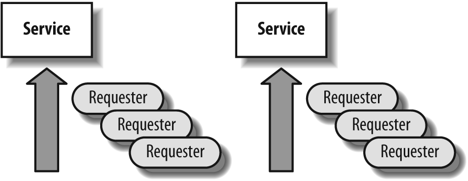
This model applies as well to the following:
Low-level resources such as CPU usage, input/output (I/O) operations, or memory areas that need to be written or read
High-level resources such as rows or tables that are locked
The model of the service providers serving requesters that line up (queue) and the ensuing “queuing theory” is very well known and is one of the pillars of software engineering. Beneath the mathematics, it describes situations that are common in real life. If you have to wait for the CPU because your machine is running flat out and if you are certain that you will require most of the CPU cycles, there is no question that you have to upgrade your machine. But often, while lines are accumulating with many requesters waiting for one resource, other service providers within the same system are just idle. For instance, this may happen when your machine is spending a lot of time waiting for I/O operations to complete. The difficulties lie in regulating flows and spreading the load among heterogeneous resources.
Service time and arrival rate
Let’s first consider what happens with a single service provider. In a system based on service providers and requesters, the two values that really matter are how long it takes the service provider to perform its task (the service time) and how fast requesters pop in (the arrival rate). Most important of all is the relationship between these two values.
When the arrival rate, even for a short while, is too high for the service time, you get a lengthening line of requesters waiting to be serviced.
For instance, look at what happens in a currency exchange booth where you have only one employee. If people who want to change their money arrive slowly, and if there is enough time to service one person before someone else arrives, everything is relatively fine. But the real trouble starts when requesters arrive faster than they can be serviced, because they accumulate; imagine that the currency exchange booth is in an airport and that an A380 airplane has just landed ….
There are only a few ways to improve throughput in such a system.
On the service provider side, you can do one of the following:
Try to service the request faster by doing exactly the same thing at a faster pace.
Add more employees to provide the same service. This method works great if there is no interaction among the employees—for instance, if each employee has a stack of banknotes in various currencies and can change money independently from the others. This method will work very poorly if all the employees need to get exclusive access to a shared resource—for instance, if they are instructed to take a photocopy of passports, and if there is only one photocopier for all employees. In that case, the bottleneck will be access to the photocopier; customers will feel that they wait for the employee, when in reality they are waiting for the photocopier. However, having more employees may only be beneficial when there is some overlap between the employees’ activities: if while one employee photocopies passports another one is collecting them from new customers, while a third is counting banknotes and a fourth is filling a slip, global throughput will be far superior to the case when only one employee is active. Nevertheless, the increase in capacity will soon be limited, and before long, adding more employees will simply mean more employees waiting for the photocopier.
On the requester side, you can do one of the following:
Express your requests better so as to get an answer faster.
Try to organize yourself better so as to avoid long lines. For instance, if you take your children to a theme park and find the line at one attraction discouragingly long, you will go elsewhere and try to come back when the line is shorter.
If the request happens to be an SQL query, providing a faster response to the same request is the domain of tuning, and when tuning fails or isn’t enough, faster hardware. Expressing requests better (and getting rid of unnecessary requests such as tallies) was the topic of the two previous chapters. The other two points—increasing parallelism and trying to distribute the load differently in time rather than in space—may present some refactoring opportunities. Unfortunately, you often have much less elbow room in these scenarios than when you are refactoring queries or even processes. It is rare that you cannot improve a slow query or process. But not every process lends itself to parallelism; for instance, nine women will not give birth to a baby after one month of pregnancy.
As such, the performance gain brought by parallelism doesn’t come from one task being shared among several processes, but rather from many similar tasks overlapping. When they reached Spain in 1522 after having sailed around the globe, Magellan’s companions reported that the ruler of Jailolo, one of the Moluccan Islands, had 600 children; it didn’t take him 5,400 months (that’s 450 years) to father them, but having 200 wives definitely helped.
Increasing parallelism
There are several ways to increase parallelism, directly or indirectly: when a program performs a simple process, starting more instances of this program can be a way to increase parallelism (an example follows); but, adding more processors inside the box that hosts the database server or the application server can also serve the same kind of purpose in a different way. If several levers can, under suitable circumstances, help you increase throughput, they achieve it by pulling different strings:
If you start more instances of the same program on the same hardware, it’s usually because no low-level resource (CPU, I/O operations) is saturated, and you hope to make better use of your hardware by distributing resources among the different instances of your program. If you discover that one of your programs spends a lot of time waiting for I/Os and nothing can be done to reduce this time, it can make sense to start one or several other instances that will use the CPU in the meantime and help with the work.
If you add more processors or more I/O channels, it usually means (or should mean) that at least one of the low-level resources is saturated. Your aim is, first of all, to alleviate pain at one particular place.
You will need to be very careful about how the various instances access the tables and rows, and ensure that no single piece of work is performed several times by several concurrent instances that are ignorant of one another and that the necessary coordination of programs will not degenerate into something that looks like a chorus line with everyone lifting her leg in sync. If every instance of the program waits for I/O at the same time, parallelism will have succeeded only in making performance worse.
Among prerequisite conditions to efficient parallelism, one finds fast, efficient transactions that monopolize unsharable resources as little as possible. I mentioned in the preceding chapter the fact that replacing a procedural process with a single SQL query has an advantage other than limiting exchanges between the application side and the server side: it also delegates to the database optimizer the task of executing the process as quickly as possible. You saw in Chapter 5 that there were basically two ways to join two tables: via nested loops and via hash joins. [49] Nested loops are sequential in nature and resemble what you do when you use cursor loops; hash joins involve some preparatory steps that can sometimes be performed by parallel threads. Of course, what the optimizer ultimately chooses to do will depend on many factors, including the current version of the DBMS. But by giving the optimizer some control over the process, you keep all options open and you authorize parallelism, whereas when your code is full of loops you prevent it.
Multiplying service providers at the application level
I created a simple test case to show how you can try to parallelize processing by adding more “service providers” within an application. I only used MySQL for this example (because it allows storage engines that have different grains for locking), and I created a MyISAM table. As row-level locking cannot be applied to MyISAM tables, I have a reasonable worst-case scenario.
In many systems, you find tables that are used primarily as a communication channel between processes: some “publisher” processes record into the table tasks to be performed, while some other “consumer” processes read the table, getting a “to-do” list on a first-in, first-out basis, perform the task, and usually write some ending status back into the table when the task is complete (or has failed). I have partly simulated such a mechanism by focusing exclusively on the “consumer” side. I created a table called fifo that looks like this:
mysql> desc fifo;
+--------------+---------------------+------+-----+---------+----------------+
| Field        | Type                | Null | Key | Default | Extra          |
+--------------+---------------------+------+-----+---------+----------------+
| seqnum       | bigint(20) unsigned | NO   | PRI | NULL    | auto_increment |
| producer_pid | bigint(20)          | NO   |     |         |                |
| produced     | time                | NO   |     |         |                |
| state        | char(1)             | NO   |     |         |                |
| consumed     | time                | YES  |     | NULL    |                |
| counter      | int(11)             | NO   |     |         |                |
+--------------+---------------------+------+-----+---------+----------------+
6 rows in set (0.00 sec)
I inserted into this table 300 rows with state R as in Ready and a value of 0 for counter. A consumer gets the value of seqnum for the oldest row in state R. If none is found, the program exits; in a real case, with permanently active publisher processes, it would sleep for a few seconds before polling again. Then the consumer updates the row and sets state to P as in Processing, using the value of seqnum just found; I would have preferred executing a single update, but because I need seqnum to update the row when the task is complete, I have to execute two queries. [50] Then I simulate some kind of processing by sending the program to sleep for a random number of seconds that is designed to average two seconds. Then the program updates the row, setting the state to D for Done, setting a completion timestamp, and incrementing counter by one.
I should add that there is no other index on fifo except for the primary key index on seqnum; in particular, there is no index on state, which means the search for the earliest unprocessed row will translate into a table scan. This indexing pattern is in no way surprising in such a case. Usually, a table that is used to exchange messages between processes contains very few rows at one point in time: if the system is properly tuned, publishers and consumers work at about the same rate, and some kind of garbage collection program removes processed lines on a regular basis. Indexing state would mean adding the cost of maintaining the index when publishers insert new rows, when consumers change the value of the column, and when rows are cleaned up; it might be worth the overhead, but it is very difficult without extensive testing to declare whether, on the whole, an index on state would help. In this case, there is none.
The first version of the program (consumer_naive.c) executes the following SQL statements in a loop:
select min(seqnum) from fifo
where state = 'R';

update fifo
set state = 'P'
where seqnum = ?; /* Uses the value returned by the first query */
… brief nap …
update fifo
set state = 'D', consumed = curtime(), counter = counter + 1
where seqnum = ?;
It uses the default "auto-commit” mode of the MySQL C API, which implicitly turns every update statement into a transaction that is committed as soon as it is executed.
Learning that with an average “processing” time of around two seconds it takes 10 minutes to process the 300 rows of my fifo table should surprise no one. But can I improve the speed by adding more consumers, which would process my input in parallel? This would be a way to solve a common issue in these types of architectures, which is that publishers rarely publish at a smooth and regular rate. There are bursts of activity, and if you don’t have enough consumers, tasks have a tendency to accumulate. As this example shows, getting rid of the backlog may take some time.
When I start 2 consumers it takes five minutes to process all the tasks, with 5 consumers it takes two minutes, with 10 consumers only one minute, with 20 consumers about 35 seconds, and with 50 processes very close to 15 seconds. There is only one major snag: when I check the value of counter, there are a number of rows for which the value is greater than one, which means the row has been updated by more than one process (remember that a process increases counter when it’s done). I ran my test five times with a varying number of parallel consumers. Figure 7-2 shows the average results that I obtained.
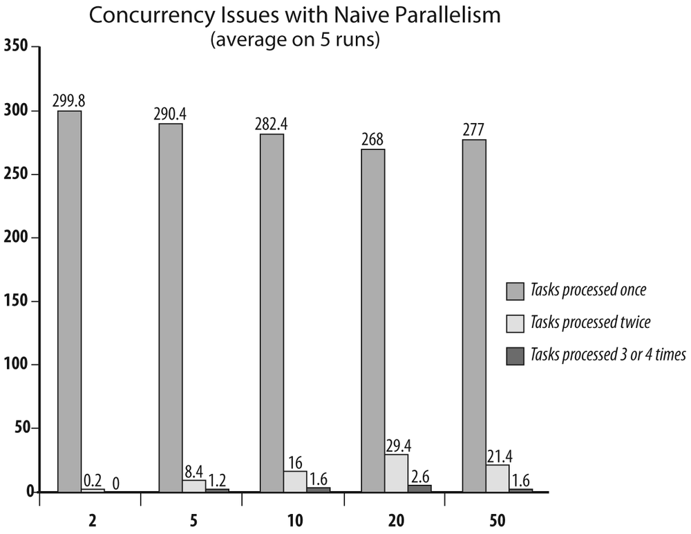
Performing tasks several times isn’t a desirable outcome. Seeing the same debit appear twice on a bank statement would probably not amuse me, no more than discovering that the ticket I bought for a concert or sports event was sold to two or three other people as well.
Parallelism requires synchronization of a sort, and with SQL two elements are involved:
Isolation level defines a session’s awareness of what other concurrent sessions are doing. The ISO standard, which all products more or less support, defines four levels, of which two are of greater practical interest:
- Read uncommitted
In this level, all sessions are instantly aware of what the others are doing. When one session modifies some data, all the other sessions see the change, whether it has been committed or not. This is an extremely dangerous situation, because a transaction can base its own computations on changes that will be rolled back later. You can very easily cause data inconsistencies that will be extremely hard to trace. The only case when you are safe is when you are using auto-commit mode. You can no longer read any uncommitted data, because changes are committed immediately. But auto-commit mode can accommodate only very simple processes.
- Read committed
In this level, a session doesn’t see the changes brought by another session before they are committed. This is similar to what happens when you are using version control software: when a file is checked out, and while someone else is modifying it, you can see only the latest version that was checked in—and you cannot modify it while it is locked. Only when it has been checked in (the equivalent of
commit) will you see the new version. This isolation level is the default for SQL Server.This can be considered a relatively safe isolation level, but it can get you into trouble when you have long-running queries on a table that execute concurrently with very fast updates to that table. Consider the following case: in a bank, you are running an end-of-month query summing up the balance of all of your customers’ accounts. You have many customers, most customers own several accounts, and your
accountstable contains tens of millions of rows. Summing up tens of millions of rows isn’t an instant operation. While your report is running, business carries on as usual. Suppose that an old client, whose current account data is stored “at the beginning of the table” (whatever that means), has recently opened a savings account, the data for which resides toward the end of the table. When your report starts to execute, the current account contains 1,000, and the new savings account contains 200. The report sums up the values, reads 1,000, and proceeds. Soon after the program reads the current account balance, your customer decides to transfer 750 from the current account to the savings account. Accounts are accessed by account numbers (which are the primary keys), the transaction is very fast and is committed immediately, and the savings account is credited 750. But your report program, crunching numbers slowly, is still working on another customer’s account, far away in the table. When the report program finally reaches this particular customer’s savings account, as the transaction was committed many CPU cycles ago, it reads 950. As a result, the sum is wrong.There is a way to avoid this type of issue, which is to require the DBMS to record, at the beginning of a query, some timestamp or functionally equivalent sequence number, and to revert to the version of the data that was current when the query started whenever that query encounters a row that was updated after the reference timestamp. This flashback to the time when the query started occurs whether the change has been committed or not. In the previous example, the program would still read the value 200 for the savings account, because it is the value that was current when the query started. This mechanism is what SQL Server calls row versioning and what it implements with the
READ_COMMITTED_SNAPSHOTdatabase option. This mode happens to be the default mode with Oracle, where it is called read consistency, and is considered to be a variant of the standard read committed isolation level; it is also how the InnoDB storage engine works with MySQL in the read committed isolation level (but it’s not the default level for InnoDB).Of course, there is no such thing as a free lunch, and using row versioning means that old data values must be kept as long as possible instead of being disposed of as soon as the transaction commits. In some environments that combine slow queries and numerous rapidly firing transactions, keeping a long history can lead to excessive usage of temporary storage and, sometimes, runtime errors. There is usually a cap on the amount of storage that is used for recording past values. Uncommitted values are kept until storage bursts at the seams. Committed values are kept as long as possible; then, when storage becomes scarce, they are overwritten by the previous values corresponding to recent changes. If a
selectstatement requires a version of data that was overwritten to accommodate new changes, it will end in error (in Oracle, this is the infamous "snapshot too old” error). Rerunning the statement will reset the reference time and, usually, will lead to successful execution. But when this type of error occurs too often, the first thing to check is whether the statement cannot be made to run faster; if not, whether changes are not committed too often; and if not, whether more storage cannot be allocated for the task.- Repeatable read
The repeatable read isolation level is an extension of row versioning: instead of keeping a consistent view of data for the duration of a query, the scope is the whole transaction. This is the default level with the InnoDB engine for MySQL. With the previous account balance example, if you were to run the query a second time in the repeatable read level, the report program would still see 1,000 in the current account and 200 in the savings account (while in the read committed mode, the report program would read 250 and 950 the second time, assuming that no other transfer has taken place between those two accounts). As long as the session doesn’t commit (or roll back), it will have the same vision of the data that it first read. As you can expect, issues linked to the amount of storage required to uphold past data history are even more likely to occur than in the read committed level.
What can happen, though, is that new rows that have been inserted since the first
selectwill pop up. The read is repeatable with respect to the data that has been read, but not with respect to the table as a whole. If you want the table to look the same between successiveselectstatements, regardless of what happens, you must switch to the next isolation level.- Serializable
This isolation level is a mode in which transactions ignore all the changes brought to the database by the other transactions. Only when the transaction ends does the session see the changes brought to the database by the other sessions since the beginning of the transaction. In a way,
commitdoubles as a refresh button.
In real life, read committed (with or without row versioning) and repeatable read are the only isolation levels that matter in the vast majority of cases. They are the two levels that offer a very consistent view of data without putting too much strain on the system in terms of locks and upkeep of change history.
I just mentioned locks in reference to the various synchronization mechanisms the system maintains on your behalf to keep data consistent. When you define an isolation level, you define, by default, a locking pattern. But you can also explicitly lock tables, to specify to the system that you want exclusive write or, sometimes, read access [51] to one or several tables, and that anyone who will require an access that conflicts with yours after you have grabbed your lock will have to wait until you end your transaction. Conversely, if someone is already accessing the table in a mode that is incompatible with your request when you try to lock the table, your session will have to wait [52] until the other session commits or rolls back its changes.
But let’s return to our MySQL/MyISAM program; we are operating in the default auto-commit mode, and MyISAM allows only one process to update one table at one time. The problem we have (that concurrent processes pounce on the same row) occurs in the phase when we try to grab a row to process—namely, when we execute the following:
select min(seqnum) from fifo
where state = 'R';

update fifo
set state = 'P'
where seqnum = ?;
What happens is that one process gets the identifier of the next row to process, and before it has time to update the table, one or several other processes get the very same identifier. We clearly need to ensure that once we have identified a row as a candidate for processing (i.e., once the select statement has returned an identifier), no other process will get hold of it. Remember that we cannot combine these two statements because we need the identifier to update the row when we are done. A single statement would have fit the bill, because the internal mechanisms of a DBMS ensure the so-called ACID (Atomicity, Consistency, Isolation, Durability) property of a single update statement. (In plain language, you don’t have to worry about a single statement because the DBMS ensures data consistency.)
If we want to run multiple instances of the program and benefit from parallelism, we need to refactor the code once again. One way to do this is to turn off auto-commit mode to get better control of transactions, and then, in the main loop, to lock the table for our exclusive use before we look for the next row to process, update the table, and finally release the lock. At this point, we will be guaranteed to have an ID that we know no other parallel thread will get, and we can feel comfortable knowing that this ID will be processed only once. I used this strategy in my consumer_lock.c program.
Another way to proceed is as follows:
set the number of updated rows to zero
loop
   select min(seqnum) from fifo
   where state = 'R';
   /* Exit if nothing found */
   update fifo
   set state = 'P'
   where seqnum = ?
     and state = 'R';
until the number of updated rows is 1;
When the row is updated, the program checks that it still is in the state where it is expected to be; if the assumption that the row is still in the “Ready” state is not satisfied, it means that another process was quicker to grab it, and we just try to get another row. The algorithm is very close to the original program, except that the update statement is made safe and I have added a provision for failure. I called this program consumer_not_so_naive.c.
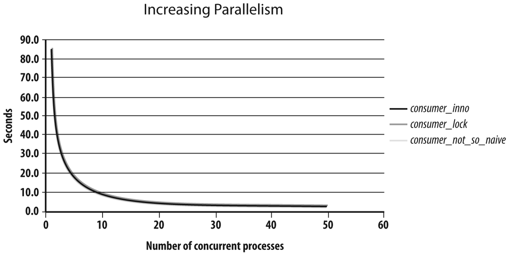
I also wrote another program that uses the “safe update” strategy but also assumes the underlying InnoDB storage engine and the availability of row-level locking. The third program adds the for update clause to the select statement that identifies the next row to process, thus locking the selected row. This program is called consumer_inno.c. I ran all three programs with a pseudobacklog of 200 rows to clear, an average sleep time of 0.4 seconds, and a varying number of concurrent processes between 1 and 50. The results are shown in Figure 7-3. The most outstanding feature of the figure is probably that all three curves overlap one another almost perfectly. All three solutions scale extremely well, and the time that it takes for n processes to clear the backlog is the time it takes one process to clear the backlog divided by n.
You might wonder why it doesn’t make any difference whether we are using table locking or row locking. You mustn’t forget that "service providers” from the application viewpoint are requesters for the database. In this light, there are two very simple reasons why row locking doesn’t perform better than table locking:
The first reason is that all processes are chasing the same row, which is the oldest unprocessed row. For each process, only one row counts, and this row is the critical resource. Whether you are stuck waiting for that row or for the table makes no difference, and row locking brings no measurable benefit in such a case.
The second reason is that even if we have to scan the
fifotable, its modest number of rows makes theselectstatement almost instant. Even when you lock the table for the duration of theselectandupdatestatements, the lock is held for so little time in regard to the “rate of arrival” that waiting lines don’t build up.
Contrary to what you might think, the grain of locks isn’t necessarily the decisive factor in terms of performance on relatively small tables (i.e., up to thousands or tens of thousands of rows). If access to data is fast, concurrency is moderate, and locks are held for a fraction of a second, you’ll probably have no performance issue. It’s when you have thousands of concurrent processes that target different rows in big tables and updates that are not instant that row locking makes a difference by allowing some overlap when rows are modified.
Shortening critical sections
In concurrent programming, a critical section is a part of the code that only one process or thread can access. When the DBMS sets a lock, at your explicit request or implicitly, the code that executes up to the end of the transaction, whether it is SQL statements or the code from a host language that executes SQL calls, potentially becomes a critical section. It all depends on the odds of blocking another process. Beware that, even with row locking, locks that operate on ranges of rows can easily block other processes. Waits on locks can occur all the more easily as the DBMS escalates locks (like SQL Server or DB2), which means that when many unitary resources are locked by the same process, the numerous locks are automatically replaced by a single unitary lock that has a coarser grain. You may switch from, for instance, many locks on the rows in a page to one lock on the whole page, or worse.
If you want your various concurrent processes to coexist peacefully, you must do your best to shorten critical sections.
One important point to keep in mind is that whenever you are updating rows, deleting rows, or inserting the result of a query into a table, the identification of the rows to update, delete, or insert is a part of the response time of the SQL statement. In the case of an insert … select … statement, this is explicit. For the other cases, the implicit select statement is a result of the where clause. When this substatement is slow, it may be responsible for the greatest part of the response as a whole.
One efficient way to improve concurrency when using table locking is to refactor the code to proceed in two steps (it may look like I am contradicting what I preached in the previous chapter, but read on). If you are operating in table locking mode, as soon as the DBMS begins to execute update t set …, table t is locked. Everything depends on the relative weight of the time required to find the rows versus the time required to update them. If locating the rows is a fast process, but the update takes a long time because you are updating a column that appears in many indexes, there isn’t much you can do (apart from dropping some of the indexes that might be of dubious benefit). But if the identification of the result set takes a substantial fraction of the time, it is worth executing the two phases separately, because locating rows is far less lock-intensive than updating them. If you want to update a single row, you first get into one or several variables the best identifiers that you can get—either the columns that make the primary key, or even better (if available), an identifier similar to the rowid (the row address) that is available in Oracle (which doesn’t need a two-step update because it implements row-level locking). If you want to update many rows, you can use a temporary table instead. [53] Then you apply your changes, which locks the full table, but by using these identifiers—and committing as soon as you are done—you minimize the lapse of time during which you hold a monopoly on the table.
Isolating Hot Spots
More parallelism usually means increased contention, and very often throughput is limited by a single point of friction. A typical case I have seen more than once is the table that holds “next identifier” values for one or several surrogate keys—that is, internal identifiers that are used as handy aliases for cumbersome, composite primary keys. A typical example would be the value of the orderid that will be assigned to the next order to be created. There is no reason to use such a table, because MySQL has auto-increment columns, SQL Server has identity columns, and Oracle (as Postgres or DB2) has sequences. Even if implementations vary, the functionality is the same, and the various mechanisms implemented have been optimized in relation to the DBMS that supports them. Moreover, all database products feature a simple means to get for use elsewhere the value that was last generated.
The kindest reason I can find for developers to manage their surrogate keys is the will to be independent from the underlying DBMS in a quixotic quest for portability. One reaches the limits of SQL portability very quickly: most commonly used functions, such as those used in date arithmetic, depend heavily on the DBMS. Even a function as exotic as the function that computes the length of a string is called length() in Oracle and MySQL, but len() in T-SQL. Unless you limit yourself to the most basic of queries (in which case this book will be of very little use to you), porting SQL code from one product to another will mean some rewriting—not necessarily difficult rewriting, but rewriting nevertheless (many of the examples in this book prove the point). Now, if your goal is to have an application that is consistently underperforming across a wide array of database products, managing the generation of your surrogate keys is fine. If you have any concern about performance, the soundest strategy consists of identifying and keeping all the parts of the code that are specific to one product in an abstraction layer or central place, and shamelessly using what a DBMS has to offer.
Getting rid of a table that holds counters often requires some serious rewriting, and even more serious testing, because you usually find queries and updates against such a table executed from many places in the code. The existence of a dedicated function changes nothing in regard to this effort because even with an Oracle sequence, there is no reason to run
select sequence_name.nextval
into my_next_id
from dual;
before an insert statement when you can directly insert sequence_name.nextval. Picking a value from a sequence or having it automatically generated instead of fetching it from a table is a much deeper change than caching the values returned by a function. Nevertheless, contention issues on a table that holds “next numbers” can hamper performance very badly, and if monitoring shows you that a significant fraction of time is spent on this table, you should replace it with a DBMS-specific generator.
Many times there is no particularly bad design choice, but rather the logic of processing causes several processes to operate in the same “area” of a database, and therefore to interfere with one another. For instance, if several processes are concurrently inserting rows into the same table, you must be careful about how your table is physically stored. If you use default parameters, all processes will want to append to the table, and you will have a hot spot after the last row inserted: all processes cannot write to the same offset of the same page in memory at the same time, and even with very fine-grained locks some kind of serialization must take place.
Dealing with multiple queues
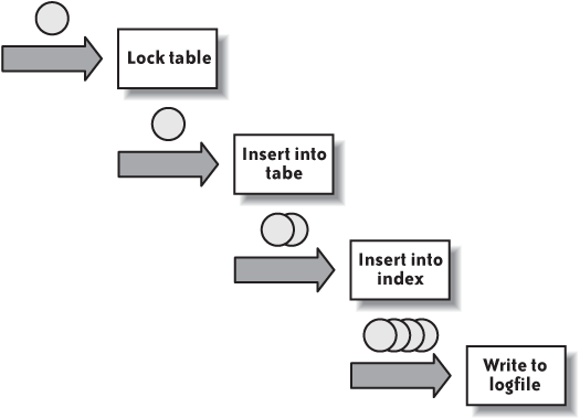
In the example where processes were removing tasks from the fifo table, I provided an example where parallelism was added to the application, and where the shared resource was the fifo table. But as I stated, the queuing model applies at many levels, from a high level to a low level. Let me drill down a little and take the simplest of examples: what happens when we insert one row into a table. As Figure 7-4 shows, we have several potential queues:
We may need to acquire a lock on the table, and if the table is already locked in an incompatible or exclusive mode, we’ll have to wait.
Then we shall either find a free slot in the table to insert data, or append a row at the end of the table. If several processes attempt to perform data insertion at the same time, while one writes bytes in memory, others will necessarily have to wait; we may also have some recursive database activity required to extend the storage allocated to the table.
Then there will probably be one or more indexes to maintain: we shall have to insert the address of the newly inserted row associated with the key value. Storage allocation work is again possible, and if several processes are trying to update indexes for the same key value, or for very close key values, they will try to write the same area of the index, and as with the table, some serialization will be required.
Then, committing the change will mean a synchronous write to a logfile. Once again, several processes cannot simultaneously write to a logfile, and we’ll have to wait for acknowledgment from the I/O subsystem to return to the program.
This list is in no way exhaustive; it is possible that some I/O operations will be needed to bring into memory pages relevant to the table or its indexes, or that foreign key constraints will have to be checked to ensure that data inserted actually matches correct values. Triggers may fire, and may execute more operations that will translate into a series of queues. Processes may also have to wait in a run queue for a processor if the machine is overloaded.
Nevertheless, the simple vision of Figure 7-4 is enough for you to understand that a single line where you spend too much time is enough to kill performance, and that when there are several places where you can wait you must be careful about not trying to optimize the wrong problem. [54] To illustrate that point I wrote and ran a simple example using a tool called Roughbench (freely available from http://www.roughsea.com and from the download area associated with this book, at http://www.oreilly.com/catalog/9780596514976). Roughbench is a simple JDBC wrapper that takes an SQL file and runs its contents repeatedly for either a fixed number of iterations or a fixed period of time. This tool can start a variable number of threads, all executing the same statement, and it can generate random data.
I therefore created the following test table:
create table concurrent_insert(id         bigint not null,
                              some_num    bigint,
                              some_string varchar(50));
In another series of runs, I made id an auto-increment column and declared it as the primary key (thus implicitly creating a unique index on it). Finally, in a last series of runs, I kept id as the primary key and partitioned the table on this column into five partitions.
I inserted rows into the table for one minute, using successively one to five threads, and checked how many rows I managed to insert.
I didn’t pick the variants of my test table at random. The indexless table is a mere baseline; in a properly designed database, I would expect every table to have some primary key or at least a unique column. But it allows us to measure the impact, both with a single thread and in a concurrent environment, of having a (nonclustered) primary key based on an auto-increment column. What I expect is, logically, lower performance with an index than without, straight from the case when I have a single thread, because index management adds up to table management. When I run more than one thread, I am interested in checking the slope of the curve as I add more processes: if the slope doesn’t change, my index adds no friction. If the slope is gentler, the index is bad for concurrency and scalability. As far as partitioning is concerned, the DBMS has to compute for each row in which partition it must go, which is done (in this case) by hashing the value of id. Partitioning should therefore make a single thread slightly less efficient than no partitioning. But I also expect processes to impede one another as concurrency increases; I have created as many partitions as my maximum number of processes with the idea of spreading concurrent inserts across the table and the index—which should not help if the whole table is locked during an insertion.
Table 7-1 shows the relative results I got committing after each insert for the MyISAM and InnoDB storage engines. [55] They don’t really match what we could have expected.
Threads | ||||||
Engine | 1 | 2 | 3 | 4 | 5 | |
No index | MyISAM | 1.00 | 1.39 | 1.45 | 1.59 | 1.50 |
Auto-increment PK | MyISAM | 0.78 | 1.19 | 1.21 | 1.36 | 1.31 |
Partitioning | MyISAM | 0.75 | 1.12 | 1.13 | 1.26 | 1.23 |
No index | InnoDB | 0.31 | 0.49 | 0.58 | 0.63 | 0.68 |
Auto-increment PK | InnoDB | 0.32 | 0.47 | 0.59 | 0.63 | 0.67 |
Partitioning | InnoDB | 0.30 | 0.46 | 0.56 | 0.61 | 0.65 |
Table 7-1 requires a few explanations:
First, scalability is very poor. Of course, multiplying by five the number of rows inserted by running five times more processes is the stuff of fairytales and marketing data sheets. But even so, as the machine was coming close to CPU saturation with five active threads, but not quite, I should have done better.
There is a very significant drop in performance with the InnoDB storage engine, which isn’t, in itself, shocking. You must remember that InnoDB implements many mechanisms that are unavailable with MyISAM, of which referential integrity isn’t the least. Engine built-in mechanisms will avoid additional statements and round trips; if the performance when inserting looks poor compared to MyISAM, some of the difference will probably be recouped elsewhere, and on the whole, the gap may be much smaller.
By the way, if you really want impressive throughput, there is the aptly named BLACKHOLE storage engine (the equivalent of the Unix /dev/null file …).
Results peak at four threads with MyISAM (on a machine with the equivalent of four processors). InnoDB starts from a much lower base, but the total number of rows inserted grows steadily, and even if scalability is far from impressive it is much better than what MyISAM displays. With InnoDB, the number of rows inserted in one minute is about 2.2 times greater with five threads than with one.
The most remarkable feature is probably that, if with MyISAM the primary key degrades performance, and if partitioning brings no improvement when concurrency increases as expected, there is no difference between the different variants with InnoDB. The uniform InnoDB performance is more striking when you plot the figures in Table 7-1 side by side as I did in Figure 7-5 (only one thing doesn’t appear clearly in Figure 7-5, which is that the ratio between best insertion rate and worst insertion rate is much better with InnoDB than with MyISAM in my test).
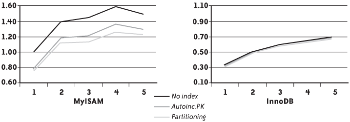
The reason the InnoDB tables show no difference is simple: the queue that blocks everything is the queue that writes to the logfile. Actually, identifying the point that slows down the whole chain would have been easier with SQL Server or Oracle than with the MySQL engine version against which I carried out my tests; in that version information_schema.global_status was rather terse on the topic of waits, and the copious output of show engine innodb status isn’t very easy to interpret when you don’t know exactly what you are looking for.
Nevertheless, the difference is obvious when I commit changes with every 5,000 rows inserted. My choice of 5,000 is arbitrary. I kept the same reference as in Table 7-1, which is the number of rows inserted in auto-commit mode into an unindexed MyISAM table.
Table 7-2 tells quite a different story from Table 7-1: with a single thread, if adding an index seems, somewhat surprisingly, to make no difference for InnoDB, partitioning still slightly degrades performance. But when you check the evolution as I added more threads, you can notice that if committing much less often has merely pushed up the MyISAM curves, removing the log bottleneck has let a new pattern emerge for InnoDB.
The difference in behavior with InnoDB appears perhaps more clearly in Figure 7-6: first, if we ignore the unrealistic case of the indexless table from three threads onward, performance with partitioning is better on InnoDB. Second, we can also check that contention is worse in the primary key index than in the table, since performance grows much more slowly with than without an index. Third, partitioning removes contention on both the table and the index and, combined with row locking, allows us to get the same insertion rate as when there is no index.
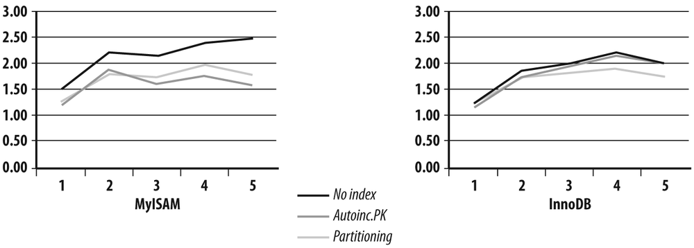
My modest machine prevented me from pushing my tests further by adding even more threads, and performance actually peaked with four threads. There are a number of lessons to learn from this simple example:
- You mustn’t start by trying to improve the wrong queue
The primary issue in the example was initially the commit rate. With a commit after each insert, it was pointless to partition the table to improve performance. Remember that partitioning a table that already contains tens of millions of rows is an operation that requires planning and time, and it isn’t totally devoid of risk. If you wrongly identify the main bottleneck, you may mobilize the energies of many people for nothing and feed expectations that will be disappointed—even if the new physical structure can be a good choice under the right circumstances.
- Bottlenecks shift
Depending on concurrency, indexing, commit rate, volume of data, and other factors, the queue where arrival rate and service time are going to collide isn’t always the same one. Ideally, you should try to anticipate; building on past experience is probably the best way to do this.
- Removing bottlenecks is an iterative process
Whenever you improve a point of friction, a queue where lines are lengthening, you more quickly release a number of requesters that are going to move to the next queue, thereby increasing the arrival rate for this next queue and possibly making it unsustainable for the service provider. You mustn’t be surprised if one performance improvement suddenly brings to light a new problem that was previously hiding in the shadow of the problem you just solved.
- You must pay attention to raw performance, but also to scalability
Raw performance and scalability aren’t always exactly the same, and it can make sense to settle for a solution that isn’t the most efficient today, but which will ensure a smooth and more predictable growth path. This is particularly true if, say, some hardware upgrade has already been scheduled for the next quarter or the quarter after the next, and you want to get as much benefit as possible from the upgrade. It may be efficient storage, or more processors, or faster processors—an improvement that may unlock one bottleneck and bring no benefit to others. Therefore, you have to juggle with the improvement paths that you have identified and choose the one that is likely to bear the most fruit.
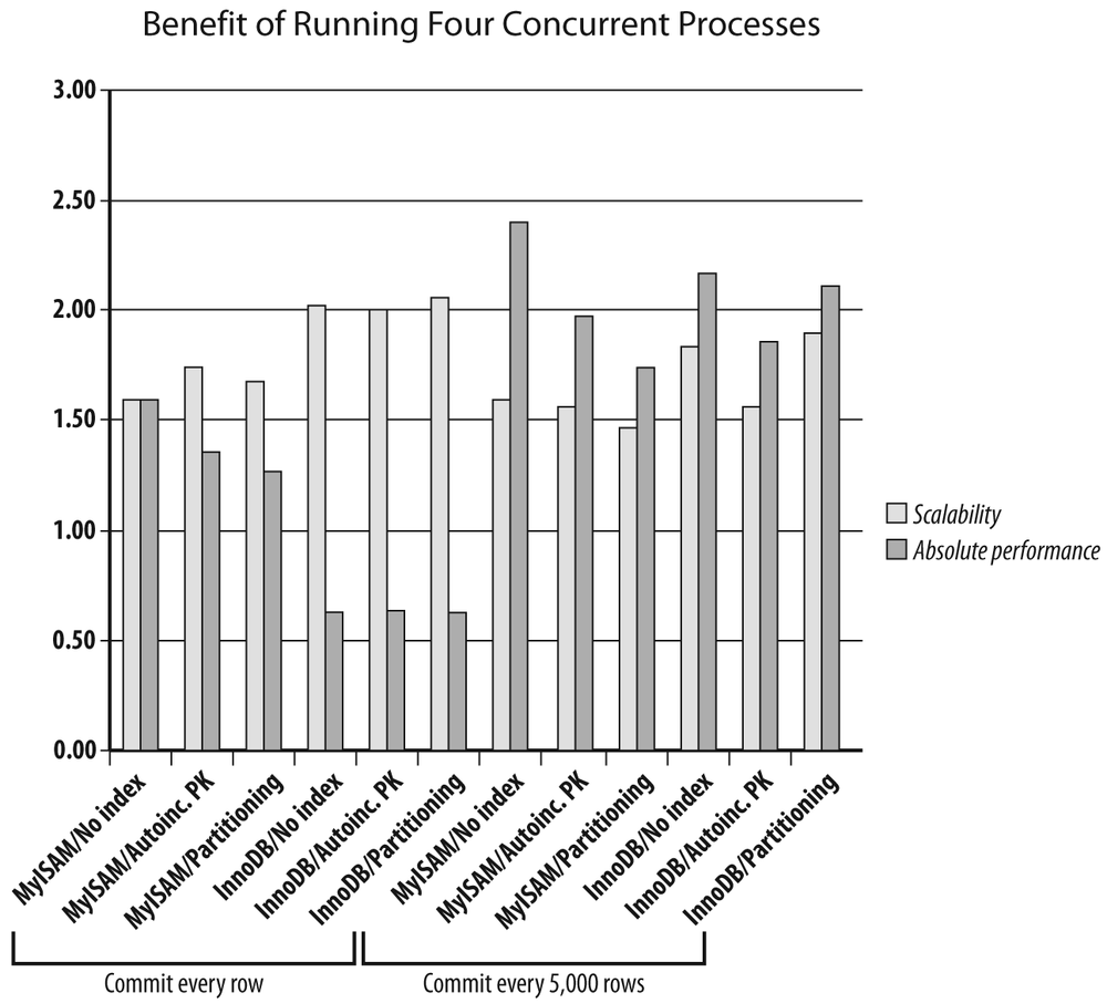
To underline the fact that raw performance under one set of circumstances and scalability aren’t exactly the same thing, consider Figure 7-7, where I charted side by side both the performance measure I got with four threads in the various configurations, as well as the ratio in performance I got by going from one thread to four (this ratio is indicated as “Scalability” in the figure). In this very limited example, you can see that the combination of partitioning with the InnoDB engine combines good performance (the best performance when you consider only the cases where a primary key is defined) and decent scalability. If you expect long-term growth, it looks like the best bet in this example. On the other hand, if the only variation in load that you expect is a sudden burst from time to time, opting for the simple MyISAM solution isn’t necessarily bad. But MyISAM plus partitioning is a solution that, once again in this example, does more harm than good (I say “in this example” because you may have concerns other than alleviating contention to use a partitioned table; simplifying archival and purges is a good reason that has nothing to do with contention and locks).
Parallelizing Your Program and the DBMS
Multiplying requesters and service providers, and trying to make everything work in harmony by minimizing locking and contention while ensuring data consistency, are techniques that aren’t always perfectly mastered but at least come easily to mind. I have much more rarely seen (outside of transaction monitors, perhaps) people trying to parallelize their program and the activity of the DBMS. Although even a modest machine can nowadays process several tasks in a truly parallel fashion, we are still using programming languages that can trace their ancestry back to FORTRAN, COBOL, and the time when a single processor was sequentially executing instructions one by one. Add to this the fact that multitasking isn’t natural to mankind (to me, at least), and it is no surprise to discover that processes are often designed to be very linear in nature.
When you execute select statements within a program, the sequence of operations is always the same, regardless of the DBMS and the language that calls it:
You get a handler to execute a statement.
You execute a call to parse the statement.
Optionally, you attach (“bind”) some input parameters to your statement.
You define memory areas where you want to retrieve the data returned from the database.
You execute the query.
As long as the return code indicates success, you fetch rows.
Sometimes some kind of compound API bundles several of the steps I just described into a single function call. But even if you ultimately get an array of values, all the steps are here.
What most people fail to realize is that almost all database calls are synchronous—that is, whenever you execute a database call, your program is idle until the call returns. This is a nonissue in a transactional environment with heavy concurrency because unless all concurrent processes are stuck on the database side in a waiting line, while your session is idle another session will put the CPU to good use. However, in some environments you can increase throughput by putting the client side to work while the DBMS is working too. A good case in point is the loading of data warehouses, a batch operation that is often known as an ETL process for Extract/Transform/Load. If, as is often the case, you extract from one database to load into another one, your program will wait twice: when you fetch the data and when you insert it.
If the DBMS API functions allow it (which isn’t always the case), you can sometimes significantly improve throughput, particularly if your transformation process needs some CPU time, by proceeding as follows (and as shown in Figure 7-8):
The extraction phase returns the first batch of data from the source database. Meanwhile, you cannot do much.
Instead of sequentially processing data and then inserting it into the target database, you copy the data just received as is to another area in memory, or you bind another area of your memory to your
selectstatement before fetching the next batch.While the second batch is fetched, another thread transforms what batch #1 returned and writes it to a third memory area. When done, it waits for extraction #2 to complete.
At the same time, a third thread takes the transformed set in the third buffer, copies it to a fourth buffer, and loads the contents of this fourth buffer into the target database.
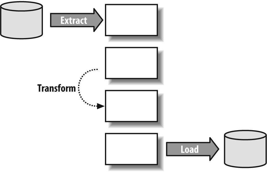
In cruise mode, you have three threads working in parallel, one fetching the nth batch of data while the second one transforms batch n – 1 and the third one loads batch n – 2.
Needless to say, synchronization may be tricky because no thread must overwrite a memory area that hasn’t yet been fully processed by the next thread in line, nor must it start to read its input if the previous thread isn’t done yet. I wouldn’t advise getting into this type of mechanism, if you don’t have a mastery of semaphores and multithreading.
You can apply the same idea to the context of applications that have to run over a wide area network (WAN). I have seen a number of applications that were accessing databases located on another continent. As long as the speed of light doesn’t get upgraded, there isn’t much you can do to avoid about 500 milliseconds of network latency between New York and Hong Kong, so using a memory cache for locally storing read-only data makes sense. Usually, what hurts is loading the cache, which is done either when you start (or restart) an application server, or when you connect if the cache is private to a session. A computer can perform a lot during a half second of network latency. If, instead of fetching data, populating the cache, fetching the next batch of data, populating the cache, and so on, you have one thread that populates the cache, allocates memory, and links data structures while another thread fetches the remaining data, you can sometimes significantly improve startup or connection times.
Shaking Foundations
In this chapter, I have shown that sometimes table partitioning is an efficient way to limit contention when several concurrent processes are hitting the database. I don’t know to what extent modifying the physical design of the database really belongs to refactoring, but because the underlying layout can have a significant impact on performance, I will now present a number of changes to consider, and explain briefly when and why they could be beneficial. Unfortunately, physical changes are rarely a boon to all operations, which makes it difficult to recommend a particular solution without a profusion of small-print warnings. You must thoroughly test the changes you want to bring, establish some kind of profit and loss statement, and weigh each increase and decrease in performance against its importance to the business. As I stated earlier, partitioning a big table that hasn’t been partitioned from the start can be a mighty undertaking that, as with any mighty undertaking, involves operational hazards. I have never seen physical design changes being contemplated for small databases. Reorganizing a big database is a highly disruptive operation that requires weeks of careful planning, impeccable organization, and faultless execution (I could add that nobody will appreciate the effort if it works as it should, but that you are sure to gain unwanted notoriety if it doesn’t); don’t be surprised if your database administrators exhibit some lack of enthusiasm for the idea. You must therefore be positively certain that the changes are a real solution, rather than a displacement of problems.
Partitioning is only one, and possibly the most commendable, of several types of physical changes you can make to a table. You can also contemplate changes that affect both the logical and the physical structure of the database—changes that may be as simple as adding a column to a table to favor a particular process, more difficult like changing the data type, or as complex as restructuring tables or displacing some part of the data to a distant database.
Altering the physical structure of the database in view of performance improvement is an approach that is immensely popular with some people (but not database administrators) who see physical reorganization as a way to give a boost to applications without having to question too many implementation choices in these applications.
It must be clear in your mind that physical reorganization of any kind is not magic, and that gains will rarely be on the same order of magnitude as gains obtained by modifying database accesses, as you saw in Chapters Chapter 5 and Chapter 6. Any alteration to the database demands solid reasons:
If you poorly identify the reason for slowness, you may waste a lot of effort. The previous example with the concurrent insertions is a case in point: with a
commitafter each insert, partitioning brought no measurable benefit because the bottleneck was contention when writing to the journal file, not contention when writing to the table or to the primary key index. Only after having solved the logfile issue does the bottleneck shift to competing insertions into the table and (mostly) the index, and does partitioning help to improve performance.Another important point is that the benefits you can gain from physical reorganization usually stem from two opposite ends of the spectrum: either you try to cluster data so as to find all the data you need when you request it in a few pages, minimizing the amount of memory you have to scan as well as the number of I/O operations, or you try to disseminate data so as to decrease contention and direct various “requesters” to different “queues.” It is likely that any partitioning will adversely affect some parts of the code. If you improve a critical section and worsen an ancillary part, that’s fine. If you replace a problem with another problem, it may not be worth the trouble.
With that being said, let’s now see how we can speed up processing.
Marshaling Rows
As we just saw, partitioning is the best way to decrease contention, by making concurrent processes hit different physical areas of a single logical table. But another reorganization that matters is to do whatever is needed to cluster together rows that usually belong to the same result set. Such an organization is more important for rows that are retrieved through a range scan on an index—that is, a condition such as the following:
and some_indexed_column between<min value>and<max value>
I mentioned in Chapter 2 the relationship between the order of the keys in the index and the order of the corresponding rows; nowhere does this relationship matter as much as in a range scan. In the worst case, what can happen is something that looks like Figure 7-9: when you scan your index, the successive keys that you meet all refer to rows that are stored in different pages of the table. [56] Such a query is likely to result in many I/O operations because only some of the pages will already be in memory when they’re needed.
To this you can add CPU waste because each page will need to be accessed in memory to retrieve only one row.
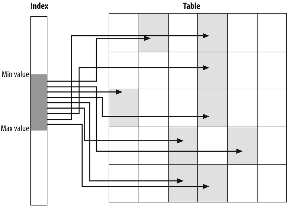
Of course, the ideal case would be to find all the rows addressed by the set of keys gathered in a single page, or in as few pages as possible: this would minimize I/O operations, and scanning the pages would really be profitable. If we want such an ideal situation for all possible ranges of keys, we have only one solution: we must find the rows in the table in the same order as the keys in the index. To achieve this goal, either we re-create the table and reinsert the rows after sorting by the index key (with the risk of having to perform the same operation at regular intervals if rows are regularly inserted, updated, and deleted), or we define the table to have a self-organizing structure that suits our needs. We can reach our goal by defining the index as a clustering index with SQL Server or MySQL and the InnoDB engine, or defining the table as an index-organized table (the Oracle equivalent). [57]
We must be aware of a number of conditions:
Rows are ordered with respect to index
idx1or with respect to indexidx2, but not with respect to both, unless there is a very strong relationship between the column(s) indexed byidx1and the column(s) indexed byidx2—for instance, an auto-incrementing sequence number and an insertion date. One index, and therefore one category of range searches, will be unfairly favored over all others.The index that structures the table usually has to be the primary key index. It may happen that, if the primary key is made of several columns, the order of the columns in the primary key won’t quite match the order we want. That would mean we must redefine the primary key, which in turns means we must redefine all foreign keys that point to that primary key, and perhaps some indexes as well—all things that can take you pretty far.
Insertions will be costlier, because instead of carelessly appending a new row, you will have to insert it at the right place. No, you don’t want to update a primary key, and therefore, updates aren’t an issue.
Tables that are wide (i.e., have many columns) make insertions much more painful and such an organization doesn’t benefit them much: if rows are very long, very few rows will fit into one page anyway, and their being suitably ordered will not make much of a difference.
Contention will really be severe if we have concurrent inserts.
When some of these conditions cannot be satisfied, partitioning once again can come to the rescue. If you partition by range over the key, data will not be as strictly ordered as in the previous case, but it will be somewhat herded: you will be sure that your entire result set will be contained in the partition that contains the minimum value and all the following partitions, up to the partition that contains the maximum value for your scan. Depending on the various conditions provided in the query, it is even possible that an index will not be necessary and that directly scanning the relevant partitions will be enough.
As with clustering indexes, this will be a use of partitions that may increase rather than decrease contention. The typical case is a date partitioning by week on the row creation date in a table that keeps one year of data online: at any given moment, the most active part of the table will be the partition that corresponds to the current week, where everyone will want to insert at once. If data insertion is a heavily concurrent process, you must carefully choose between using partitioning that spreads data all over the place, and partitioning that clusters data. Or you can try to have your cake and eat it too by using subpartitioning: suppose the table contains purchase orders. You can partition by range of ordering dates, and within each partition divide again on, say, the customer identifier. Concurrent processes that insert purchase orders will indeed hit the same partition, but because presumably each process will deal with a different customer, they will hit different subpartitions if the customer identifiers don’t hash to the same value.
Subpartitioning (which I have rarely seen used) can be a good way to keep a delicate balance between conflicting goals. With that said, it will not help you much if you run many queries where you want to retrieve all the orders from one customer over the course of a year, because then these orders will be spread over 52 subpartitions. I hope you see my point: partitioning and subpartitioning are great solutions for organizing your data, but you must really exhaustively study all the implications to ensure that the overall benefit is worth the trouble. In a refactoring environment, you will not be given a second chance, and you really need to muster the support of all people involved—database administrators in particular. Whenever I encounter a table with more than one million rows, partitioning automatically appears on my checklist with a question mark. But whether I recommend the partitioning always depends. I’m usually very suspicious when I encounter a table that contains several hundred millions of rows and isn’t partitioned; however, some tables in the range of one million to tens of millions of rows are sometimes better left unpartitioned.
Splitting Tables
Whether you use a clustering index, turn your table into an index-organized table, or slice and dice it into partitions and subpartitions, you “merely” affect the physical structure of the database. For your programs, the table will remain the same, and even if the reorganization that you decide upon will make you hated intensely by several people who would have rather spent their weekend doing something else, you can at least pretend that it will be transparent for programs (if you remember Chapter 5, you may nevertheless have to review a few queries). Some other physical alterations to the database may bring significant benefits, but require (slight) adjustments to queries.
A frequent case for poor performance is the existence of tables with very wide rows, for a reason similar to the example shown in Figure 7-9: index range scans hit mostly different blocks. In that case, the cause isn’t row ordering, and reorganizing the table as we saw previously will not help. The cause is that because rows are wide, each page or block stores very few rows. This situation frequently occurs when a table contains multiple long varchar columns, text columns, [58] or large objects (LOBs)—especially when they are updated often, causing fragmentation in the data blocks. When LOBs are very big, they are stored in special pages, and rows contain only a pointer to these pages (the pointer is sometimes known as the locator). But because the use of indirections can severely impact performance, smaller LOBs are often stored in-row (up to 4,000 bytes with Oracle and 8,000 bytes with SQL Server; with MySQL it depends on the storage engine). You don’t need many 2,000- or 4,000-character columns in a row to be filled to have a very low density of rows per table page and ruin range scans.
One solution may be to split a wide table t into two tables, as I show in Figure 7-10 (the circles represent the primary key columns). The case is based on the fact that long columns rarely participate in queries that return many rows, and that joins and extra fetches add a negligible overhead to small result sets. In such a case, you can try to isolate into a table that I have renamed t_head, which contains all (narrow) columns that are indexed, plus a few other columns that may be critical when identifying result sets. As a result of the column selection, rows in t_head are short, density is high, and we can even use a clustering index or partition the table and ensure that index range scans (or full table scans, for that matter) will hit a small number of pages, full of information.
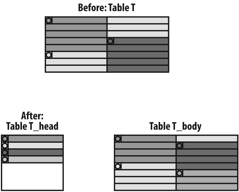
All the long columns, plus the primary key columns that are duplicated, are moved to a second table called t_body. This second table behaves as a kind of secondary storage, “indexed” by the same primary key as t_head.
In such a case, because the initial table disappears, a number of changes must be brought to the programs:
All
selectand someupdatestatements that hit only columns that now belong tot_headort_bodymust reference the new table to take advantage of the new structure. Forupdatestatements it may be tricky. It depends on how the table is initially populated. It may happen that when you insert a new row you set values only for columns that now belong tot_head. In that case, there is no reason to insert intot_bodya matching row that is empty except for the primary key columns. But then, the very firstupdateapplied to a column oft_bodymust translate to aninsertstatement—by catching an exception, not by checking beforehand whether the row exists!All
selectstatements that refer to columns now split betweent_headandt_bodymust refer to a view that joinst_headtot_bodyso as to look like the original table. The join may need to be an outer join, becauset_bodymay not yet contain a matching row for each row int_head.As previously explained,
insertstatements intotmay become either successive inserts intot_headandt_body, or inserts intot_headfollowed much later by inserts intot_body.For
deletestatements, the case is simpler: you merely have to delete from the two tables in a single transaction.
Altering Columns
You can make several changes to columns: you can play on their contents, split them, or add new columns. Like all physical changes, none of these changes is to be undertaken lightly, and because the logical structure of the tables is modified there must be parallel changes in the programs.
Changing the contents
One particularly effective change that you can experiment with, even if it looks pretty insignificant, is to play on the null/not null attribute of a column. As a general rule, any column that always contains data should be declared as not null (null is the default with Oracle). It can make a significant difference for the optimizer to know that there is always a defined value in the column, because it affects join strategies as well as subqueries and cardinality estimates. Even when the column may not be populated, it can make sense to use a default value. If you have an index on a single column that can contain null values, a product such as Oracle doesn’t index null values, and a condition such as the following will necessarily translate (if there is no other condition) into a full scan, even if the majority of rows contain values:
and column_name is null
Using a default value would allow a straight and efficient index search. [59]
An opposite strategy is sometimes successful: if a column contains nothing more than a Y/N flag and the only rows you are interested in are the ones for which the value is Y (a minority), replacing a value that isn’t much loaded with significance, such as N, with null may make indexes and rows more compact (some products don’t store nulls) and searches slightly more efficient (because there are fewer blocks to read). But in most cases, the difference will be so modest that it will not really be worth the effort; besides, some database engines now implement compression mechanisms that render this optimization moot.
Splitting columns
Many performance issues stem directly from the lack of normalization of databases—particularly not abiding by first normal form, which states that columns contain atomic values with regard to searches, and that conditions should apply to a full column, not to a substring or to any similar subdivision of a column. Of course, partial attempts at normalization smack of despair: too often, proper normalization would mean a total overhaul of the database design. Such a grand redesign may be badly necessary, but it is likely to be a hard sell to the powers that hold the purse. Unfortunately, half-baked attempts at fixing glaring inadequacies don’t often make a bad situation much better. Suppose you have a column called name which contains first names, middle initials, and last names. This type of column turns even simple searches into operations from hell. Forget about sorts by family name (and if the family name comes first, you may be sure to find in the list some names of foreign origin for which the first name will have been mistaken for the family name), and searches are likely to end up in pathetic conditions for which indexes are utterly useless, such as the following:
where upper(name) like '%DOE%'
In such a case, it doesn’t take long to realize that the column content should be split into manageable, atomic pieces of information, and perhaps that forcing data to uppercase or lowercase on input might be a good idea, even if the rendition means new transformations. But the question, then, is whether information should be duplicated, with the old column kept as is to minimize disturbances to existing programs, or whether you should be more radical and get rid of it after its replacement. The big issue with keeping the old column is data maintenance. If you don’t want to modify the existing insert statements, either you populate the new columns through a trigger or you define them (with SQL Server) as persisted computed columns that you can index. Whether you call the function that chops the string from within a trigger or in the definition of the computed column doesn’t make much of a difference. The function call will make inserts and updates (relatively) slow, and automated normalization of strings is likely to be very bug-prone as long as names don’t follow very simple patterns. As a result, you’ll probably end up spending much more time trying to fix the transmogrifying function than modifying the insert and update statements in the first place. It may not look so initially, but it may be safer to take the jump, burn your vessels, and not try to maintain a “compatibility mode” with what you reckon to be a poor choice of implementation.
Adding columns
The opposite of trying to normalize data is the more popular course of action, which is to denormalize it. Most often, the rationale behind denormalization is either the avoidance of joins (by propagating, through a series of tables, keys that allow shortcuts), or the avoidance of aggregates by computing values for reporting purposes on the fly. For instance, you can add to an orders table an order_amount column, which will be updated with the amount of each row referring to the order in the order_details table, where all articles pertaining to the order are listed one by one.
Denormalization poses a threat to data integrity. Sooner or later, keys that are repeated to avoid joins usually land you in a quagmire, because referential integrity becomes nearly impossible to maintain, and you end up with rows that you are unable to relate to anything. Computations made on the fly are safer, but there is the question of maintenance: keeping an aggregate up-to-date throughout inserts, updates, and deletes isn’t easy and errors in aggregates are more difficult to debug than elsewhere. Moreover, if the case was sometimes rather good for this type of denormalization in the early days of SQL databases, extensions such as the addition of the over () clause to the standard aggregate functions make it much less useful.
The most convincing uses I have seen for denormalization of late were actually linked to partitioning: some redundant column was maintained in big tables where it was used as a partition key. This represented an interesting cross between two techniques to make data storage more suitable to existing queries.
Very often, denormalization denotes an attempt at overlaying two normalized schemas. Normalization, and in particular the very idea of data atomicity that underlies the first normal form, is relative to the use we have for data. Just consider the case when, for performance reasons, you want to store aggregates alongside details. If you were interested in details and aggregates, there would be no reason to maintain the aggregates: you could compute them at almost no extra cost when retrieving the details. If you want to store the aggregates, it is because you have identified a full class of queries where only the aggregates matter; in other words, a class of queries where the atom is the aggregate. This isn’t always true (e.g., a precomputed aggregate may prove handy in replacing a having clause that would be very heavy to compute on the fly), but in many cases denormalization is a symptom of a collision between operational and reporting requirements. It is often better to acknowledge it, and even if a dedicated decision support database [60] is overkill, to create a dedicated schema based on materialized views rather than painfully maintaining denormalized columns in a transactional database.
Materializing views
Materialized views are, at their core, nothing more than data replication: usually, a view stores the text of a query, which is reexecuted each time the view is queried. The creation of a materialized view is, in practice, equivalent to the following:
create table materialized_view_name
as
select ....
With SQL Server, a view is materialized when you create a unique clustered index on it. Afterward, all modifications to base tables are propagated to the copy. With Oracle, there is a special create materialized view statement, in which you specify, among other things, how the view must be refreshed: automatically each time a transaction on the base tables commits, or asynchronously through a “refresh” job that is scheduled by the DBMS. In this latter case, the materialized view can be either completely refreshed (a kind of cancel and replace mode) or incrementally refreshed, which requires the creation of log tables associated to the base tables. A refresh that occurs when a transaction commits requires a log. MySQL up to and including version 6.0 doesn’t support materialized views, but mechanisms such as those implemented by Oracle can be developed with triggers (the triggers that Oracle uses to manage materialized views have been incorporated into the kernel in Oracle 8i, but previous releases were using regular triggers); you can automatically generate these triggers by querying the information_schema views.
Everything has a price, and the existence of a materialized view means that all operations that change the base tables will cost more and take longer, because of the operations needed to record and to apply the changes to the materialized view on commit—unless you have opted for a full refresh, which could be a viable solution if there may be some lag between data in the materialized view and data in the base tables, and if refreshes are part of nightly batch processes.
There are basically two uses for materialized views:
The first use, which I just suggested, is as a kind of light ETL process. If the overhead on the base tables is bearable—and if you manage to isolate a part of your application that is more about reporting or decision support—materialized views, which can be indexed so as to get the best performance, will be your powerful allies. Oracle and SQL Server are even able to recognize the query that was used to create the materialized view, and hit the prebuilt result set rather than execute the query when they encounter it.
The second use is when one or several of your queries refer to distant tables on another server. If you do not need a synchronous vision of data, getting a local copy will give the optimizer more freedom to choose a good path. When you hit a distant table, nested loops usually aren’t an option, because each iteration would require a round trip over the network. Very often, the SQL engine will lap up the data over the network, store it locally (unindexed), and do its best to run the query. By using a materialized view, you can have your local copy, you can index it as you want, and you can have nested loops if they happen to be the most efficient way to run the query.
Much too often, developers consider materialized views as a panacea. I once attended a meeting with a handful of seasoned DBAs where some developers suggested creating, for multidimensional analysis, 13 materialized views on a table that was to store around one billion rows. The DBAs almost fainted. More recently, I saw a developer using materialized views to solve performance issues with queries that were referring to the most recent date in a table destined to hold two years’ worth of data. It contained a series of materialized views that followed this pattern:
select *
from t
where date_column = (select max(date_column) from t)
On closer inspection, the (big) tables weren’t partitioned, and the only indexes were primary key indexes—on surrogate keys.
As I hope this book has demonstrated, creating materialized views, in spite of their undeniable usefulness in some cases, isn’t the first step to take when trying to improve performance.
[47] Which is likely to wreak havoc.
[48] True story. It was cleverly improved in the next version of the program, which fixed some severe performance issues: not by adding a where clause (stop dreaming), but by using a local cache on the user’s PC.
[49] Merge joins are very close in spirit to hash joins.
[50] Note that it is possible with Oracle and some interfaces to execute an update and return a value at once.
[51] Oracle never blocks other readers.
[52] Although Oracle allows you to specify that the lock command should return an error, if it cannot be satisfied immediately.
[53] I am not a great fan of temporary tables. But, as with all features, they have their use.
[54] I cannot do better on this topic than redirect Oracle users to Optimizing Oracle Performance by Cary Millsap with Jeff Holt (O’Reilly), which explains in detail how to identify where time is really spent and the various traps to avoid. A chapter of the book is also dedicated to queuing theory for database practitioners.
[55] Because results obtained on my relatively modest dual-core biprocessor test machine have little universal value, I have expressed all results in relation to the number of rows I managed to insert with one thread into the unindexed MyISAM table. For the record, it was about 1,500 rows per second.
[56] That’s blocks for you Oracle folks.
[57] There are other possibilities, such as adding more columns to the index so as to find all the information in the index, which avoids the indirect access to the table.
[58] Clob columns in Oracle.
[59] With dates, and, as a general rule, all columns on which range searches are performed, dummy values that replace null columns may give the optimizer the wrong idea about the scope of values, and therefore the wrong idea about what percentage of a table a range scan is going to sweep through.
[60] Which might use a different technology, such as an OLAP cube, or column-based processing such as Sybase’s IQ product.