13

The Option Value of Uncertain Projects

Up to now in this book, an investment project was described by its flow of costs and benefits. When we introduced uncertain cash flows in the previous chapter, we did not allow the decision maker to react to the potential new information that could arise about the profitability of the project. The only decision was whether or not to invest in the project. This is quite counterintuitive. Indeed, the most basic idea of risk management is that flexibility is crucial to behaving efficiently in an uncertain world. According to this idea, an investment project is not univocally characterized by its cash flow. Rather, it is described by an oft complex and intricate dynamic decision process, where decisions must be made at different points in time. When a country decides to invest in a civil nuclear program, it must first decide to start the program, with a research and development phase that is followed by the decision to build a first prototype electricity plant. If it is successful, the decision must be made to implement the construction of several power plants in the country. Afterward, the country has the option to expand the program, or to use the accumulated experience to start a second-generation program. Similarly, when one considers the possibility of creating a high-speed railway between New York and Philadelphia, one should include in the evaluation of this investment project the option value that this first investment generates to extend the line to Boston, or to Washington. When initiating a program of abatement of greenhouse gases, one can start with a slow reduction rate with the idea that one will have the option to strengthen the program in the future if the economic and technological environment becomes more favorable.

If no new information is made available between different decision dates, the standard NPV approach remains valid to evaluate this kind of project. One just needs to make sure that all components of the project with a positive incremental NPV are included in the project from the beginning. But in most applications, new information is revealed over time about variables that may affect the profitability of the investment project and its extensions. During the implementation phase of the nuclear program, one can get new information about costs and safety, about the competitiveness of alternative technologies to produce electricity, or about the evolution of the demand for electricity. A similar observation can be made for the illustration about the high-speed train. Concerning the climate change application, the U.S. government has often justified its low-key position to fight climate change on the basis that it is better to wait for better information about the intensity of the problem, and about the cost of green technologies. Thus, the full characterization of an investment project can be an intricate combination of decisions and information revelations scattered along the time line. In some circumstances, the flow of information depends upon past decisions (such as R&D and experimentation).

In this context, the standard NPV approach is not adapted, since the cash flows to be discounted depend upon decisions to be made in the future that themselves depend upon information not yet available today. The method to be used in this context is based on backward induction, in which the standard NPV is used in each decision date, starting from the last one, and contingent to each possible signal observable at that date. In each decision date but the last one, the information-dependent optimal choices that will be made in the future are used to compute the risk-adjusted NPV that drives the decision at that date. By construction, these net present values include a positive option value coming from the possibility to flexibly react to future information. These observations were first made independently by Henry (1974) and Arrow and Fisher (1974). Since then, an important literature on option value has been developed, which is nicely summarized by Dixit and Pindyck (1994).

In the remainder of this chapter, I first illustrate the notion of an option value with a simple numerical example. I then examine a more sophisticated application with a Poisson two-armed bandit. In the first case, there is an option value to wait. In the second case, there is an option value to experiment. Applications are very wide in spectrum, from finance to climate change through corporate governance, R&D strategy, public health policy, or the extraction of natural resources.

A SIMPLE NUMERICAL EXAMPLE

Consider a simple investment project. For the next ten years, it yields a sure annual payoff that is normalized to unity. The annual payoff beyond this time horizon is uncertain. With equal probabilities, it will be either 1.6 forever or 0.4 forever. We assume that these events are not correlated to other macroeconomic variables, as economic growth. There is an irreversible sunk cost to implement the project which is equal to 20, independent of the date at which the project is implemented. We assume that the risk-free discount rate is 4%, and is constant over time. Should one invest in this project? Because the project is small and uncorrelated with aggregate growth, risk neutrality can be assumed.

Because the annual payoffs are independent with respect to the growth of aggregate consumption, the beta of the project is zero, and one can use the risk-free rate to discount the expected cash flows. If one invests today, one gets

Because the expected net present value of the strategy to invest today is positive, this suggests that investing today is optimal. If the project is financed by a perpetuity, the investor will have to pay an annual interest of 0.8. The net cash flow of the project is thus equal to 0.2 over the first ten years. It is afterward equal to 0.8 in the good state of nature, or –0.4 in the bad state of nature. In that state of nature, the investor will feel regret about the initial decision to invest.

This strategy would indeed be optimal if investing today or never investing were the only two options. In reality, the right question today is whether to invest today, or to postpone that decision to the future. As is often the case in investment decisions, the problem is dynamic in nature, because the decision to invest can be postponed to get more information. Of course, postponing the investment decision by one year has no interest. It would save one year of interest payment on the perpetuity associated with the financing of the investment cost, but the investor would give up the first annual cash flow. The net benefit of this equals 20 × 0.04 – 1 = –0.02, which is negative. Waiting to invest has a cost expressed by the difference between the unearned annual cash flows and the saved cost of capital.

The only benefit to postponing the decision would be to learn the state of nature about the long-term profitability of the project, and this would require waiting ten years. If one does this, one must separately consider the two alternative scenarios. In the bad state of nature, it is obvious that not investing is optimal, because the value of the perpetuity of 0.4 is not enough to compensate for the sunk cost (10 < 20). In the good state of nature, it is optimal to invest in the project for the symmetric argument. Evaluated at that time and in that state of nature, the NPV of investing in the project equals (1.6/0.04) – 20 = 20, which is positive. One is now confronted with two alternative strategies. The first strategy consists of investing today, with an expected NPV of 5. The second strategy consists of investing in ten years only in the good state of nature. In short, it yields a single cash flow of 20 with probability 50% in ten years. Evaluated from today, the expected present value of this alternative project equals 0.5 × 20 × e^-0.04×10 = 6.7. This is larger than the expected NPV from investing today. In spite of the fact that investing today has a positive expected NPV, postponing the decision to invest in ten years is optimal. The value of information obtained from waiting is larger than the cost to wait coming from giving up ten years of positive cash flows net of the cost of capital.

The literature on real option values relies heavily on this methodology based on backward induction. When there exist traded assets whose prices are correlated with the payoff of the project, the option value can be evaluated by using techniques of pricing by arbitrage, as in the financial literature on options initiated by Black and Scholes (1973). McDonald and Siegel (1986) evaluate by arbitrage the option value to wait in the context of a cash flow governed by a geometric Brownian motion. Describing the resolution of the decision problem in this context would require using more sophisticated methods based on the Ito’s Lemma, which is beyond the scope of this book.

LEARNING IN THE POISSON BANDIT PROBLEM

In this section, we consider a more sophisticated investment problem with two mutually exclusive projects. In order to obtain an analytical solution to this problem, we depart from the standard discrete time approach used in this book to consider a continuous time framework. The first project is safe and yields a constant cash flow _s. Its NPV equals

The other project is uncertain. It entails payoffs at random dates in the future, with an uncertain frequency. More specifically, the uncertain project distributes a lump-sum payoff h at random dates according to a Poisson process with parameter λ. This means that, when dt is small, there is a probability λdt to get a cash flow h in any time interval [t, t + dt]. The problem is that parameter λ is unknown. It can take two possible values, λ₀ and λ₁ ≥ λ₀. At any date t, the beliefs of the decision maker are summarized by the probability p_t that the true value of λ is the good one λ₁. The expected Poisson parameter at date t is thus λ(p_t) with

Suppose that the subjective belief at date 0 about facing a good project with λ = λ₁ is p₀. Suppose also that the decision maker is risk-neutral, for example because the uncertain project is fully diversifiable.

Consider first a rigid context in which the take-it-or-leave-it decision to invest must be made at date 0, and is irreversible. In such a context, it is efficient to invest in the uncertain project if and only if its subjective discounted expected payoff, λ(p₀)h/r, is larger than s/r, the sure discounted payoff of the safe project, where r denotes the discount rate. This is the case if and only if the probability of facing a good investment project is larger than p^m = (s/h-λ₀)/(λ₁ –λ₀). In order to make the problem interesting, we hereafter assume that the safe project is preferred to the bad risky project (s > λ₀h), but is dominated by the good one (s > λ₁h). This implies that p^m ∈[0,1].

The evaluation problem becomes more complex if we relax the irreversibility assumption. Let us alternatively assume that the decision maker can switch from one project to the other at any time. The problem of evaluating the uncertain project and of describing the associated optimal investment strategy is referred to in the literature as the “two-armed bandit” problem, with one safe arm, and one uncertain arm. Rothschild (1974) and Bolton and Harris (1999, 2000) are the classical references cited in this field.

When the decision maker is on the safe project, he is unable to get any information about the uncertain project. In this alternative context, it may be desirable to first invest in the uncertain project even when p₀ < p^m, because of the value of learning the true value of l by doing so. In a word, it may be optimal to experiment to learn about the true value of l. If the observed frequency of Poisson events is too low, that would signal a bad project, and the agent should switch to the safe investment sooner or later. In the remainder of the chapter, we determine the option value generated by investing in the uncertain project.

We first examine the intensity of learning in an interval of time [t, t + dt], as described in figure 13.1. Suppose that p_t is the probability of facing a good project, as evaluated at date t. If no payoff is observed in this interval, the probability of facing a good project will be lowered. Otherwise, this posterior probability will be increased. In order to quantify the dynamics of beliefs, we use Bayes’ rule under the following probabilistic scenarios in the interval of time [t, t + dt]:

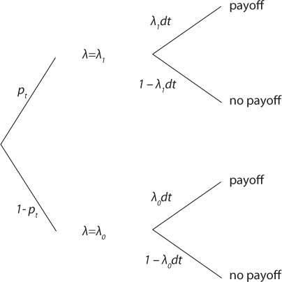
Figure 13.1. Scenarios of learning in the two-armed Poisson bandit problem.

Suppose that no payoff is observed during this interval of time. In that case, the beliefs at date t + dt must equal

It implies that when no payoff is observed, the probability to face a good project decreases smoothly at rate (1 – p_t)(λ₁ – λ₀) per unit of time. On the contrary, if a payoff is observed during the interval of time [t, t + dt], the beliefs at time t + dt must satisfy

Thus, when a payoff is obtained in [t, t + dt], the probability of a good project has an upward jump from p_t to j(p_t) = p_tλ₁/λ(p_t). The intensity of the upward jump goes to zero when p_t tends to unity. Observe that p = 1 is an absorbing state.

Of course, the stochastic process of the beliefs p_t is a martingale in the sense that Ep_t+dt = p_t. One can compute the rate of reduction in the subjective probability of facing a good project conditional to actually facing a bad project (λ = λ₀). We have that

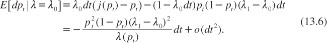
In this context, the expected value of the Poisson parameter l declines in expectation:

A symmetric result is obtained conditional to the good project.

OPTIMAL INVESTMENT STRATEGY IN THE POISSON BANDIT PROBLEM

Thus, investing in the uncertain project conveys information about its quality. Because we assume that the agent can switch to the safe project if the uncertain one has a low subjective expected return, this learning process has a value that should be taken into account in the evaluation process. Let k_t denote the strategy at date t, where k_t = 1 means that the agent invests in the uncertain project at date t, and k_t = 0 means that the agent invests in the safe project at that date. We focus on Markov strategies, that is, strategies that only depend upon current beliefs: k_t = k(p_t). We are looking for the Markov strategy that maximizes the discounted expected cash flow extracted from the investment:

where the expectation operator is over the stochastic processes of p_t and k_t.

We hereafter follow the resolution strategy proposed by Keller and Rady (2010). The Bellman equation for this problem can be written as

Because dt is small, this can be rewritten as

Indeed, if the agent does not experiment (k = 0), there is no learning and dp = 0. If she experiments, dp will be adapted according to the Bayes rule as described earlier, and U(p + dp) will differ from U(p) according to the second line of equation (13.10). After eliminating U(p) in both sides of this equality, it is rewritten as follows:

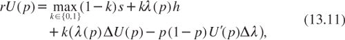
where ΔU(p) = U(j(p)) – U(p) and Δλ = λ_λ – λ₀. The objective to maximize in the right-hand side of this equation is the sum of the expected payoff and of the value of information. Conditional to the current belief p, it is optimal to experiment if

In that case, the discounted expected value of the uncertain project satisfies the following ordinary differential-difference equation:

It can be shown that the solution of this equation is

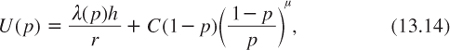
where C is a constant of integration and m is the unique positive root of the following equation:

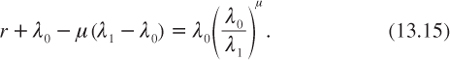
It can be shown that m is increasing in the discount rate r. Equation (13.14) shows that in the continuation region (where experimenting is optimal), the discounted expected payoff of the uncertain project equals the subjective expected value of its cash flow (λh/r) plus an option value V of switching to the safe project.

Of course, investing in the safe strategy is an absorbing state, with U(p) = s/r. Investing in the safe project is optimal if the probability of facing the good project is below a threshold p^* that is obtained jointly with the constant of integration C by solving the joint value-matching condition U(p^*) = s/r and the smooth-pasting condition U(p^*) = 0. Following Keller and Rady (2010), the solution of this system of two equations with two unknown is

and

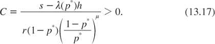
It is easy to see that the critical probability p^* is smaller than the myopic threshold p^m = (s/h − λ₀)/(λ₁ − λ₀). This expresses the fact that it may be optimal to experiment when the expected return of the uncertain project is below the sure return of the safe project.

Because C is positive, the option value V(p) to switch to the safe project is positive in the continuation region p > p^*. It takes the following form:

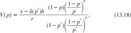
It is not surprising, then, that, at p = p^*, the option value V(p^*) = (s – λ(p^*)h)/r just compensates for the difference between the discounted expected cash flows of the two projects.

Let us illustrate the problem with the following numerical example. Suppose that the safe asset yields a constant payoff s = 1 per unit of time. The uncertain project generates a payoff h = 10 ten times larger, but only at random dates, with a frequency that equals either λ₀ = 5% or λ₁ = 15%. It yields the myopic strategy to invest in the uncertain project if the subjective probability of facing a good project is larger than p^m = 50%. Suppose also that the discount rate is r = 4%. Equation (13.15) exhibits solution m = 0.657. We also get from equation (13.16) that the critical subjective probability of the good project presented previously which it is optimal to invest in the uncertain project is p^* = 28.4%. We finally have that C = 4.1, so that in the continuation region p > p^*, the discounted expected payoff of the optimal investment strategy equals

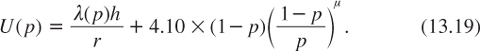
This function is depicted in figure 13.2. The option value can be quite large. For example, if the subjective belief is p = 50%, the option value is V(0.5) = 2.05, or 7.6% of the total value of the project U(0.5) = 27.05.

As seen from this analysis, option values add an important degree of complexity to the evaluation analysis. Defining an efficient dynamic risk management strategy is inescapably difficult when the current uncertainty is subject to further revision due to the arrival of new information. The citizen, the judge, the politician, and the entrepreneur may have a hard time determining this strategy. How many vaccines should one purchase against a possible epidemic of unknown severity? How much effort to abate greenhouse gases whose effects on the environment are still imperfectly known? Should we impose a moratorium on some new biotechnologies yielding genetic manipulations whose long-term ecological impacts are uncertain? The precautionary principle that emerged at the Rio conference in 1992 is aimed at providing a cautious decision principle in the context of evolving uncertainties. My interpretation of this principle is that the theory of real option values should be considered seriously for the evaluation of public policies (Gollier and Treich 2003).

Figure 13.2. The discounted expected payoff of the optimal investment strategy, with s = 1, h = 10, λ₀ = 5%, λ₁ = 15%, and r = 4%. The dashed curve is the value of the project when using the myopic strategy.

SUMMARY OF MAIN RESULTS

1.  In an uncertain world, flexibility is crucial. Irreversible decisions have a hidden cost coming from the subsequent inability to use information that will emerge in the future.

2.  The theory of real option value has the objective to adjust the standard cost-benefit methodology, which is static by nature, in order to integrate these dynamic aspects of the evaluation problem.

3.  The computation of option values must be done by backward induction. At each node of the decision tree, the optimal decision is made by taking into account the optimal decisions in the subsequent nodes of that part of the tree.

4.  In the case of the two-armed Poisson bandit problem, an optimal stopping-time strategy can be analytically derived. It is optimal to experiment with the uncertain project as long as the continuously updated probability of facing a good project is large enough. The computation of the minimum probability and of the associated NPV of the uncertain project takes into account an option value of learning.

REFERENCES

Arrow, K. J., and A. C. Fisher (1974), Environmental preservation, uncertainty and irreversibility, Quarterly Journal of Economics, 88, 312–319.

Black, F., and M. Scholes (1973), The pricing of options and corporate liabilities, Journal of Political Economy, 81 (3), 637–654.

Bolton, P., and C. Harris (1999), Strategic experimentation, Econometrica, 67, 349–374.

Bolton, P., and C. Harris (2000), Strategic experimentation: the undiscounted case, in P. J. Hammond and G. D. Myles (eds.), Incentives, Organizations and Public Economics—Papers in Honour of Sir James Mirrlees, Oxford: Oxford University Press.

Dixit, A. K., and R. S. Pindyck (1994), Investment under Uncertainty, Princeton: Princeton University Press.

Gollier, C., and N. Treich (2003), Decision-making under scientific uncertainty: The economics of the Precautionary Principle, Journal of Risk and Uncertainty, 27, 77–103.

Henry, C. (1974), Investment decisions under uncertainty: the irreversibility effect, American Economic Review, 64, 1006–1012.

Keller, G., and S. Rady (2010), Strategic experimentation with Poisson bandits, Theoretical Economics, 5(2), 275–311.

McDonald, R., and D. Siegel,(1986), The value of waiting to invest, Quarterly Journal of Economics, 101, 707–728.

Rothschild, M. (1974), A two-armed bandit theory of market pricing, Journal of Economic Theory, 9, 185–202.