4

Random Walk and Mean-Reversion

The first part of this book concluded that there is a solid scientific basis to recommend the use of a discount rate around 3.6% in the western world for cash flows occurring in the next few years. Does this imply that the same rate should be used to discount all sure cash flows, irrespective of when they occur? The theoretical answer to this question is, in general, “no.” The socially efficient discount rate need not be constant with respect to the time horizon. However, our benchmark result in this chapter is that the discount rate should be independent of the maturity of the cash flow under scrutiny if relative risk aversion is constant and if the aggregate consumption follows a geometric Brownian motion. This is not the case if the growth rate of consumption is mean-reverting, mainly because of the cyclicality of the wealth effect.

THE TERM STRUCTURE OF THE DISCOUNT RATE

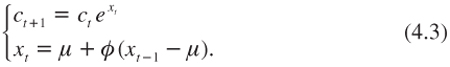
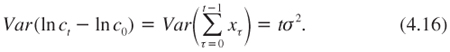
Up to this point, for the sake of simple notation, we have referred to r as “the” discount rate. However, if r is maturity varying it should be indexed by the maturity of the cost or benefit to be discounted. In fact, the general pricing formula (3.16) can now be rewritten:

The right-hand side of the equality depends in general upon t; therefore the left-hand side does as well. In fact, the pricing formula (4.1) provides the entire term structure of the discount rate.

Before going into further detail, it is helpful to develop an intuition of the determinants of this term structure. As has been seen before, the discount rate is determined by two competing effects: the wealth effect and the precautionary effect. Over two different time intervals, looking forward from the present to two different points in time, t and t′ > t, the intensity of each of these two effects may differ. This implies differing discount rates should be applied to cash flows occurring in period t to those occurring in period t′. Changes in the intensity of the wealth effect and the precautionary effect therefore form the shape of the term structure.

A FLAT TERM STRUCTURE

The simplest case arises when the growth rate is a constant g, now and forever. Assuming constant relative risk aversion γ, the pricing formula (4.1) implies that

The term structure is completely flat. Consumption increases exponentially with time, which implies that the intertemporal marginal rate of substitution, which is the discount factor exp(–r_tt), must decrease exponentially. This requires that the discount rate r_t is constant.

THE CASE OF DIMINISHING EXPECTATIONS

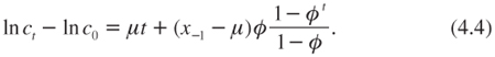
Suppose that, as in the simplest case just presented, there is certainty over the evolution of the economy. However, contrary to the previous paragraph, let us assume that the growth rate is not constant over time. Suppose that the growth rate decreases at a constant rate from x_–1 last year toward μ < x_–1 in the long run. More specifically, suppose that there exists a constant φ ∈ [0,1] such that

When φ equals 0, the growth rate goes immediately to μ in the next period, and remains there forever. When φ equals 1, the growth rate remains equal to x_–1 forever. When φ ∈]0,1[, the growth rate converges smoothly to μ. In short, φ measures the degree of persistence of the initial shock from x = μ to x = x_–1. In any case, we obtain that

In this certainty case with diminishing expectations, and assuming a power utility function, the pricing formula (4.1) can be rewritten as:

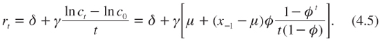
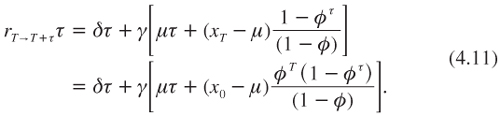
The first equality in (4.5) tells us that the wealth effect is proportional to the annualized growth of log consumption. This yields the following discount rates in the short and long terms:

In between, the efficient discount rate decreases smoothly at a constant rate. When expectations are diminishing, the term structure is downward sloping. This is because the wealth effect is strong for the short term, but reduces for longer time horizons.

There are two ideas that this simple dynamic of diminishing expectations illustrates. In the first story, the economy just faces standard business cycles. In that case, the preceding equations apply for the first few maturities t depending on the position in the cycle, either high (x_–1 > μ) or low (x_–1<μ). Remember, the socially efficient discount rate is also the equilibrium interest rate that one would observe on frictionless capital markets. Our analysis tells us that the shape of the yield curve, the term structure of the market yield to maturity of zero-coupon bonds, is a crucial source of information about what economic agents believe about the future dynamics of economic growth. A downward yield curve suggests people believe that the economy will experience a downturn in the future. On the contrary, an upward sloping yield curve is typical of an economy where growth is expected to accelerate, since the formulas (4.5) and (4.6) apply also when x_–1 < μ.

The same ideas apply for longer time horizons. In the second story, we may believe that the current level of growth is unsustainable, and that the economy will have to adapt to a lower, sustainable, growth rate μ. If one believes that the growth rate experienced by developed economies during the last two centuries is just unsustainable, this should be taken into account in the evaluation of long-term investment projects. The term structure of the discount rates should be decreasing. This will favor investment projects that have large positive benefits in the distant future in comparison to projects with more immediate benefits. In short, a decreasing term structure of discount rates supports sustainable development.

If the current growth rate of the economy is 2%, but its sustainable growth rate is believed to be only 0.5%, then applying the above pricing formula given, with δ = 0 and γ = 2, yields discount rates of 4% and 1% respectively for the short and long terms.

Economic growth is subject to business cycles. This should be accounted for when shaping the term structure of discount rates. In particular, discount rates should be revised periodically to take into account any changes in expectations about future growth in the short and medium terms. However, from our point of view, there is no argument which convinces us to believe that growth in the future will necessarily be smaller or larger than it is today. We do not side with catastrophists who believe that because of finite natural resources our economic growth is unsustainable. Just as there is a chance that future growth will be smaller than it is today, there is a chance that our society will experience a larger rate of growth—even larger than has been experienced since the beginning of the industrial revolution. This growth could be sustained by technological progress and the increasing de-materialization of economic activity. However, this does not mean that we should be unconcerned with the dynamics of growth into the distant future; quite to the contrary, as the next few chapters show.

DECREASING TERM STRUCTURE AND TIME CONSISTENCY

It is often suggested in the literature that economic agents are time inconsistent if the term structure of the discount rate is decreasing. This is not the case. What is crucial for time consistency is the constancy of the rate of impatience, δ, which is a cornerstone of the classic analysis presented in this book. We have seen that this assumption is compatible with a declining monetary discount rate. Other illustrations of this fact will be presented later on in this book. Let us re-examine this question under the simple framework of diminishing expectations as modeled by the deterministic dynamic process (4.3).

An agent is time consistent if the plan that is optimal at time t remains optimal for all future date t′ > t. To illustrate, consider an investment that costs one monetary unit at date T and that generates a single benefit k at time T + τ. Evaluating this project from date 0, investing is optimal if and only if its net present value is positive, that is, if:

This is equivalent to:

Assume that the agent’s consumption dynamics are represented by (4.3). The term structure r_t given by (4.5) should be used at date 0 to discount the cash flows in equation (4.8). Suppose that this condition is satisfied, so that, seen from today, it is optimal to implement the project at date T.

Consider now the decision problem at date T, when the time to invest in the project arrives. To solve this problem, we need to determine the discount rate that should be used at date T to discount the cash flow k occurring τ periods later. Let r_T→T+τ denote this discount rate. Seen from date T, it is optimal to invest in the project if and only if:

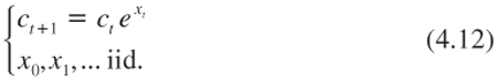
The problem of time consistency is about whether conditions (4.8) and (4.9) are equivalent, independent of k. Obviously, this requires that –r_T→T+ττ = r_T T – r_T+τ (T+τ). At date T, the level of x_T equals:

Duplicating the analysis presented in the previous section to the context of date τ implies that:

It is straightforward to check that this is equal to r_TT – r_T+τ(T+τ), which implies that the decision criterion to be used at date T is consistent with the one to be used at date 0. The decision process is thus perfectly time consistent, even though the term structure of discount rates is not flat.

RANDOM WALK

For uncertain future growth rates, the simplest assumption that can be made is that they follow a random walk. This means that the growth rate observed this year does not provide any information about the growth rate that will be experienced in the future. More specifically, suppose that the growth rate of the economy follows an independent and identically distributed (iid) process over time:

This implies that the pricing formula (4.1) can be rewritten as:

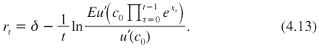
To keep things simple at this stage, consider the case of a power utility function with relative aversion γ. Using independence, equation (4.13) can then be rewritten as:

Because the process is iid, this can be rewritten as:

Thus, in the case of power utility functions and an iid process for the growth rate of the economy, the term structure of the efficient discount rate is completely flat. In the special case of a normal distribution for x, the extended Ramsey rule (3.23) gives us the level of this constant discount rate. This result can be found for example in Hansen and Singleton (1983).

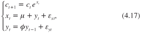
This case, which is the discrete version of a Brownian motion for the growth of the economy, serves as a benchmark for the analysis of the term structure of discount rates. It is therefore important to understand its nature. When the growth rate of the economy follows a random walk with a constant positive trend, the wealth effect goes up exponentially with the time horizon. If g = 2%, one expects to be 2% wealthier next year, and 5000% wealthier in 200 years. This exponentially increasing wealth effect justifies taking an exponentially decreasing discount factor. This requires a constant discount rate. Similarly, the random walk in the growth rate entails an exponentially increasing level of uncertainty about future consumption. This is equivalent to a linearly increasing variance for ln c_t. Indeed, it follows that:

The exponentially increasing precautionary effect that this implies should impact the discount factor exponentially. In other words, it should affect the discount rate uniformly with respect to the time horizon. Combining these two elements implies that the term structure of discount rates is flat.

A SIMPLE EXTENSION: MEAN-REVERTING GROWTH PROCESS

Following Bansal and Yaron (2004), for example, the two growth processes that have been considered in this chapter can be combined in the following simple model:

For some initial state characterized by y–1, where ε_xt and ε_yt are independent and serially independent with mean zero and variance and , respectively. The state variable y_t exhibits some persistence. As earlier, parameter φ, which is between 0 and 1, represents the degree of persistence in the expected growth rate process. When ε_x and ε_y are uniformly zero, this model is equivalent to the story of deterministic “diminishing expectations.” When φ is zero, the model returns to a pure random walk.

This autoregressive model of order 1—an AR(1)—illustrates the notion of mean-reversion. Suppose that the expected growth rate equals its historical level μ(y_–1 = 0), and that a positive shock ε_y0 affects the expected growth rate between dates 0 and 1, so that y₀ is larger than 0. Contrary to a random walk, this shock will have some persistence. For example, the expected growth rate between dates t and t + 1 will be Ex_t|ε_y0 = μ + φ^tε_y0 However, in the long run, the expected growth rate will revert to the mean. But at each date, a new persistent shock may affect the growth rate of the economy, in addition to the pure noise ε_xt.

The efficient term structure is determined in this case by characterizing the distribution of c_t. By forward induction of (4.17), it follows that:

The ε terms are assumed to be normally distributed; therefore so too is lnc_t–lnc₀. Its mean is the sum of the first two terms in the right-hand side of equality (4.18). Its annualized variance equals:

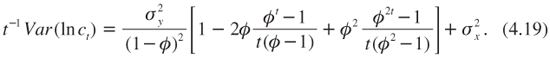
Observe that the annualized variance of log consumption tends to , which is larger than the short-run uncertainty measured by Var x₀ = . The long-run risk is increasing in the degree of persistence of shocks on the expected growth rate of consumption. This is because of the positive serial correlation in growth rates. More generally, the analysis of the right-hand side of (4.19) shows that the annualized variance of future log consumption goes up smoothly from to when t goes from 1 to infinity.

Suppose that u is a power function with relative aversion γ. The pricing formula (4.1) can therefore be rewritten as:

The normality of lnc_t–lnc₀ means that lemma 1 can be used to obtain that:

Finally, using the properties of the mean and variance of log consumption, the term structure of the discount rate can be characterized as follows:

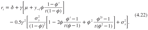
This equation can be rewritten as:

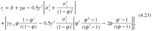
Observe that the last bracketed term of this equation is the only one that depends upon t and that it vanishes when t tends to infinity. It is this transitory term which shapes the term structure. The first three terms in (4.23) determine the long-term discount rate. Indeed, it yields:

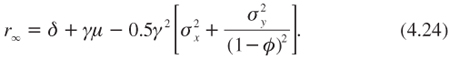
The long-term wealth effect is still measured by gm. The long-term precautionary effect is increasing in φ, therefore this effect is magnified by persistence. It can be concluded that if shocks on the growth rate of the economy are persistent, the rate at which very distant cash flows should be discounted is reduced. This is because of the increased long-term risk that the positive correlation of growth rates generates. To make this more precise, consider experts who believe that the growth rate of our economy follows a random walk. In order to estimate the efficient discount rate, they would use observations of past growth rates to estimate μ and σ. In particular, they would use the observed volatility of the growth rate to estimate s. With a large data set, they would obtain for the variance of changes in log consumption. Therefore, using the extended Ramsey rule, the recommendation would be a flat discount rate given by:

which is obviously larger than r_∞. In fact, by proceeding in this way, experts would provide the correct answer, but only for the short-term discount rate, and only when the past growth rate of the economy was equal to its historical mean (y_–1 = 0).

The term structure is given by the last term in equation (4.23). The part of that term including y_–1 corresponds to the “diminishing expectations” story that was explained earlier in the chapter. It yields a decreasing shape for the term structure if the economy is currently experiencing a growth rate above its historical mean. This effect is switched off by assuming that y_–1 = 0. In that case, the second term inside the brackets in (4.23) tells us how the discount rate goes down from the short-term rate r₁ given by (4.25) to r_∞ < r₁. The annualized variance of log consumption is increasing with the time horizon when there is persistence. Contrary to the pure Brownian case, this gives a decreasing term structure.

Let r_t→t+1 denote the rate that should be used at date t to discount cash flows occurring at date t+1. This is the short-term interest rate. Notice that the short-term interest rate in this model also follows an AR(1) process since using the pricing formula (4.21) for t = 1 yields

Vasicek (1977) was interested in determining the shape of the yield curve by using the standard arbitrage method in finance under the assumption of an AR(1) for the short-term interest rate. He got equilibrium interest rates for different maturities that are equivalent to formula (4.22). The degree of persistence φ is the same for economic growth and for the short-term interest rate. This is interesting because the degree of persistence of the latter has been well documented in the literature on the term structure of the interest rate. One important critique that has been made regarding Vasicek’s model is that the short-term interest rate expressed by (4.26) can become negative. This is a problem if a predictive model for the equilibrium interest rate is wanted, since the interest rate must be nonnegative (otherwise consumers will prefer to hold cash). This critique does not hold for our normative analysis. It may indeed be efficient to use a negative discount rate, in particular when a significant economic depression is predicted for the future.

Bansal and Yaron (2004) consider the following calibration of the model, using annual growth data for the United States for the period 1929–1998. Taking a month as the unit period, they obtained μ = 0.0015, σ_x = 0.0078, σ_y = 0.00034, and φ = 0.979. Using this φ yields a half-life for shocks of 32 months. This implies that the model is useful to justify differences in discount rates for maturities expressed in years, but not really for maturities expressed in decades or centuries. In other words, Vasicek’s model and mean-reversion in the growth rate are useful to explain the term structure of interest rates for maturities that are treated by financial markets, up to two or three decades.

Figure 4.1 describes how the term structure of interest/discount rates evolves along the business cycle. In addition to the Bansal-Yaron’s parameter values given earlier, it is assumed that the rate of impatience is δ = 0 and relative aversion is γ = 2. Three term structures are represented in this figure. When the recent growth rate is exactly at its historical mean (y₀ = 0, which corresponds to an annual growth rate of 1.8%), the yield curve is decreasing. This slope describes the increasing precautionary effect coming from the increasing annualized variance of future log consumption due to the persistence of shocks. During a downturn (illustrated by a low growth rate y₀ = –0.1%/month, which corresponds to an annual growth rate of 0.6%), the yield curve is upward sloping. This shape is mostly expressing an accelerating wealth effect generated by rising growth expectations, which are rising because of mean reversion. On the contrary, when the economy is booming with y₀ = 0.1%/month (corresponding to an annual growth rate of 3%), the yield curve is decreasing because of diminishing expectations. The long-term interest rate is not affected by the business cycle because the long-term growth rate in this model is deterministic and long-term uncertainty remains constant.

Figure 4.1. The efficient discount rate (in %) as a function of the maturity t (in years). Using the month as the unit period, the parameter values are δ = 0, μ = 0.0015, σ_x = 0.0078, σ_y = 0.00034, φ = 0.979, and γ = 2.

SUMMARY OF MAIN RESULTS

1.  The shape of the term structure of discount rates is determined by the way the wealth effect and the precautionary effects evolve with the time horizon.

2.  When the growth rate of consumption is constant, then consumption increases exponentially, and the intertemporal rate of substitution, which is the discount factor, decreases exponentially. This requires that the discount rate is constant.

3.  The simplest extension of this to uncertainty is to assume that the growth rate of the economy follows a random walk. In that case, the variance of log consumption increases linearly, which yields an exponentially increasing precautionary effect for the discount factor. This justifies a constant precautionary effect on the discount rate, yielding a crucial result for the theory of efficient discount rates: When the growth rate of the economy follows a random walk and when relative aversion is constant, the discount rate should be independent of the maturity of the project to be evaluated.

4.  A simple extension of the random walk for the growth rate of the economy is when the growth rate follows an autoregressive process of order 1. Mean-reversion has two consequences for the previous result. First, the term structure becomes sensitive to the business cycle. When the economy is booming, the short-term interest rate is large because of the wealth effect. However, the wealth effect becomes relatively less powerful in the longer term because the economy is expected to revert to a smaller growth rate. The result is a downward sloping term structure. The opposite effect arises in a downturn. The second effect of mean-reversion is to introduce some positive serial correlation in the growth rate. Compared to the case of a random walk, with correlation the long-term risk of the economy is magnified. This reinforces the precautionary effect over time, which acts to make the term structure downward sloping. This would be the case when the current growth rate of the economy is at its historical mean.

REFERENCES

Bansal, R., and A. Yaron (2004), Risks for the long run: a potential resolution of asset pricing puzzles, Journal of Finance, 59, 1481–1509.

Hansen, L., and K. Singleton (1983), Stochastic consumption, risk aversion and the temporal behavior of assets returns, Journal of Political Economy, 91, 249–268.

Vasicek, O. (1977), An equilibrium characterization of the term structure, Journal of Financial Economics, 5, 177–188.