8

A Theory of the Decreasing Term Structure of Discount Rates

This chapter completes part II of the book. It aims to provide a unified theoretical foundation to the term structure of discount rates. To do this it develops a benchmark model based on two assumptions: individual preferences toward risk, and the nature of the uncertainty over economic growth. We have shown that constant relative risk aversion, combined with a random walk for the growth of log consumption, yields a flat term structure for efficient discount rates. In this chapter, these two assumptions are relaxed by using a stochastic dominance approach.

The first step is to explore the link between the current long-term discount rate and expectations about what the future short-term discount rate will be.

THE CURRENT LONG DISCOUNT RATE AND FUTURE SHORT DISCOUNT RATES

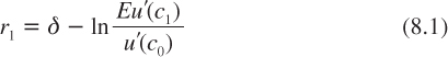
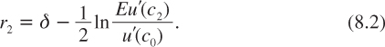
We limit the analysis to three equally distant dates, t = 0, 1, and 2. We assume that c₀ is known. At date t = 0, the short and long discount rates are, respectively

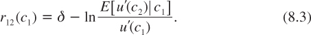
Suppose now that we are at date t = 1, with a realized level of consumption c₁. At that date under that state of nature, one should use a short rate denoted r_1→2(c₁). to discount a sure cash flow occurring one period later at date t = 2. To keep the notation simple, we write r_1→2 = r₁₂. This future short rate is as usual characterized by the following equation:

We want to link these three rates r₁, r₂, and r₁₂. This can be done by rewriting equation (8.2) as follows:

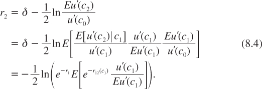
This implies that

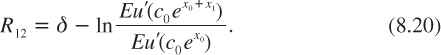
where R₁₂ is defined as follows:

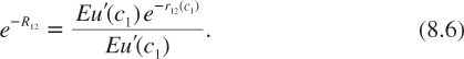
Equation (8.5) tells us that the long rate today is the average of the short rate r₁ today and R₁₂. Observe that the discount factor exp(–R₁₂) is the risk-neutral expectation of the future discount factor exp(–r₁₂(c₁)), using the risk-neutral probabilities for the distribution of the states of nature at date t = 1. Rate R₁₂, measured at date t = 0, depends upon the uncertainty about the immediate growth rate and upon the correlation of this growth rate with the interest rate that will prevail in the future. R₁₂ can also be interpreted as the certainty equivalent of the future short rate r₁₂. To keep terminology simple, let us refer to R₁₂ as the forward interest rate. It lies somewhere between the smallest and the largest possible future short rates. Using equations (8.3) and (8.6), R₁₂ can be rewritten as

It should not be a surprise that the discount factor to be used at date 0, to evaluate a transfer of consumption from date 1 to date 2, is equal to exp(-δ)Eu′(c₂)/Eu′(c₁). Evaluated today, this is indeed the marginal rate of substitution between c₁ and c₂. Remember that, by the first theorem of welfare economics, the efficient discount rate is also the equilibrium interest rate in a frictionless economy. In the same spirit, R₁₂ is the equilibrium forward interest rate, that is, the rate of return for a credit contract at date 0 offering a loan at date 1 with maturity at date 2.

Equations (8.5) and (8.6) also describe the links between current long rates and expectations about future shorter rates. It states that the following two investment strategies have the same effect on the expected utility at date 1. Under both strategies, consumption is reduced by ε at date 2 to fund an investment to increase consumption at date 1.

The first investment strategy is safe. It consists of borrowing long to invest short. More specifically, εexp(–2r₂) is borrowed at date 0, which requires a reimbursement of ε at date 2. This loan is used at date zero to invest in a short bond that yields a sure payoff ε exp(–2r₂)exp(r₁) at date 1. The increase in utility at date 1 is thus equal to that marginal sure increase in consumption multiplied by Eu′(c₁). The second investment strategy is risky. It consists of borrowing ε exp(–r₁₂) at date 1 that requires the same reimbursement ε at date 2. Seen from date 0, this is a risky strategy because the increased consumption at date 1 will depend upon the prevailing short-term rate r₁₂(c₁) at date 1. The increase in expected utility at date 1 is given by εEexp(-r₁₂)u′(c₁). At equilibrium, the two strategies must have the same effect on welfare. The following condition must therefore be satisfied:

which is equivalent to equation (8.4), which in turn yields property (8.5). This simple arbitrage argument explains why the long rate today must increase when investors expect the future interest rate to go up. It also explains the role of risk aversion in this relationship.

A vast literature on the term structure of interest rates has examined these interactions. Until seminal works by Vasicek (1977) and Cox, Ingersoll, and Ross (1985), economists based their analysis on the “Pure Expectations Hypothesis,” which states that the long rate today is the mean of the sequence of current and future short rates. Cochrane (2005, section 19.2) provides a useful analysis of this approach. It is similar to equations (8.5) and (8.6), but with a linear utility function u in (8.6). In spite of its inappropriate assumption of risk neutrality, this theory is compatible with the crucial idea that the current long rate tells us something about the investors’ expectation about the future rates.

DECREASING TERM STRUCTURE

There are two ways to write the condition that the long rate is smaller than the short one: r₂ ≤ r₁. First, from property (8.5), it is the case if the current short interest rate, r₁, is larger than the forward rate R₁₂:

Second, conditions (8.1) and (8.2) can be used more directly to get that r₂ is smaller than r₁ if:

which requires that:

Of course, given equations (8.1) and (8.7), these two approaches yield exactly the same condition for a decreasing term structure.

THE CASE OF AN IID DYNAMIC GROWTH PROCESS

In this section, the case in which the log of consumption exhibits no serial correlation is examined. What is sought is the condition on u that yields a decreasing term structure. Let x_t = log c_t+1 – log c_t denote the change in log consumption between dates t and t + 1. We assume that (x₀, x₁) are iid. It is easier to use variable Y_t = exp(x_t) = c_t+1/c_t, which is the relative change in consumption between dates t and t+1. Condition (8.11) for a decreasing term structure can therefore be rewritten as follows:

Let us first consider the special case of power utility functions with u′(c) = c^-γ. That condition is then equivalent to

Because y₀ and y₁ are independent, the left-hand side of this inequality equals , which in turn is equal to the right-hand side of (8.13) since y₀ and y₁ are identically distributed. We conclude that condition (8.13) holds as an equality, which implies that the term structure of discount rates is flat.

Under constant relative risk aversion, the short-term rate r₁₂ is independent of c₁. Indeed, from (8.3), we have that

It is a crucial property of the power utility function that the equilibrium interest rate is independent of the level of economic development. There is empirical support for this independence. During the twentieth century, GDP per capita was multiplied by a factor around 7 in the developed world, but no clear trend for the short-term interest rate has been observed. This is illustrated in figure 8.1, in which the series of short-term real interest rates between 1900 and 2006 in the United States is drawn. This argues in favor of constant relative risk aversion. If, in addition, expectations remain stable over time, implying that y₀ and y₁ are identically distributed, then comparing (8.14) and (8.1) implies that r₁ = R₁₂ = r₁₂. In turn, this implies that the term structure is flat.

Let us relax the assumption that relative risk aversion is constant. Instead, the case where r₁₂ is decreasing with c₁ is examined. From (8.3), this is the case if f(c₁) is increasing in c₁ where:

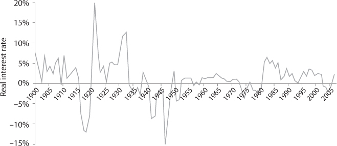
Figure 8.1. Real Bill rates in the United States in the twentieth century.
Source: Morningstar France.

Derivating with respect to consumption:

which is positive if:

This is equivalent to:

where R(c) = –c(c)/u′(c) is relative risk aversion. Suppose that consumption never falls (y₁ is almost surely larger than unity). If relative risk aversion is decreasing, this implies that R(cy₁) is smaller than R(c) almost surely. This implies that condition (8.18) always holds. Therefore, under the assumption that consumption never falls, decreasing relative risk aversion implies that the future short-term rate r₁₂ is decreasing in c₁. This implies that r₁₂(c₁) is almost surely less than r₁₂(c₀). Under the assumption that y₀ and y₁ are iid, this also means that r₁₂(c₁) is almost surely less than r₁. So is its certainty equivalent R₁₂. By equation (8.5), this implies that r₂ is less than r₁. Thus, when consumption never falls and growth exhibits no serial correlation, decreasing relative risk aversion is sufficient for a decreasing term structure. This condition is also necessary if we do not specify the distribution of y₁ with support in [1,+∞[. This result is in Gollier (2002a, 2002b).

In figure 8.2, we draw the term structure of discount rates in the special case of a modified power function with a minimum level of subsistence k:

This function is increasing and concave in its domain ]k,+∞[. Parameter k is interpreted as a minimum level of subsistence since when consumption goes to the level k, utility goes to –∞. It is easily checked that R(c) = γc/(c – k) under this specification. The function is decreasing in its relevant domain. It tends to infinity when consumption approaches the minimum level of subsistence, and it converges to γ for large consumption levels.

Let us normalize k to unity and consider c₀ = 2 as a benchmark. It is also assumed that the growth rate of the economy is a sure 2% per year, and that γ = 1, so that, as assumed elsewhere in this book, the relative risk aversion today is R(2) = 2. Using the Ramsey rule, which states that the interest rate net of the rate of impatience—which is assumed to be 0%—must be equal to the product of relative risk aversion and the growth rate of consumption. A short discount rate of 2 × 2% = 4% is obtained. For very long maturities, the relevant R to be used in the Ramsey rule is R(+∞) = 1, which yields a long discount rate equaling 1 × 2% = 2%.

In figure 8.2, current consumption c₀ is taken to be 20%, 50%, or 100% larger than the minimum level of subsistence. figure 8.2 therefore also depicts the situation for less developed countries whose GDP per capita is closer to the minimum level of subsistence. For the case where c₀ = 1.2, the marginal utility of consumption is considerably larger today than in the benchmark case, which implies that reducing today’s consumption to invest for the future is a lower priority. This takes the form of a large discount rate r = R(1.2)×2% = 12% in the short run. This may explain why poorer countries are observed to be more short-termist in relation to various public investments such as education or infrastructure.

Under the assumption of never decreasing consumption, the term structure is decreasing with maturity if and only if relative risk aversion is decreasing with wealth. The intuition for this result is simple. The intensity of the wealth effect is proportional to R, which measures the aversion to intertemporal inequality. In a growing economy, this effect decreases over time when R is decreasing with wealth. This implies that interest rates will tend to go down in the future. This generates in turn a decreasing term structure of interest rates today. However, this approach is at odds with the empirical observations that the short-term interest rate is independent of the degree of economic development. In the next section, an alternative approach is considered to justify the type of downward sloping term structure which would be consistent with the analysis presented in the second part of the book.

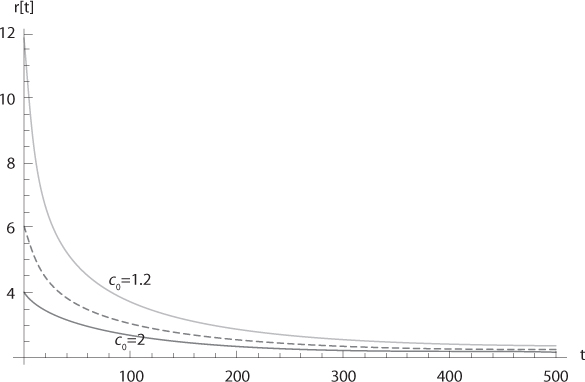
Figure 8.2. The term structure of discount rates with δ = 0%, x_t = 2%, u′(c) = (c = 1^-1), c₀ = 1.2, 1.5, and 2.

A CONCEPT OF CONCORDANCE: “LARGE VALUES OF X₁ GO WITH LARGE VALUES OF X₂”

This section is devoted to the analysis of the impact on the forward interest rate of serial correlation in the growth rate of the economy. Up to now in this chapter, we examined the case of random walk for the change in log consumption, and we relaxed the assumption that relative risk aversion is constant. In the remainder of this chapter, we examine the role of serial correlation in the change of log consumption.

The forward rate is characterized by the following equality:

This equation makes explicit that serial correlation in the growth of log consumption matters, as illustrated in the previous chapters. In the special case without serial correlation and constant relative risk aversion, we know that R₁₂ = r₁₂ = r₁, so that, according to condition (8.5), the term structure is flat. From now on in this chapter, the assumption of serial independence is relaxed in a framework in which there is no a priori specification of the utility function u.

In the general expected utility model, the coefficient of correlation between two random variables as x₁ and x₂ is usually insufficient to characterize the role of the statistical relationship on an expectation as Eu′(c₀e^x₀+x₁), that is, on the term structure of discount rates. The full joint distribution function is generally required to determine the forward discount rate. Following Tchen (1980) and Epstein and Tanny (1980), the idea that “greater values of x₁ go with greater values of x₂” is now formalized. To do this, consider an initial distribution function F for the pair of random variables (x₁, x₂), with F(t₁, t₂) = P[x₁ ≤ t₁ ∩ x₂ ≤ t₂]. Consider another pair of random variables with cumulative distribution function (cdf) . A “marginal-preserving increase in concordance” (MPIC) is defined as any transformation of distribution F into distribution that takes the following form: Consider two pairs (t₁, t₂) and(₁₂) such that ₁ > t₁ and ₂ > t₂ obtained from F by adding probability mass ε in a small neighborhood of (t₁, t₂) and (₁, ₂), while subtracting probability mass ε in a small neighborhood of (t₁, ₂) and (t₁, ₂). This is depicted in figure 8.3.

This MPIC clearly increases the correlation between the two random variables, without affecting the marginal distributions of the two random variables. Observe also that the new cdf, , obtained through a MPIC uniformly raises the cdf: for all (t₁, t₂), (t₁, t₂) ≥ F(t₁, t₂). Following Tchen (1980), this inequality defines the notion of “more concordance” for any two cdfs F and with the same marginals (t₁,+∞) = F(t₁,+∞) ∀t₁ ∈ and (+∞, t₂) = F(+∞, t₂) ∀t₂ ∈ :

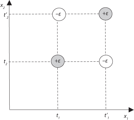
Figure 8.3. Transfer of probability mass in a marginal-preserving increase in concordance.

A more concordant cdf concentrates more probability mass in any South-West and North-East quadrangles of ². Tchen (1980, theorem 1) and Epstein and Tanny (1980) show that two cdfs with the same marginals can be ranked by this notion of increasing concordance if and only if the more concordant cdf can be obtained from the less concordant one through a sequence of MPICs. It is interesting to observe that, by dividing both sides of the inequality in (8.21) by (t₁,+∞) = F(t₁,+∞), this definition is equivalent to

This is in turn equivalent to the following definition of an increase in concordance, which relies on the notion of First-order Stochastic Dominance (FSD):

This can be seen clearly in figure 8.3. Suppose that the MPIC represented in this figure is undertaken, and that the information is received that x₁ is smaller than some t ∈]t₁₁[. What remains visible to the left of t is the downward transfer of probability mass that happens in the neighborhood of t₁, which is a FSD deterioration in the conditional distribution of x₂. Conditional on the fact that x₁ is smaller than any threshold t₁, the probability distribution of ₂ is a deterioration of x₂ in the sense of FSD. This means that some probability mass of this conditional distribution is transferred from the high values of x₂ to the lower ones. Under the new distribution, there is always more probability mass in the left tail of the distribution of x₂ | x₁ ≤ t₁.

In words, this means that the present and the future changes in consumption are more strongly correlated after a sequence of MPICs. Bad news in the first period is bad news for the second period’s distribution of consumption. In the statistical literature, this notion is referred to as the “stochastic increasing positive dependence,” because x₂ is more likely to take on a larger value when x₁ increases (see for example Joe 1997). It is closely related to the notion of “positive quadrant dependence” proposed by Lehmann (1966). Gollier (2007) was too restrictive in identifying the notion of more concordance with respect to a pair of independent random variables with the stronger condition of “positive FSD dependence” that requires that x₂ | x₁ = t₁ be ordered by first-degree stochastic dominance.

CONCORDANCE AND SUPERMODULARITY

Suppose that we are interested in the effect of an increase in concordance on the expectation of some function h:² → . Let us first consider the effect of an elementary MPIC defined by pairs (t₁, t₂) and (₁,₂) such that ₁ > t₁ and ₂ > t₂, as in figure 8.3. Obviously, this MPIC increases the expectation of h if and only if

Because the two pairs (t₁, t₂) and (₁,₂) are arbitrary, this condition must hold for all such pairs such that ₁ > t₁ and ₂ > t₂. This condition is necessary and sufficient for an increase in concordance to raise the expectation of h because any increase in concordance can be expressed as a sequence of MPICs. It happens that this condition is well-known in mathematical economics. It is referred to as the “supermodularity of h.”

If h represents a von Neumann-Morgenstern utility function in ², taking condition (8.24) and dividing both sides of the inequality by 2, implies that one would prefer a lottery yielding payoff (t₁, t₂) or (₁,₂) with equal probabilities. to another lottery yielding payoff (₁, t₂) and (t₁,₂) with equal probabilities. This would be the case, for example, for complement goods where x₁ and x₂ are respectively the number of left and right shoes in the consumption bundle. Condition (8.24) thus defines a notion of complementarity between x₁ and x₂. Two goods are complements if the marginal utility of the first is increasing in the consumption of the second, that is, if the cross derivative of the utility function is positive.

Observe that if h is twice differentiable, replacing (₁,₂) by (t₁ + dx, t₂+dy), inequality (8.24) is equivalent to

for all dx > 0 and dy > 0. A simple integration argument implies that when h is twice differentiable, the supermodularity of h is equivalent to its having a positive cross derivative.

The following lemma summarizes the findings so far. The formal proof of the lemma is in Tchen (1980), Epstein and Tanny (1980), or Meyer and Strulovici (2011).

Lemma 2: Consider a bivariate function h. The following conditions are equivalent:

• For any two pairs of random variables (x₁, x₂) and such that is more concordant than (x₁, x₂) Eh ≥ Eh(x₁, x₂).

• h is supermodular.

Moreover, assuming that h is twice differentiable, Tchen (1980, theorem 2) shows that

This can be obtained by a double integration by parts. By the definition (8.21) of an increase in concordance, we see that equation (8.26) provides a simple proof for this lemma.

An immediate application of the lemma is to apply it to function h(x₁, x₂) = x₁ x₂, which is supermodular. Lemma 2 tells us that an increase in concordance raises the expectation of h. Since the marginal distributions are preserved because E_i = Ex_i, this shows that an increase in concordance necessarily raises the covariance between the two random variables.

THE EFFECT OF AN INCREASE IN CONCORDANCE OF ECONOMIC GROWTH ON THE FORWARD DISCOUNT RATE

There is a clear link between the notions of supermodularity and of an increase in concordance. Consider two dynamic processes for the growth of consumption (shown in figure 8.4).

The perfect positive concordant pair of random variables in (a) is obtained from the perfect negative concordant pair in (b) through a MPIC transferring all the probability mass from the upward diagonal of the rectangle to the downward one. In the two cases, the marginal distributions of x₁ and x₂ are the same: x_t ~ (1%,1/2; 3%,1/2), but they are perfectly positively correlated in case (a), whereas they are perfectly negatively correlated in case (b).

Define

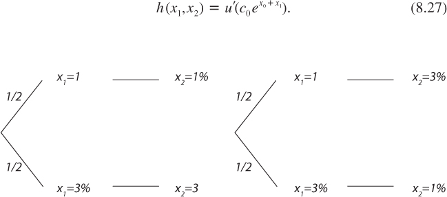
Figure 8.4. Illustrations of perfect positive and negative concordance.

Equation (8.20) tells us that the forward discount rate R₁₂ is negatively affected by an increase in concordance if Eh is positively affected by it. Using lemma 2, this requires that h is supermodular. It follows that

where c₂ = c₀exp(x₁+x₂) consumption atdate t = 2 and P(c) = –c(c)/ is the index of relative prudence. This proves the following proposition:

Proposition: Any increase in concordance in the growth of log consumption reduces the forward discount rate if and only if relative prudence is uniformly larger than unity.

By equation (8.5), P ≥ 1 is also necessary and sufficient to reduce the long discount rate. Now, remember that combining the assumption of iid (x₁, x₂) with constant relative risk aversion implies a flat term structure. Remember also that constant relative risk aversion implies that relative prudence is also constant and is equal to relative risk aversion plus one. Thus, when relative risk aversion is constant, it must be that relative prudence is larger than unity. Thus, under this assumption, the term structure of discount rates is decreasing if, for the same marginal cdf, the growth process exhibits more concordance than in the case of serial independence.

The intuition for this result is based on the observation that the second moment of c₂ is the expectation of a supermodular function of (x₁, x₂). Indeed, function

is supermodular. It implies that an increase in concordance for the change in log consumption tends to raise the variance of c₂. This reduces the forward discount rate under prudence. However, observe also that the expectation of c₂ is increased by the concordance in (x₁, x₂), since h(x₁, x₂) = c₀exp(x₁ + x₂) is supermodular. This wealth effect goes against the precautionary effect. This explains why positive prudence is not sufficient to determine the sign of the effect of an increase in concordance of log consumption. Using lemma 2, it is easy to check that positive prudence is necessary and sufficient when the dynamic process of consumption exhibits more concordance than in the case of independence. Heinzel (2011) shows how to generalize this analysis to higher orders of stochastic dependence and to higher derivatives of the utility function.

UNIFIED EXPLANATION FOR A DECREASING TERM STRUCTURE OF DISCOUNT RATES

The stochastic processes that we examined in chapters 4 (mean-reversion), 5 (Markov switches), and 6 (parametric uncertainty) exhibited some forms of stochastic dependence in serial changes of log consumption. Their common feature is the increased concordance of successive changes in log consumption compared to the case of a random walk. This provides a common underlying explanation for the decreasing term structure derived for each of these models. The simplest illustration of this is obtained in the case of Markov switches. Suppose that there are two regimes, one with a sure growth rate of 2%, and one with no growth. There is a 1% probability to switch from one regime to the other every year. Figure 8.5 (left) describes the probability distribution for the growth rate in the first two years, assuming that one experienced a good state in the previous year. Figure 8.5 (right) describes the probability distribution with no serial correlation, but with the same marginal probabilities as in the original distribution on the left. We see that the Markov-switch process is more concordant than in the case of independence, since it is obtained from the latter through a MPIC of a probability mass of 0.97%.

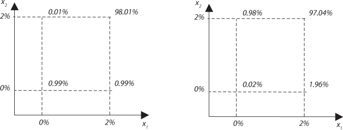
Figure 8.5. A two-state Markov process (left) that is more concordant than in the case of independence (right). The switching probability in each period is 1%.

Alternatively, consider the mean-reverting process x_t + ₁ = φx_t + (1 – φ) µ + ε_t, with φ ∈[0,1] and where ε_t is normally distributed with mean 0 and volatility σ. We have seen in 2. chapter 4 that this yields a decreasing term structure under CRRA when x₀ = µ, which guarantees that Ex₁ = Ex₂. In figure 8.6, the iso-density curves of (x₁, x₂) are depicted, together with the curves for the pair of independent random variables with the same marginal distributions (x₁ ~ N(µ, σ²) and x₂ ~ N(µ, (1 + φ²)σ²)). We clearly see that the pair exhibiting mean-reversion exhibits more concordance than the corresponding independent pair. A similar observation can be made for the case of parametric uncertainty.

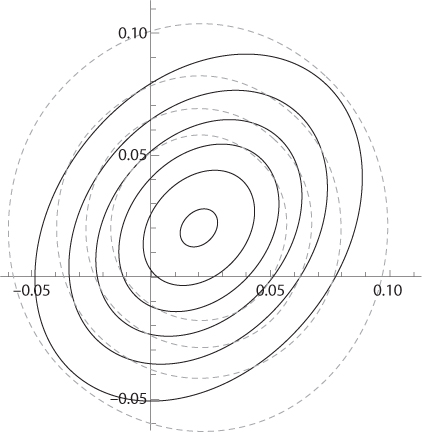
Figure 8.6. Iso-density curves in the case of mean-reversion with µ = 2%, σ = 3.6%, and φ = 0.3. The dashed curves correspond to the iso-density curves of the pair of random variables with the same marginal distributions.

SUMMARY OF MAIN RESULTS

1.  By a simple arbitrage argument, the term structure of interest rates is decreasing if the short-term interest rate is larger than the forward rate. The forward discount factor is the risk-neutral expectation of the future short-premium.

2.  If the growth rate of consumption follows a random walk but is always non-negative, the forward interest rate is smaller than the short rate if and only if relative risk aversion is decreasing. In this context, this is also necessary and sufficient for a decreasing term structure. This may explain a greater degree of short-termism in public investments observed in developing countries whose citizens are close to their subsistence level of consumption.

3.  Stochastic models of economic growth with mean-reversion, Markov switches, and parametric uncertainty all exhibit some forms of positive statistical dependence of successive growth rates. Because this tends to magnify the long-term risk, it is the driving force of the decreasing nature of the term structure. We formalize this idea by the notion of concordance, in which probability masses are transferred in favor of more concordant growth rates without changing the marginal distributions. This family of changes in the joint distribution of growth rates reduces the forward rate and makes the term structure more downward sloping if and only if relative prudence is larger than unity.

REFERENCES

Cochrane, J. H. (2005), Asset Pricing. Revised Edition, Princeton: Princeton University Press.

Cox, J., J. Ingersoll, and S. Ross (1985), A theory of the term structure of interest rates, Econometrica, 53, 385–403.

Epstein, L. G., and S. M. Tanny (1980), Increasing generalized correlation: a definition and some economic consequences, Canadian Journal of Economics, 13, 16–34.

Gollier, C. (2002a), Discounting an uncertain future, Journal of Public Economics, 85, 149–166.

Gollier, C. (2002b), Time horizon and the discount rate, Journal of Economic Theory, 107, 463–473.

Gollier, C. (2007), The consumption-based determinants of the term structure of discount rates, Mathematics and Financial Economics, 1 (2), 81–102.

Heinzel, C. (2011), Term structure of interest rates under multivariate -ordered consumption growth, mimeo, Toulouse School of Economics.

Joe, H. (1997), Multivariate Models and Dependence Concepts, London: Chapman and Hall/CRC.

Lehmann, E. L. (1966), Some concepts of dependence, Annals of Mathematical Statistics, 37, 1153–1173.

Meyer, M., and B. Strulovici (2011), The supermodular stochastic ordering, Nuffield College, Oxford University.

Tchen, A. H. (1980), Inequalities for distributions with given marginals, Annals of Probability, 8, 814–827.

Vasicek, O. (1977), An equilibrium characterization of the term structure, Journal of Financial Economics, 5, 177–188.