2

The Ramsey Rule

In this chapter, we present the main argument in favor of a positive discount rate. In a growing economy, future generations will consume more goods and services than we do. In this context, investing for the future is equivalent to asking poor consumers to sacrifice more of their consumption for the benefit for wealthier people. Because of inequality aversion, one would be ready to do so only if the rate of return of these investment projects is large enough to compensate for the increased intertemporal inequalities that these projects would generate. The Ramsey rule quantifies this wealth effect.

WHY DO WE NEED A MODEL?

The most obvious way to determine the efficient discount rate is to make it equal to the rate of return on risk-free capital, as explained in chapter 1. This is referred to as the interest rate, which measures the opportunity cost of funds in the economy. This is certainly a good reference when the cash flows to be discounted occur in the next few months or years. However, in order to use financial markets to estimate the discount rate, it is necessary to observe the real rate of return for truly risk-free assets.

Most corporations and public institutions use as their discount rate the rate at which they can borrow on financial markets, or their Weighted Average Cost of Capital (WACC). Normally this rate contains a risk premium because their investment projects are risky, with cash flows that are correlated with systematic risk in the economy (see part IV of this book). It is often suggested that corporations and their shareholders use a rate of around 15% to evaluate their investment projects. This rate contains a risk premium. Therefore it is not what is referred to in this book as the discount rate, which is instead the rate at which a sure future benefit must be discounted to measure its present value.

The safest assets on the planet are bonds issued by governments in the western world. Those issued by the United States are the safest, but the recent crisis on sovereign debts reminds us that this safest asset is not risk-free, in particular for long maturities. However, the probability of default of U.S. Treasury bonds remains small, because of the extensive ability to tax U.S. citizens’ incomes. The nominal opportunity cost of risk-free capital is revealed by the rate of return on these bonds. Combined with an almost deterministic short-term inflation rate it is straightforward to calculate the real rate of return for short-term maturities. This provides a clever basis to fix the short-term discount rate.

In the longer term, the rate of return on government bonds with longer maturities provides a noisier signal about the cost of borrowing for a risk-free agent. There are increasing uncertainties surrounding inflation and the probability of default. These uncertainties imply that empirical data from financial markets are tainted with frictions, inefficiencies, and bubbles. In turn this implies a role for economic models which can be used to construct a scientific basis for the discount rate.

There is a further limitation to using rates of return on government bonds in the longer term. There does not exist, in any significant quantity on sufficiently liquid markets, bonds with maturities longer than thirty or fifty years. Moreover, as is well-known from the overlapping-generation models of the theory of growth, future generations cannot trade on present credit markets, which makes them intrinsically dynamically inefficient (Diamond 1977). Therefore, there isn’t any clear benchmark from financial markets to help determine the rate at which distant cash flows should be discounted. As a consequence, two of the three ways proposed in chapter 1 to estimate the discount rate are invalid for long time horizons.

In the following, an approach based on the welfare-preserving rate of return of saving is used, which will produce the famous Ramsey rule. This approach is sustained by the assumption that the investment project to be evaluated will be financed by a reduction of aggregate consumption rather than by a substitution from other investments, so that the discount rate is related to the marginal rate of substitution between current and future consumption. This can also be interpreted as an attempt to predict what the equilibrium interest rate should be in an economy with perfect financial markets and paternalistic investors. In other words, our aim is to price risk-free assets according to a welfare-compatible interpretation of the notion of sustainable development.

ADDITIVE TIME PREFERENCES

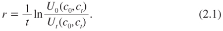
The previous chapter examined a simple sure investment project yielding only two cash flows—a cost today and a benefit at some specific date t. It was seen that the minimum (continuously compounded) rate of return that makes this project socially desirable is:

In the absence of financial market failures, this socially efficient discount rate is also the equilibrium yield to maturity of a zero-coupon bond with maturity t. In this chapter, this simple equation is calibrated. Two ingredients are required; the shape of the intertemporal utility function U, and the economic growth from c₀ to c_t ≥ c_0.

An important simplifying assumption is that U is additive with respect to time. Namely, it is assumed that there exist two functions, u and v_t from to such that

Equation (2.2) can be interpreted as follows: agents evaluate their intertemporal welfare by adding their immediate utility u(c₀), generated by consuming c₀, to the anticipated utility v_t(c_t), generated by consuming c_t in the future. This anticipated utility is independent of past consumption: the level of initial consumption c₀ has no effect on the utility of consumption at date t. This precludes the formation of consumption habits, any anticipatory feelings, or any emotional hysteresis. This assumption is important because it allows the two dates 0 and t to be isolated in the evaluation of the welfare-preserving rate of return on saving related to a benefit occurring at t. If there were some formation of consumption habits, the entire consumption plan between 0 and t would have an effect on the marginal value of consumption at date t. Similarly, if we would allow for anticipatory feelings, consumption levels after time t would matter to determine the utility associated with date t. The origin of the additively separable discounted utility function can be traced back to Samuelson (1937). Its axiomatic foundation was provided by Koopmans (1960).

EXPONENTIAL PSYCHOLOGICAL DISCOUNTING

Since Ramsey (1928), economists have made the assumption that agents are impatient. They value their future utility less than current utility. An immediate pleasure is preferred to an identical one that is experienced in the future. This impatience is modelled by assuming that there is a single function u that links the level of instantaneous consumption to the level of instantaneous felicity, and that lifetime utility is a discounted flow of current and future felicities. In other words, the additive specification (2.2) is considered in the special case with v_t (c) = exp(–δt)u(c) for all c. More generally with more than two periods, the intertemporal welfare function is assumed to be a weighted sum of the flow of future felicities, the weight associated to any maturity t being exponentially decreasing at a constant rate δ.

Parameter δ is the rate of pure time preference, or the rate of impatience. Some economists refer to it as the “discount rate,” which is a source of misunderstanding. Indeed, it is a discount rate, since it is used to discount the flow of future utility. However, it is not the discount rate in the usual sense, which is the rate used by economists to discount future cash flows. Of course, as is shown next, there is a link between the psychological discount rate δ and the monetary discount rate that is denoted by r in this book.

The choice of the exponentially decreasing function, f(t) = exp(–δt), for the utility discount factor relies on a simple argument of time consistency. Consider the same investment problem as in the previous chapter, with an initial cost to be incurred at date 0 and a benefit at date t. However, rather than examining the value of the project at date 0, suppose that it is examined at some date –τ < 0, before its implementation. Suppose that no new information about the quality of the project and about the environment of the investor is expected between –τ and 0. Time consistency requires that if it is optimal at date –τ to plan to invest at date 0, it is indeed optimal to invest when date 0 comes. Planning is rational. From the initial date –τ, the duration of time before enjoying utility u(c₀) is τ years, so that a discount factor exp(–δτ) must be attached to utility occurring at date 0. Similarly, the duration of time before enjoying utility at date t is τ + t years, so that a discount factor exp(–δ(τ + t)) should be used to discount utility from consumption at date t, u(c_t). It can be concluded that the intertemporal welfare function at date –τ can be written as

It can be observed that the objective function at date –τ is the product of a constant independent of the characteristics of the project, and of the objective function at date 0. Therefore, any project that raises the welfare U(c₀, c_t) as evaluated at date 0 also raises welfare when evaluated at date –τ. This guarantees time consistency. The exponential nature of the discount factor in the intertemporal welfare function guarantees that the relative “exchange rate” of utility for any pair of dates is insensitive to the passing of time. Other specifications for the utility discount factor, such as the hyperbolic one with f(t) = (1+at)^–1, induce time inconsistent behaviors. Strotz (1956) and Laibson (1997) provide interesting insights about the saving behavior of time-inconsistent consumers.

RATE OF IMPATIENCE

There is a simple way to estimate the rate of impatience δ. Suppose you believe that your income in the future will be the same as this year, and that you currently have no savings. What is the minimum interest rate that would induce you to save some of your current income? The answer to this question is called your welfare-preserving rate of return, which is defined by equation (2.1). Under the previous assumptions with c₀ = c_t, we obtain that U₀/U_t = exp(δt), so that r = δ. The rate of impatience is equal to the minimum interest rate that induces people to save when their income profile is flat.

There is no convergence among experts toward an agreed, or unique, rate of impatience. Frederick, Loewenstein, and O’Donoghue (2002) conducted a meta-analysis of the literature on the estimation of the rate of impatience. Rates differ dramatically across studies and within studies across individuals. For example, Warner and Pleeter (2001), who examined actual households’ decisions between an immediate down payment and a rental payment, found that individual discount rates vary between 0% and 70% per year! Thus, the calibration of δ is problematic if the objective is positive, that is, if one wants to explain real behaviors.

As long as consumption at date 0 and t concerns a given person, impatience is a psychological trait that economists should take as given. However, many experts in the field have questioned, from a normative perspective, the appropriateness of impatience for the evaluation of social welfare. Arrow (1999) cites various classical authors on this matter. The most well-known citation is from Ramsey (1928) himself: “It is assumed that we do not discount later enjoyments in comparison with earlier ones, a practice which is ethically indefensible and arises merely from the weakness of the imagination.” Many other distinguished economists can also be cited: Sidgwick (1890): “It seems … clear that the time at which a man exists cannot affect the value of his happiness from a universal point of view; and that the interests of posterity must concern a Utilitarian as much as those of his contemporaries”; or Harrod (1948): “Pure time preference [is] a polite expression for rapacity and the conquest of reason by passion.” Koopmans: “[I have] an ethical preference for neutrality as between the welfare of different generations.” Solow (1974): “In solemn conclave assembled, so to speak, we ought to act as if the social rate of pure time preference were zero.”

The general view is that a small or zero discount rate should be used when the flow of utility over time is related to different generations. The fact that I discount my own felicity next year by 2% does not mean that I should discount my children’s felicity next year by 2%. In fact, there is no moral reason to value the utility of future generations less than the utility of the current ones. As explained by Broome (1992), good at one time should not be treated differently from good at another, and the impartiality about time is a universal point of view. The normative doctrine is that the rate of time preference is zero. In later sections, this book takes a normative stand to set δ at zero. This is justified because the dominant role of the discount rate over the longer term is to allocate utility across different generations rather than within an individual’s lifetime. If one treats different generations equally, the only argument in favor of a positive rate of pure preference for the present is the possibility of extinction. For example, Stern (2007) uses a δ of 0.1% per year that is justified by the quite arbitrary assumption that there is a 0.1% probability per annum that humanity will disappear within the next twelve months.

A classical argument against a zero discount rate goes as follows. Consider the standard utilitarian social welfare function

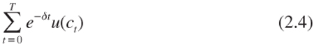
where the time horizon T of the social planner tends to infinity. If δ is zero, this social welfare function will be unbounded. Economists would find that problematic. For example, consider the problem of the optimal rate of extraction of a non-renewable resource. Because the objective function is unbounded, this problem could not be solved, or has multiple solutions. Macroeconomists and growth theorists would face a similar challenge. However, the problem of the discount rate does not require maximizing anything. The discount rate is the price of time that is compatible with a given consumption plan. It tells us what the changes in consumption are that improve intertemporal welfare, independent of whether the initial consumption plan is dynamically optimal or not. Thus, this argument of an undoubted social welfare function when δ = 0 and T tends to infinity is irrelevant for our purpose in this book.

AVERSION TO INTERTEMPORAL INEQUALITY OF CONSUMPTION

It was shown in the previous chapter that the concavity of the intertemporal welfare function U characterizes a preference for the smoothing of consumption over time. In the additive case examined here, this is translated into the concavity of the utility function u.¹ The local measure of the degree of concavity of the utility function u is defined:

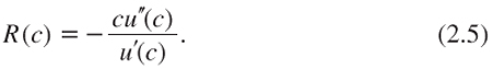
This index is hereafter referred to as the relative aversion to intertemporal inequality of consumption. To illustrate why, suppose that an individual’s consumption plan, (c₀, c_t), is unequally distributed over time. Suppose more particularly that future consumption is larger than current consumption: c_t > c₀. How much would the individual be ready to pay today to increase consumption by one unit in the future? This should be less than one unit for two reasons: impatience and aversion to consumption inequality. In the absence of both of these effects, the individual would be prepared to exchange one for one, as explained in the previous section. Let k be the maximum reduction in current consumption that is compatible with the unit increase in future consumption. It must satisfy the following indifference condition:

Assume that t = 1, and that δ and c₁ – c₀ are small. Using a first-degree Taylor approximation of u′(c₁) around c₀ and using the approximation exp(–δ) 1 – δ implies that:

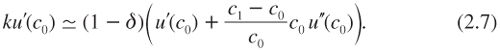
This can in turn be rewritten as:

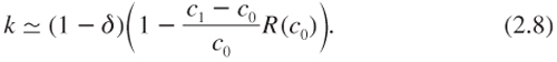
This equation can be used to estimate your relative aversion to intertemporal inequality R(c₀). Suppose that your rate of impatience is δ = 0, and that you anticipate an increase in future consumption of 10%. In spite of this increase, you are considering a sure investment which will transfer consumption to the future. What is the maximum reduction k of current consumption that you are ready to sacrifice, or invest, to increase future consumption by 1 dollar? The answer to this question gives us an estimation of your relative aversion to intertemporal inequality, since by (2.8), R(c₀) 10 – 10k. For example, answering 90 cents to the question yields a relative aversion R = 1, whereas an answer of 80 cents yields a relative aversion R = 2.

There is no consensus on the intensity of relative aversion to intertemporal inequality. Using estimates of demand systems, Stern (1977) found a concentration of estimates of R around 2 with a range of roughly 0–10. Hall (1988) found an R around 10, whereas Epstein and Zin (1991) found a value ranging from 1.25 to 5. Pearce and Ulph (1995) estimate a range from 0.7 to 1.5. Following Stern (1977) and the author’s own introspection, we will hereafter consider R = 2 as a reasonable value.

When different generations are concerned by the investment project to be evaluated, the choice of the discount rate entails interpersonal comparisons of utility. In that case, function U is interpreted as a social welfare function, and the concavity of u characterizes collective aversion to interpersonal inequality. Is the level of R affected by this shift in analysis? In this literature, it is generally assumed that our normative attitude toward consumption inequalities should not depend upon the nature of the comparisons of consumption levels. Under the common paternalistic view, one should evaluate the impact on social welfare of an intertemporal inequality of consumption exactly as if it would be an interpersonal inequality. The social evaluation should be impartial. It is claimed that the two problems are equivalent by nature. From a normative point of view, if one is ready to pay up to 80 cents to increase one’s own consumption by one dollar next year, in spite of an anticipated 10% increase in consumption, society should also be ready to sacrifice 80 cents of person A’s consumption in order to increase consumption by one dollar for person B, who is 10% wealthier than person A. Thus, it is maintained that R = 2 is a sensible level of relative aversion to inequality even in the intergenerational context.

THE POWER UTILITY

Economists and econometricians often limit their analysis by using a specific utility function in their model. They usually favor exponential, quadratic, logarithmic, or power utility functions. In this book, as in the modern theory of finance, the special case of the power utility function will be used most frequently:

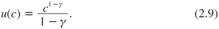
Parameter γ is positive and different from 1. When γ = 1, we take u(c) = ln(c), since it can be verified that the limit of (2.9) when γ tends to 1 is the logarithmic utility function. These utility functions are increasing and concave because u′(c) = c^–γ. Moreover, the index R of relative aversion to intertemporal inequality is a constant independent of c, and is equal to γ.

Using this utility function, we can re-examine the degree of realism of our assumption R = γ = 2 without relying on Taylor approximations as in the previous section. Consider an agent with utility function u(c) = – c – 1 and with δ = 0. Suppose that this person expects to double his consumption in the future. This implies that this person will be ready to give up as much as u′(c_t)/u′(c₀) = (c_t/c₀)^–2 = 0.25 dollar today to increase consumption by one dollar in the future. In the context of the reduction of inequalities, consider a society in which half of the population consumes twice as much goods and services than the other half of the population. If we assume a utilitarian social welfare function with this power utility function, one would find socially desirable to sacrifice as much as one dollar for each rich to increase consumption by 25 cents for each poor. If one would have considered a calibration with R = γ = 1, the ratio 1:4 should be replaced by a ratio 1:2. Readers can decide for themselves about the “right” level of γ from this type of introspective exercise.

The use of a power utility function is not an innocuous assumption. The constancy of the relative aversion means in particular that the answer k to the earlier question depends not on the initial absolute level of consumption, but only upon its growth rate. This implication can be challenged, in particular given the fact that there must be some positive minimum level of subsistence. If current income is at or above this minimum subsistence level, an individual would be entirely unwilling to transfer consumption to a future period, independent of the growth rate of consumption. This is not the case with function (2.9). In addition, this power utility function implies that the marginal utility tends to infinity when consumption tends to zero. Consider a future state of nature where consumption tends to zero. Specification (2.9) implies that one would be ready to sacrifice almost 100% of one’s current wealth in order to increase wealth in this future state by one dollar. This is not realistic. It is therefore necessary to be quite cautious in the use of the classical power utility model when there is the possibility of Armageddon scenarios.

THE RAMSEY RULE

It is time to bring together the different pieces discussed so far in this chapter. Rewriting equation (2.1), the efficient discount rate must be equal to

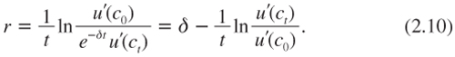
A Taylor expansion of u′(c_t) around c₀ yields

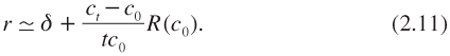
Equations (2.10) and (2.11) show that the socially efficient discount rate has two components. It is the sum of the rate of impatience and a wealth effect. The wealth effect is positive when people expect a positive growth in their consumption. It is approximately equal to the product of the annualized growth rate of consumption and of the relative aversion to intertemporal inequality. This approximation is exact in the special case of the power utility function. Indeed, plugging c_t = c₀exp(gt) and u′(c) = c^–γ in equation (2.10) yields

where g is the yearly growth rate of consumption between dates 0 and t. This is the well-known Ramsey rule, which links the efficient discount rate to two “taste” parameters (the rate of impatience, δ, and the relative aversion to intertemporal inequality, γ), and the growth rate g of the economy. This equation is the cornerstone of this book.

When people expect that the economy will grow fast in the future, their aversion to intertemporal inequality makes them reluctant to sacrifice present income to further improve the already better future. They will be willing to do so only if the rate of return on their investment is large enough to compensate for the induced increase in intertemporal inequality and for their pure preference for the present. This behavior can be observed in financial markets. When households have better expectations about their future income, say, at the end of a recession, they reduce their savings, which in turn implies an increase in the equilibrium interest rate. In contrast, the expectation of a recession induces them to save more, which implies a reduction in the equilibrium interest rate. In short, the interest rate varies pro-cyclically, and the Ramsey rule quantifies this effect.

WHAT ARE THE QUANTITATIVE IMPLICATIONS OF THIS APPROACH?

Several experts have used the Ramsey rule (2.12) to make recommendations on the choice of the discount rate to evaluate public policies, in particular toward climate change. The easiest proposal to memorize is from Weitzman (2007), who recommended the use of a trio of twos:

We share the view of Weitzman that “these numbers at least pass the laugh test.” They yield a discount rate of 6%. Nordhaus (2008) uses 5%, the lower rate arising from a choice of a rate of impatience δ = 1%.

Stern (2007) has often been criticized for using a much smaller discount rate of approximately r = 1.4%. In fact, because the impacts of global warming cannot be considered as marginal, the standard evaluation technique based on the net present value cannot be used. This is why Stern (2007) did not actually use any specific discount rate. Rather, he measured the monetary equivalent of the impact of climate change on the intertemporal welfare function. However, this intertemporal welfare function used the following trio of parameter values:

The choice of the rate of time preference at 0.1% comes from the moral stand of time impartiality—each to count for one, and none for more than one—and from the possibility of extinction (for which, as mentioned previously, Stern set the probability of occurrence at 0.1% per year). Observe also that Stern assumes a logarithmic utility function, whose relative risk aversion (γ = 1) is at the lower bound of estimates for R in the wider literature. Trio (2.14) plugged into the Ramsey rule (2.12) yields a discount rate r = 1.4%, which is considered as a radical position by a majority of economists. It drives the conclusion of the Stern Review urging governments around the world to act immediately and strongly to reduce emissions of greenhouse gases.

Following the publication of the Green Book (2003), the UK recommends a discount rate of 3.5% for cash flows with a maturity of less than thirty years based on the following calibration of the Ramsey rule:

For periods longer than thirty years, a declining forward discount rate is recommended. For cash flows maturing between 31 and 75 years, 3% is used. This declines to 2.5% for maturities of 76 to 125 years, 2% for 126 to 200 years, 1.5% for 201 to 300 years, and finally the discount rate reaches its minimum value of 1% for maturity beyond 301 years. This declining rate is justified by uncertainty over future economic growth—a justification that will be explored further in this book.

In France, the Rapport Lebègue (2005) has been endorsed by the French government, resulting in the adoption of a 4% discount rate for all cash flows with a maturity less than thirty years. This recommendation is based on the following calibration of the Ramsey rule:

For time horizons longer than thirty years, a forward discount rate of 2% is used.²

SUMMARY OF RESULTS

The discount rate is the maximum rate of return to compensate for the increased intertemporal inequality that investing generates.

1.  The Ramsey rule r = δ + γg gives us the efficient discount rate r based on the estimation of the welfare-preserving rate of return of saving. It relies on three parameters: the rate of impatience δ, the relative aversion to intertemporal inequality g, and the growth rate g of the economy.

2.  The collective rate of impatience should be zero. A justification was presented for a normative view that intertemporal preferences, when they concern different people, should be impartial with respect to time.

3.  A relative aversion to intertemporal inequality of γ = 2 has also been advocated.

4.  Because the mean growth rate of consumption per capita has been approximately 2% per year in the western world over the last two centuries, the extrapolation of this fact to future growth would justify using a real discount rate of 4%.

However, the calibration of the growth rate g in the Ramsey rule is problematic. There is significant uncertainty surrounding the evolution of economies in the years, decades, and centuries to come. The next chapter explains how to overcome this difficulty.

REFERENCES

Arrow, K. J. (1999), Discounting and intergenerational equity, in Portney and Weyant (eds.), Washington, DC: Resources for the Future.

Broome, J. (1992), Counting the Cost of Global Warming, Cambridge: White Horse Press.

Diamond, P. (1977), A framework for social security analysis, Journal of Public Economics, 8, 275–298.

Epstein, L. G., and S. Zin (1991), Substitution, risk aversion and the temporal behavior of consumption and asset returns: An empirical framework, Journal of Political Economy, 99, 263–286.

Frederick, S., G. Loewenstein, and T. O’Donoghue (2002), Time discounting and time preference: A critical review, Journal of Economic Literature, 40, 351–401.

Hall, R. E. (1988), Intertemporal substitution of consumption, Journal of Political Economy, 96, 221–273.

Harrod, R. F. (1948), Towards a Dynamic Economics, London: MacMillan.

HM Treasury (2003), The Green Book—Appraisal and evaluation in central government, London.

Koopmans, T. C. (1960), Stationary ordinal utility and impatience, Econometrica, 28, 287–309.

Laibson, D. I. (1997), Golden eggs and hyperbolic discounting, Quarterly Journal of Economics, 62, 443–479.

Nordhaus, W. D. (2008), A Question of Balance: Weighing the Options on Global Warming Policies, New Haven, CT: Yale University Press.

Pearce, D., and D. Ulph (1995), A Social Discount Rate For The United Kingdom, CSERGE Working Paper No 95-01 School of Environmental Studies University of East Anglia Norwich.

Ramsey, F. P. (1928), A mathematical theory of savings, Economic Journal, 38, 543–559.

Rapport Lebègue (2005), Révision du taux d’actualisation des investissements publics, Commissariat Général au Plan, Paris. http://www.plan.gouv.fr/intranet/upload/actualite/Rapport%20Lebegue%20Taux%20actualisation%2024-01-05.pdf.

Samuelson, P. A. (1937), A note on measurement of utility, Review of Economic Studies, 4, 155–161.

Sidgwick, H. (1890), The Methods of Ethics, London: Macmillan.

Solow, R. (1974), The economics of resources or the resources of economics, American Economic Review Papers and Proceedings 64 (2), 1–14.

Stern, N. (1977), The marginal valuation of income, in M. Artis and A. Nobay (eds.), Studies in Modern Economic Analysis, Oxford: Blackwell.

Stern, N. (2007), The Economics of Climate Change: The Stern Review, Cambridge: Cambridge University Press.

Strotz, R. H. (1956), Myopia and inconsistency in dynamic utility maximization, Review of Economic Studies, 23 (3), 165–180.

Warner, J. T., and S. Pleeter (2001), The personal discount rate: Evidence from military downsizing programs, American Economic Review, 95 (4), 547–580.

Weitzman, M. L. (2007), The Stern review on the economics of climate change, Journal of Economic Literature, 45 (3), 703–724.

Zuber, S., and G. B. Asheim (2011), Justifying social discounting: the rank-discounted utilitarian approach, CESifo Working Paper 3192. Forthcoming in Journal of Economic Theory.

¹ Zuber and Asheim (2011) propose a non-additive social welfare function where the aversion to intertemporal inequalities has two dimensions: the concavity of u and a rank-dependent discounting scheme. More precisely, these authors propose that the discount factor associated with a specific date depends upon the rank of the consumption in the intertemporal consumption plan, a larger consumption being associated with a smaller discount factor.

² Thus, the discount factor to be used for a maturity t larger than 30 is e^{–(0.04*30+0.02(t–30))}.