7

The Weitzman Argument

In the first chapter, it was shown that there are essentially two methods to determine the socially efficient discount rate. The first method is based on the marginal rate of intertemporal substitution. It leads to the Ramsey rule and to a variety of extensions that have been analyzed in detail in the previous chapters. The other method is based on the rate of return of capital. At equilibrium, the two methods should lead to the same result, which is the equilibrium interest rate.

Let us re-examine the reason why the discount rate should be equalized to the rate of return of risk-free capital in the economy. It is a simple arbitrage argument. Let r denote the rate of return of capital, which is also the equilibrium interest rate if financial markets are efficient. Consider an investment project that yields, after t years, a single sure cash flow F per dollar invested today. This dollar can alternatively be safely invested in the capital market to yield exp(rt) dollars in t years. The investment project therefore should only be implemented if its future payoff, F, exceeds exp(rt). An alternative way to express this decision rule is to implement the project if the net future value NFV = F – exp(rt) is positive.

The NFV is the net future benefit of the investment when compared to an alternative investment in the productive capital of the economy. Behind this positive NFV rule, there is the important notion of the opportunity cost of capital, which tells us that what is invested in one project cannot be invested in other projects. For example, our efforts in favor of fighting global warming will reduce the resources available to fight malaria or poverty in developing countries.

The net future value of the project is what the stakeholders get at date t from their investment when financing its initial unit cost by a loan at the interest rate r. An alternative strategy for impatient investors would be to anticipate the future benefit of their investment by borrowing today Fexp(–rt) at rate r, in such a way that the reimbursement F of the loan at date t perfectly offsets the cash flow of the project. When doing so, stake-holders get only one immediate benefit from the investment project equal to its net present value NPV = –1 + Fexp(–rt). It is thus optimal to invest in the project if its NPV is positive. Obviously, because for any particular project the NPV and the NFV = NPV × exp(rt) are proportional to each other, they must have the same sign, so that the two decision rules always yield the same decision.

An important practical limitation of this approach is that there is no market for risk-free assets with very long maturities. Typically, government bonds have maturities that do not exceed thirty years. Market interest rates do not reveal the rate of return on capital for longer time horizons. Therefore, to apply the arbitrage argument presented earlier, it is necessary to compare the sure investment project with a “roll-over” strategy in which the transfer of cash flows is made via a sequence of credit contracts scattered through time. For the latter, there is a “reinvestment risk”; it cannot be known what the credit market conditions will be in the future. To avoid this difficulty, an alternative approach to using market interest rates would be to try to guess what the rate of return on capital will be in the future. However, there are difficulties with this too. Although economists have tried for decades to build realistic models of economic growth, it must be recognized that the predictive power of these models is not impressive.

Neither neoclassical growth models nor endogenous growth models provide reliable predictions for the expected return on capital over long time horizons. The driver of growth identified in neoclassical growth theory is capital accumulation. However, the buildup of capital stock provides only a partial explanation for economic growth. The predominant driver of growth in the long run is exogenous. It is contained in the famous “Solow residual” which has been interpreted as representing technological and scientific progress. The model provides no insight into what can be expected for the future rate of progress in these fields, or the level of innovation. Longer term growth rates are therefore largely determined by exogenous assumptions. The more recent endogenous growth theory tries to model the production of new knowledge, but at this stage, it is not able to help very much with characterizing the rate of return of capital over the next two hundred years. In summary, more sophistication is required to apply the arbitrage arguments mentioned previously in the context of sustainable development.

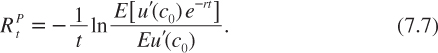
Following Weitzman (1998, 2001) and Gollier and Weitzman (2010), let us accept that there is unavoidable uncertainty over the rate of return of capital r when the investment decision must be made. It is assumed that r will be constant in the future, is uncertain this morning but will be known with certainty at the end of the day. To keep it simple, let us consider a numerical example in which r will be either 5% or 1% with equal probabilities. Thus, the opportunity cost of capital cannot be evaluated without error today. One dollar invested today in the productive capital of the economy will yield either exp(0.05t) or exp(0.01t) dollars at date t. So, it is hard to compare this benefit to the sure benefit F of the investment project. The NFV of this project is uncertain. One possible decision rule under uncertainty is to require that the sure cash flow of the project is larger than the expected cash flow of the investment in the productive capital of the economy, or alternatively that the expected NFV is positive. This is referred to as the expected NFV rule. It is equivalent to a rule which requires that the investment has an internal rate of return larger than a critical rate which is defined as follows:

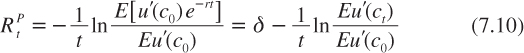
Weitzman (1998) provides an alternative decision rule under uncertainty which yields opposite results: A sure investment project should be implemented if its expected NPV is positive. In spite of the fact that this rule is equivalent to the expected NFV rule when there is no uncertainty (as was already explained), the decision rules are not equivalent when there is uncertainty. If the future benefit is offset by borrowing Fexp(–rt) once the rate r will be known, the net present benefit of the investment is equal to –1 + E [Fexp(–rt)], which is equivalent to discounting F at a rate defined as

As observed by Gollier (2004), using the positive expected NFV rule or the positive expected NPV rule leads to opposite results concerning the choice of the discount rate. In particular, it is obtained that

Moreover, the minimum and maximum bounds correspond to the asymptotic values of and respectively, when t tends to infinity. The NPV approach is more favorable to the evaluation of sure investment projects than the NFV approach, and this difference increases with the time horizon.

The analysis has also shown that the two rules differ by the date at which the risk associated with the alternative investment in the economy is allocated. Under the NFV approach, cash flows and risk are all transferred to the terminal date of the project, whereas they are all transferred to today under the NPV approach. This is a paradox, because of the huge difference in the practical consequences of the two approaches. In the spirit of the Modigliani–Miller’s Theorem, the evaluation of an investment project should not depend on the way that it is financed. In the absence of a clear description of the stakeholders’ preferences toward risk and time, it is not possible to determine which rule should be preferred, and which discount rate should be selected.

THE CASE OF THE LOGARITHMIC UTILITY FUNCTION

A surprising result of the expected NFV approach is that uncertainty affecting an investment project in the productive capital of the economy biases us to prefer this risky project against the sure one. This suggests that introducing risk aversion into the picture should make us favor the expected NPV rule which acts in the opposite direction.

Consistently, throughout this book, what matters for stakeholders is not the payoff of the project itself, but rather the utility that it generates. Before extending the analysis to a more general case, this section supposes that the utility function is logarithmic, u(c) = ln c. An important property of this function is that a change in the interest rate does not affect saving. The wealth effect perfectly compensates the substitution effect. This implies that at the end of the day, when r is observed, the level of consumption c₀ is insensitive to this information (this will be shown later in the chapter). However, consumption in the distant future will be highly sensitive to r. It can be shown that the optimal consumption at date t is proportional to exp(rt). Thus, at the beginning of the day, there is absolutely no uncertainty about the optimal consumption at the end of the day, but there is a huge uncertainty about consumption in the distant future.

Let us consider the expected NPV approach in this context. Remember that the NPV rule is based on the assumption that all cash flows from the sure marginal investment project are transformed into additional consumption at the end of the day, and only at that time. This additional consumption is uncertain (it depends upon the unknown r), but it is marginal. Because consumption c₀ at date 0 is risk-free, adding this marginal risk to initial wealth increases welfare if and only if the expected NPV is positive. Risk aversion is irrelevant. This is because (independent) risk is a second-order effect in the expected utility model (Segal and Spivak 1990). When introducing a small lottery into an initially risk-free situation, the first-order expectation effect always dominates. This can be seen from observing that, by the Arrow–Pratt approximation (3.3), the risk premium for small risk is proportional to the variance of the payoff, that is, to the square of the size of the risk. This means that the NPV formula (7.2) is perfectly valid when the representative agent has a logarithmic utility function.

What of the alternative expected NFV approach? This approach relies on the assumption that all the costs and benefits of the sure investment project are transferred to the terminal date t. Observe that the NFV is negatively related to the interest rate r, since the loan used to finance the initial cost of the project will yield a larger repayment at the terminal date when the interest rate is large. This means that the NFV of the sure project is negatively correlated with c_t. In other words, implementing the sure project by this financing strategy provides some hedging against the macroeconomic risk at date t. This is positively valued by consumers, something that equation (7.1) of the expected NFV approach fails to take into account. Therefore, this equation misprices the future.

To sum up, given a logarithmic utility function, when the sure investment project is implemented and cash flows are transferred to the present (the NPV approach), one can assume that the representative agent is risk neutral. This is because current consumption is risk-free. In contrast, taking the NFV approach, when the sure project is implemented and cash flows are transferred to the terminal date, this strategy serves as an insurance against wider macroeconomic risk. The risk neutrality assumption, implicit in equation (7.1), therefore cannot be sustained. Thus, when the representative agent has a logarithmic utility function, Weitzman’s formula (7.2) is right.

When the utility function of the representative agent is not logarithmic, the problem is more complex, because the optimal level of today’s consumption c₀ will react to changes in the rate of return of capital. Therefore, neither of the two rules (7.1) and (7.2) is valid. The next section is devoted to the analysis of this more general case.

TAKING ACCOUNT OF PREFERENCES TOWARD RISK AND TIME

When considering the expected NFV rule with risk aversion, the marginal additional consumption F – exp(rt) occurring at date t has a different marginal effect on utility in different future states of the world. This is because of the differing levels of consumption, c_t, that will be realized in these different states. The underlying strategy of financing the initial cost by a loan at rate r increases the expected utility at date t if

This is equivalent to using a discount rate follows:

This formula generalizes equation (7.1) to the case of risk aversion. Because c_t and r are likely to be correlated, the two equations are not equivalent. In fact, because GDP per capita is expected to be larger when the return on capital is larger, a negative correlation between u′(c_t) and r is expected. This implies that the numerator in equation (7.5) should be smaller than the product of Eu′(c_t) and Eexp(rt). In turn, this implies that the right-hand side of this equation should be smaller than the one in equation (7.1). Risk aversion should have a negative impact on the discount rate recommended under the expected NFV approach, and this effect is increasing with maturity. The intuition for this result is that investing in the productive capital of the economy yields a risk that has a positive correlation with wider macroeconomic risk which cannot be diversified. The associated risk premium of this strategy is increasing with the time horizon, favoring investment in the risk-free project.

The same method should also be used under the expected NPV approach. Remember that this approach is based on the assumption that the future cash flow of the risk-free project is offset by a loan of Fexp(–rt) at the end of the day. This strategy raises the expected utility of current consumption if

This is equivalent to using a discount ratedefined as

Under risk neutrality (u′ constant), this equation is equivalent to (7.2). The choice of consumption c₀ will in general depend upon the observation of the rate of return of capital at the end of the day. If the substitution effect dominates the wealth effect, c₀ and r are negatively correlated. This means that investing in the productive capital of the economy rather than in the safe investment project plays the role of insurance against low consumption in the short run. This reduces the relative attractiveness of the sure project under the expected NPV approach. This tends to raise the discount rate

TAKING ACCOUNT OF THE OPTIMALITY OF CONSUMPTION GROWTH

The introduction of risk aversion acts to reduce the gap between the two discount rates described by the inequalities in equation (7.3), by raising the lower rate and reducing the higher one. It is possible to go one step further by showing that the two approaches are in fact equivalent if it is assumed that consumers optimize their consumption plan contingent on their information about the future rate of return of capital. At the end of the day, r is realized, and consumers can decide how much to save or to borrow at that interest rate. Consider a marginal increase in saving at date 0 by 1 to finance an increase in consumption at date t by exp(rt). This marginal change in the consumption plan has no effect on welfare if

This is an optimality condition, which must hold for all possible realizations of r. This means that c₀ and c_t depend upon random variable r. If this condition is plugged into equation (7.7), it follows that:

Observe thus that = for all t! It can be concluded that once risk and risk aversion are properly combined with intertemporal optimization, the NPV and NFV approaches are equivalent. Moreover, these approaches are equivalent to the one on which the Ramsey rule and the previous chapters are based. Indeed, it also follows that:

The only difference with respect to what has been presented earlier in this book comes from the possibility that c₀ is random.

THE TERM STRUCTURE OF DISCOUNT RATES

In this model, in which shocks on capital productivity are permanent, risks affecting consumption growth are also permanent, as seen from equation (7.8). This implies that risk increases with maturity. This yields a decreasing term structure of discount rates. The property that the term structure must be decreasing can be proved by rewriting equation (7.9) as

where E^* is the standard risk-neutral expectation operator in which for any function F of r, we have E^*[F(r)] = E[u′(c₀(r))F(r)]/E[u′(c₀(r))]. Observe that the efficient term structure under this specification is equivalent to the Weitzman’s NPV formula (7.2) up to the risk-neutral transformation of the probability distribution. This implies that we get the same qualitative properties for the term structure as those generated by equation (7.2): it is decreasing and tends to the smallest possible rate of return of capital.

Let us examine this point in greater detail by characterizing the optimal allocation of risk and consumption through time. Suppose, as before, that relative risk aversion is a positive constant γ, so that u′(c) = c^-γ. One can solve equation (7.8) together with the intertemporal budget constraint

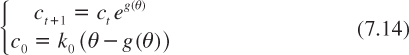
where k₀ is the initial level of capital per capita in the economy. A solution to this maximization program exists if r(1 – γ) < δ, which is true in particular when γ is greater than unity. The solution is written as

Observe first that the initial consumption c₀ is independent of the random variable r when γ equals unity. This confirms the property that initial consumption is not sensitive to the interest rate when the utility function is logarithmic (γ = 1). Observe also that, conditional on r, c_t has a constant growth rate g(r) = (r – δ)/γ. It is notable that this implies that the ex post equilibrium interest rate is r = δ + γg, which is the Ramsey rule. The problem is to determine the socially efficient discount rate before r is revealed. The fact is that ex post consumption will grow at a constant rate that is unknown ex ante. This simple model is thus equivalent to the following stochastic process for the growth of log consumption:

This is a special case of the general problem of parametric uncertainty that we examined in the previous chapter, but with an uncertain discrete jump in initial consumption. The arithmetic Brownian motion for log consumption is degenerate, with zero volatility, so that uncertainty is fully resolved at date 0. The riskiness of consumption increases exponentially through time, rather than linearly as in the case of log consumption following a Brownian motion.

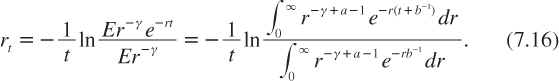
Following Weitzman (2010), let us calibrate this model by assuming that the uncertainty about the future rate of return of capital is governed by a gamma distribution:

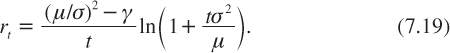
where a and b are two positive constants. This implies that the mean rate of return is Er = µ = ab and its variance is Var(r) = σ² = ab². Suppose that δ = 0 and γ > 1,¹ which implies from equation (7.13) that c₀ = K₀(γ-1)r/γ. The Ramsey pricing formula (7.10) can then be written as follows:

The two integrals in this expression have an analytical solution. Indeed, because the integral of the density f (r; k, h) must be equal to 1, we must have that

Suppose that γ < a. We can then apply this property twice in (7.16) for h = a – γ > 0 and respectively k = (t + b^-1)^-1 and k = b. It yields

It is easier to rewrite this equation with parameters (µ,σ) rather than (a, b). This substitution yields the risk-adjusted Weitzman’s formula

As long as γ is smaller than a = (µ/σ)², this term structure is decreasing, and tends to zero when t tends to infinity. Observe also that r₀ = µ–(γσ²/µ). Interestingly enough, an increase in risk aversion shifts the term structure downward in this model. This is because consumption c₀ is increasing in r, whereas the NPV is decreasing in r. This implies that investing in a safe project in this context provides a hedge for the immediate consumption risk. An increase in risk aversion makes safe projects more attractive. This is expressed by a smaller discount rate.

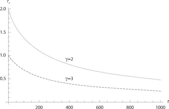
Figure 7.1. Discount rate with γ = 2 and 3 and with a gamma distribution for the permanent shock on the future return of capital. The mean future rate has a mean of 4% and a standard deviation of 2%.

Notice that equation (7.19) is equivalent to a hyperbolic discounting rule, since we have that

This is the functional form suggested by Loewenstein and Prelec (1991), to describe observed discounting behaviors. In figure 7.1, the discount rates are computed for a gamma distribution of the rate of return of capital with mean µ = 4% and standard deviation σ = 2%, together with γ = 2 and 3. Examine in particular the term structure for our benchmark calibration with γ = 2. Compared to the expected rate of return of capital of 4%, we see that the ex ante short-term efficient discount rate is only 2%. This illustrates the effect of risk aversion. The further reduction in the discount rate for longer maturities illustrates the growing precautionary effect.

The model proposed in this chapter is highly unrealistic because it makes the assumption that the uncertainty on the future return of productive capital will be completely revealed to us at the end of the day. This assumption on the permanency of the initial shock on interest rates is the driving force of the decreasing nature of discount rates. In reality, interest rates are subject to partially persistent shocks scattered through time. Newell and Pizer (2003), and Groom, Koundouri, Panopoulou, and Pantelidis (2007), have estimated the degree of permanency of shocks on interest rates, and have shown that it has a crucial role in the shape of the term structure of efficient discount rates.

SUMMARY OF MAIN RESULTS

1. Weitzman (1998, 2001, 2010) examines a model in which the exogeneous rate of return of capital is constant but random. Safe investment projects must be evaluated and implemented before this uncertainty can be fully revealed, i.e., before knowing the opportunity cost of capital.

2. A simple rule of thumb in this context would be to compute the net present value for each possible discount rate, and to implement the project if the expected NPV is positive. If the evaluator uses this approach, this is as if one would discount cash flows at a rate that is decreasing with maturity. This approach is implicitly based on the assumptions that the stakeholders are risk-neutral and transfer the net benefits of the project to an increase in immediate consumption. Opposite results prevail if one assumes that the net benefit is consumed at the maturity of the project.

3.  Fisher equivalence property: We have shown in this chapter that the evaluation of a sure (marginal) investment project is independent of how cash flows are allocated through time, as soon as it is recognized that economic agents are risk-averse and that they optimize their consumption plans.

4. Finally, once risk aversion and optimal consumption planning are introduced into the model, it has been shown that the term structure of discount rates should be decreasing in the context proposed by Weitzman. This is due to the increasing precautionary effect generated by the persistency of shocks in this economy.

REFERENCES

Gollier, C. (2004), Maximizing the expected net future value as an alternative strategy to gamma discounting, Finance Research Letters, 1, 85–89.

Gollier, C., and M. L. Weitzman (2010), How should the distant future be discounted when discount rates are uncertain? Economic Letters, 107 (3), 350–353.

Groom, B., P. Koundouri, E. Panopoulou, and T. Pantelidis (2007), An econometric approach to estimating long-run discount rates, Journal of Applied Econometrics, 22, 641–656.

Loewenstein, G., and D. Prelec (1991), Negative time preference, American Economic Review, 81, 347–352.

Newell, R., and W. Pizer (2003), Discounting the benefits of climate change mitigation: how much do uncertain rates increase valuations? Journal of Environmental Economics and Management, 46 (1), 52–71.

Segal, U., and A. Spivak (1990), First order versus second order risk aversion, Journal of Economic Theory, 51, 111–125.

Weitzman, M. L. (1998), Why the far-distant future should be discounted at its lowest possible rate? Journal of Environmental Economics and Management, 36, 201–208.

Weitzman, M. L. (2001), Gamma discounting, American Economic Review, 91, 260–271.

Weitzman, M. L. (2010), Risk-adjusted gamma discounting, Journal of Environmental Economics and Management, 60, 1–13.

¹ There is a discountinuity of the term structure with respect to γ at γ = 1. A similar analysis to the one presented in the text yields r_t = (µ²/tσ²) ln (1+(tσ²/µ)).