3

Extending the Ramsey Rule to an Uncertain Economic Growth

It is commonly accepted that individuals are ready to sacrifice more in the present for the future when this future becomes more uncertain. Keynes was the first to mention this idea by pointing out the precautionary motive for saving. What is desirable at the individual level is also desirable at the collective one. A society that wants to reinforce the incentive to invest for the future because of its uncertain nature should select a smaller discount rate to evaluate the set of all possible investment projects. We formalize these ideas in this chapter.

A DECISION CRITERION UNDER RISK

Uncertainty is a feature of everyday life. We don’t know with certainty today what tomorrow will look like, and for many of us, the more distant future is extremely uncertain. This complicates the dynamic optimization problem of maximizing our lifetime welfare together with the valuation of our investment projects. In particular, determining the optimal level of savings requires an estimate of the future utility gain of this transfer of wealth in a context in which little is known about future incomes. This problem is at the core of the question of what should be done for the future.

When the growth rate of consumption is unknown, the intensity of the wealth effect described in the previous chapter cannot be estimated, and the Ramsey rule (2.12) is unable to produce a precise prescription for the choice of the discount rate. Estimating the growth rate of consumption for the coming year is already a difficult task. Any estimate of growth for the next decade is subject to potentially very large errors. Over a century, estimation errors could be enormous.

The history of the western world before the industrial revolution is full of significant economic slumps, such as those that occurred following the collapse of the Roman Empire in the fifth century, or the Black Death epidemic in the mid-fourteenth century. The recent debate on the concept of sustainable growth is itself an illustration of the degree of uncertainty faced when thinking about the future of society. Some argue that the effects of improvements in information technology have yet to be realized and that the world is entering a period of more rapid growth. By contrast, those who emphasize the effects of natural resource scarcity, or the inability of financial markets to allocate capital efficiently, predict lower growth rates in the future. Some even suggest a negative growth of GDP per head, owing to a deterioration of the environment, population growth, and decreasing returns to scale. The implication of this last position is that the wealth effect on the discount rate is negative rather than positive as supposed in the previous chapter. Under these plausible beliefs, the future is poorer than the present so we should make more sacrifices today to improve the future. We are unable to tell which scenario is right, and which is wrong, in other words, our future is uncertain by nature. Uncertainty over how wealthy the future will be at least casts some doubt on the relevance of the wealth effect to justify the use of a large discount rate.

In order to address the question of the role of uncertainty on the selection of the discount rate, it is necessary to characterize its impact on welfare. From now on the classical approach is followed, relying on the Bernoulli–von Neumann–Morgenstern expected utility theory. More specifically, it is assumed that when the consumption level c_t at date t is uncertain, the ex ante welfare at that date is measured by the expected utility of this uncertain consumption. Thus, seen from date 0, the social welfare in the economy is written as

where the expectation operator E is related to the probability distribution of the random variable c_t. The expected utility criterion relies on an intuitive “independence axiom.” Consider three different actions, A, B, and C. A could be to go to see a movie; B could be to go to a restaurant, and C to stay home. Under the independence axiom, if one prefers A with certainty rather than B with certainty, one will also prefer the lottery which yields A with probability p to the lottery which yields B with the same probability, where for both lotteries the alternative is to get C with probability 1 – p. In other words, if you prefer to go to the movie rather than the restaurant today, this choice will not be altered if you learn that there is a risk that you will have to stay home with some probability p. In spite of its intuitive appeal, the Allais’ paradox (Allais 1953) shows that there are circumstances under which some agents violate this axiom. However, the aim of this book is mostly normative. An answer is sought to the question of which discount rate should be used for rational evaluation of public policies. For this purpose, it is reasonable to rely on the very intuitive and normatively appealing independence axiom.

RISK AVERSION

An agent is risk-averse if he always prefers the expected payoff of a lottery to the lottery itself. In the expected utility model, it is well-known that the concavity of the von Neumann–Morgenstern utility function characterizes the aversion to risk of the decision maker. Indeed, by Jensen’s inequality, the concavity of u implies that Eu(c_t) is smaller than u(Ec_t). A mean-preserving reduction in risk increases expected utility because marginal utility is decreasing. For example, if future consumption is 80 or 120 with equal probabilities, decreasing marginal utility implies that increasing consumption by 20 in the bad state increases utility more than the reduction of utility from reducing consumption by 20 in the good state. Therefore, eliminating the risk and receiving 100 with certainty is ex ante welfare-improving.

Let z = Ec_t and ε_t = (c_t – Ec_t)/Ec_t denote respectively the expected consumption and the relative risk at date t. In addition, let π denote the risk premium, which is defined as the maximum price that one is ready to pay for the full elimination of ε_t, expressed as a fraction of expected consumption:

The level of π measures the degree of aversion to relative risk ε. Case π = 0 corresponds to risk neutrality, in the sense that risk does not affect welfare in that case. The well-known Arrow–Pratt approximation allows us to link π to the variance of ε_t and to the index of the concavity of u, which is R(c) = –cu″(c)/u′(c)

The relative risk premium is approximately equal to half the product of the variance of the relative risk and of the index of relative risk aversion R. This is obtained through Taylor approximations of the two sides of equation (3.2) around z.

Equation (3.3) gives us a new opportunity to estimate the degree of concavity of u. Suppose that your consumption is subject to an equal chance of an increase or a decrease of 10%. What fraction of consumption are you prepared to pay to eliminate this risk? Since equals 1% in this case, the answer to this question should approximately be equal to 0.5% of R. For example, when relative risk aversion equals 2, this fifty-fifty chance of a gain or a loss of 10% of consumption is equivalent to a sure loss of π 1%. This test provides further reassurance that R = 2 is a reasonable level of concavity of the utility function.

How good is the Arrow–Pratt approximation (3.3)? In general, because it is derived from Taylor approximations, its quality decreases as the size of risk ε_t increases. There is however one special case in which approximation (3.3) is exact, whatever the size of the risk. This special case is used almost universally in the theory of finance, and is applied extensively later in this book. For these reasons it is good to write it as a formal lemma.

Lemma 1: Suppose that x is normally distributed with finite mean μ and variance σ². Consider any scalar A ∈ . Then:

In other words, the Arrow–Pratt approximation (3.3) is exact when the risk is normally distributed and the utility function is exponential.

A proof of the first part of lemma 1 is provided in the appendix of this chapter. Using (3.4), it is immediate that approximation (3.3) is exact when u(c) = –e^–Ac and ε is normally distributed with mean 0 and variance σ². The reader will check that R(z) = Az in this case.

It is notable that in the additive model (3.1), which is also referred to as the “Discounted Expected Utility” model, the concavity of u plays two different roles: aversion to intertemporal inequality and aversion to risk. This has often been criticized in the literature because the attitudes toward risk and time are often considered to have different natures. This limits the positive power of the model, to describe how people behave in relation to risk and time. However, from a normative point of view, the use of decreasing marginal utility to explain the two types of aversion is quite appealing. It makes sense to link the resistance to transfer wealth either to a wealthier future or to a wealthier state of nature to the property that marginal utility is decreasing.

PRUDENCE AND PRECAUTIONARY SAVING

The previous section examined the impact of risk on welfare. However, the main question here is quite different. We are interested in determining the impact of uncertainty on willingness to improve the future. Before examining this question at a global level, it is useful to return to the individual level. The most obvious action that we take in favor of our own future is to save. So, it is useful to explore the effect on saving behavior of uncertainty over future income. This provides a helpful insight into how we should collectively behave in the face of an uncertain collective destiny. After all, any collective risk will percolate down into risks that must be borne by individuals. Intuition suggests that uncertainty surrounding the future should raise our willingness to save. This is the concept of precautionary saving introduced by Keynes, which has been revisited since then by Leland (1968), Drèze and Modigliani (1972), and Kimball (1990), among others.

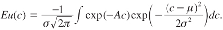
Consider individuals who have a flow of income y₀ at date 0, and y_t at date t. Their optimal level of saving, s, solves the following maximization program:

where r is the interest rate. Under the concavity of u, the objective function V is concave in s, and the following first-order condition is necessary and sufficient:

Compare two cases. In the certainty case, y_t equals a constant z with certainty. Without loss of generality, suppose that the optimal saving level is zero in that case. This is true if

In the uncertainty case, y_t = z(1 + ε_t), where ε_t is a zero-mean relative risk on future income. Compared to the certainty case, the future risk raises the optimal saving if and only if it raises V′(0). This requires that:

Using condition (3.7), this is equivalent to

This is the case for all z and for all zero-mean ε_t if and only if u′ is convex. In words, marginal utility must be decreasing at a decreasing rate to guarantee that precautionary saving is nonnegative. Using the terminology introduced by Kimball (1990), an agent is called prudent if his marginal utility is convex. Prudence is the necessary and sufficient condition to guarantee that individuals want to save more when the future becomes more uncertain.

Let us define the precautionary premium ψ as the sure relative reduction in future income that has the same effect on saving as the future risk on income:

We say that (1 – ψ)Ec_t is the precautionary equivalent of c_t = (1 + ε_t)Ec_t. Comparing equations (3.10) and (3.2), observe that the precautionary premium ψ of u is the risk premium of –u′, which is increasing and concave under prudence. By analogy, equation (3.3) can be rewritten as:

where P(z) = –zu′″(z)/u″(z) is the index of relative prudence (Kimball 1990). Thus, adding a zero-mean relative risk to future consumption has an effect on current saving that is approximately equal to half the product of the variance of this risk and of the index of relative prudence.

There has not been much attempt to estimate individuals’ degree of prudence. Usually, researchers use one of a family of utility functions that require the choice of a single parameter which determines both the degree of risk aversion of the decision maker and their degree of relative prudence. In practice, the choice of this parameter is calibrated to the assumed degree of risk aversion. For example, consider the case of the power utility function, with u′(c) = c^–γ, which implies that u″(c) = –γc^–γ–1<0 and u′″(c) = γ(γ + 1)c^–γ–2 > 0. It yields R(c) = γ and P(c) = γ+1. For power functions, relative prudence equals relative risk aversion plus one. If we take R = 2, we obtain P = 3. Facing an equal chance of gaining or losing 10% of future income has an effect on current saving that is approximately equivalent to the effect of a sure reduction of future income by 1.5%.

PRUDENCE AND DOWNSIDE RISK AVERSION

Is the convexity of marginal utility a natural assumption to make? It has already been assumed that marginal utility is positive and decreasing. This implies that it must be convex, at least locally, for large consumption levels. Observe also, though this is not a very convincing argument, that all classical utility functions used in economics exhibit a convex marginal utility. This is the case for exponential, power, and logarithmic utility functions. The quadratic utility function has a linear marginal utility.

Two positive arguments are in favor of prudence. The first is that there is empirical evidence that people increase their saving when their future becomes more uncertain. See for example the econometric analysis by Guiso, Jappelli, and Terlizzese (1996). Second, people are downside risk-averse, which is another term for prudence. The meaning of downside risk aversion can be illustrated by the definition proposed by Eeckhoudt and Schlesinger (2006). Suppose that your future consumption is either a low z_l or a high z_h, with equal probabilities. Suppose that you are forced to bear a zero-mean risk in one of these two states. Do you prefer to allocate this risk to the low- or high-consumption state? If you answer that it is better to face the risk in the high-consumption state then you are downside risk-averse. This is true if and only if

or equivalently:

Rewriting this inequality:

Because z_l and z_h > z_l are arbitrary, this integral is positive if and only if Eu′(z + ε) ≥ u′(z) for all z. It follows that the preference for putting risk in the higher income state requires that marginal utility is convex. Prudence and downside risk aversion are two equivalent concepts.

THE EXTENDED RAMSEY RULE AS AN APPROXIMATION

Uncertainty surrounding the growth of consumption affects the discount rate. Let us consider a marginal investment that has a unit cost today and that yields a sure benefit R = exp(rt) at date t. It preserves the intertemporal welfare V defined by (3.1) if and only if:

This can be rewritten:

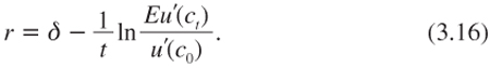
Now, remember that the existence of the relative risk ε_t = (c_t – Ec_t)/Ec_t on future consumption has an effect on expected marginal utility that is equivalent to a sure relative reduction of consumption by the precautionary premium. Technically, using (3.10), equation (3.16) can be rewritten as:

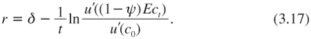
This is a return to the certainty case that was examined in the previous chapter. For example, approximation (2.11) can be rewritten as follows:

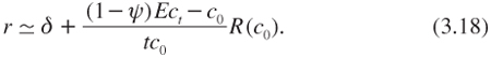
This is reminiscent of the Ramsey rule with an impatience effect and the wealth effect, but the latter is reduced by risk. This reduction ψ can be approximated by using equation (3.11). Alternatively, a second-degree Taylor approximation of u′(c_t) around c₀ can be used in equation (3.16) to get:

This is the extended Ramsey rule. As in the standard Ramsey rule (2.11), there is an impatience effect and a wealth effect. The third term in the right-hand side of (3.19) is what is called the precautionary effect. It tends to reduce the discount rate. Its intensity is proportional to the product of relative prudence, relative risk aversion, and the annualized variance of the growth rate of consumption between 0 and t.

This confirms the intuition that uncertainty affecting the future tends to raise our willingness to invest for that future. Uncertainty over future economic growth translates into a lower discount rate, lowering the threshold rate of return that a sure investment must achieve to be considered welfare enhancing.

THE EXTENDED RAMSEY RULE IN THE LOGNORMAL CASE

The extended Ramsey rule described by (3.19) can be obtained as an exact solution in an important special case. Let us consider a one-year horizon (t = 1). Suppose that

where x is the continuously compounded growth rate of consumption, or the increase in the logarithm of consumption. Let us assume that x is normally distributed with mean μ and variance σ². Notice that, using lemma 1 and equation (3.4) with A = –1, implies that the growth rate of expected consumption (or the change in log expected consumption) between dates 0 and 1 is g = 1n(Ec₁/c₀) = Ee^x = μ + 0.5σ²

Suppose also that the representative agent in the economy has a power utility function, with u′(c) = c^–γ. This implies that

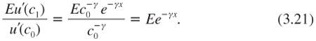
Now, equation (3.4) can be used again to rewrite the right-hand side of equation (3.21) as exp(–γ(μ – 0.5γσ²)). Plugging this into the pricing formula (3.16) yields

It is preferable to rewrite this formula using the growth rate g of expected consumption:

This exact extended Ramsey rule combines the three components of the efficient discount rate: impatience, the wealth effect, and the precautionary effect. As in the Ramsey rule under certainty, the wealth effect is positive and is the product of the expected growth rate of consumption by the relative aversion to intertemporal inequality. The precautionary effect is negative, and is equal in absolute value to half the product of three factors: relative risk aversion γ, relative prudence γ + 1, and the variance of the growth rate of consumption. This shows that approximation (3.19) is exact in the special case of a power utility function and a log normal distribution of future consumption.

CALIBRATION OF THE EXTENDED RAMSEY RULE USING TIME SERIES DATA

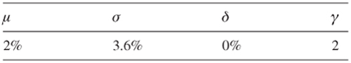
In the previous chapter, in which risk was ignored, a justification was provided for the use of δ = 0, γ = 2, and g = 2%. In turn, this justified using a discount rate of 4% per year. How much smaller than 4% should the discount rate be to take account of future risk? To answer this question for a one-year horizon, the volatility of the annual growth rate of consumption must be estimated.

Kocherlakota (1996), using U.S. annual data over the period 1889–1978, estimated the standard deviation σ of the growth of consumption per capita to be 3.6% per year. Assuming normality and an expected growth rate of 2%, this means that there is a 95% probability that the actual growth rate of consumption next year will be between –5% and +9%. Using σ² = (0.036)² and γ = 2 as stated in table 3.1 yields a precautionary term in the extended Ramsey rule (3.23) equaling –0.4%. The precautionary effect reduces the efficient rate at which one should discount cash flows occurring next year from 4% to 3.6%.

TABLE 3.1.
Benchmark calibration of the extended Ramsey rule

In Gollier (2011), we have calibrated the extended Ramsey rule for other countries. In this exercise, whose results are described in table 3.2, it is assumed that each country has its own stable trend and volatility for the growth rate of its economy. In order to estimate them, we used a data set of real historical GDP per capita extracted from the Economic Research Service (ERS) International Macroeconomic Data Set provided by the U.S. Department of Agriculture (USDA). This set contains the real GDP/cap expressed in dollars of 2005 for 190 countries for each year from 1969 to 2010. If we limit the analysis to the United States, the first two moments of the growth rate of GDP/cap over the period has been respectively g = 1.74% and σ = 2.11%. With δ = 0% and γ = 2, it yields a wealth effect of 3.48% and a precautionary effect of –0.13%, implying a discount rate of 3.35%.

We obtain the same order of magnitude for the wealth effect and the precautionary effect for other developed countries like France, Germany, and the United Kingdom. For Japan, the mean growth rate and the volatility have been larger, yielding a net positive effect with a discount rate around 4.5%. The picture is quite different for emerging countries, which by definition experienced a much larger growth rate of consumption. The most striking example is China, with a mean annual growth rate of around 7.5% per year, and a relatively large volatility around 4%. The calibration of the extended Ramsey rule (3.23) with these parameter values yields a discount rate as large as 14.82%. If one believes that this growth is sustainable, intertemporal inequality aversion and the associated wealth effect should induce the Chinese authorities to limit their safe investments to projects having a rate of return above this large discount rate.

TABLE 3.2.
Country-specific discount rate computed from the extended Ramsey rule using the historical mean g and standard deviation σ of growth rates of real GDP/cap 1969–2010

At the other extreme of the spectrum is the set of countries that have experienced low growth rates. The worst example is Zaire (RDC), with an awful mean growth rate of –2.76% per year over the last four decades. If one believes that this negative growth trend is persistent, a negative discount rate of –6.38% should be used to evaluate safe projects in that country. Liberia provides another example of a country with a negative discount rate. In this country, the volatility of the growth rate has been extremely large, with s equaling 19.58%. This implies a precautionary effect around –11.5%. Combining that with a wealth effect of –3.8%, we obtain a socially efficient discount rate for Liberia around –15%. These examples clearly show the shortcomings of this calibration exercise. In particular, it is implicitly assumed here that the future will look like the past, and that there is no business cycle. For Sub-Saharan countries, we hope that the future will not look like the past.

The important differences in growth outcomes among the 190 countries present in the ERS/USDA data set over the last four decades make it difficult to draw general conclusions about the discount rate. In table 3.3, we summarize the calibration of the extended Ramsey rule on the basis of the mean wealth and precautionary effects among the 190 countries of the data set.

In figure 3.1, we draw the frequency graph for the wealth effect and the discount rate. It is noteworthy that the precautionary effect tends to be much smaller in developed countries, because of the more efficient stabilizing policies put in place in these countries. This is an important reason for the relatively larger discount rates that are efficient in the western world. Precautionary investment is a substitute to macroeconomic stabilizing policies.

TABLE 3.3.
The mean discount rate among the time series of the 190 countries

Mean wealth effect	3.54% per year
Mean precautionary effect	–1.00% per year
Mean discount rate	2.54% per year

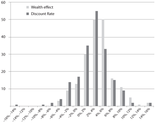
Figure 3.1. Frequency for the wealth effect and the discount rate among the 190 countries, using the extended Ramsey rule

This exercise in which we apply the extended Ramsey rule (3.23) to each individual country relies on the assumption that risks are efficiently shared within each country, so that the volatility of the growth of GDP/cap is the right measure of uncertainty born by all citizens within that country. By the power of imagination, suppose that risks are efficiently shared at the level of the entire world, so that the growth of world GDP/cap would be the right measure of consumption growth of all human beings on the earth. Expectations about the future can be inferred from the first two moments of the growth of world GDP/cap over the last four decades. Using the same data set, we obtain by pure chance that the mean and the volatility of the real growth rate of world GDP/cap are equal to 1.41%. This yields a wealth effect and a precautionary effect of respectively 2.82% and –0.06%, implying a discount rate of 2.76%. Because country-specific risks are washed out through international diversification, the small precautionary effect reflects the low systematic risk at the aggregate level. However, this exercise has no economic meaning because it is clear that credit and risk-sharing markets do not work efficiently at the international level. Even in an integrated economic union like Europe, there is little international solidarity across borders.

To sum up our results in this section based on a time-series analysis of country-specific economic growth, one must admit that the precautionary effect remains a marginal component in the estimation of the socially efficient discount rate. For the western world, the precautionary effect is generally smaller than a quarter of a percent, and is close to 0.1% for countries like the United States, France, the United Kingdom, and Germany. This is because of the low volatility of their economic growth observed during the last four decades. This precautionary effect is marginal compared to the usually much larger wealth effect equaling two times the anticipated growth rate. However, this conclusion of the limited role of uncertainty to determine the intensity of our sacrifices in favor of the future does not hold for developing countries. Many of them have experienced a huge volatility of their growth rate during the same period. This suggests that the discount rate that should be used in these countries should be smaller than in the western world, even in the case of similar expectations on the trend of economic growth.

CALIBRATION OF THE EXTENDED RAMSEY RULE USING CROSS-SECTION DATA

In the previous section, we made the assumption that each country faces its own stochastic growth process characterized by a random walk for the annual growth rate of consumption with known country-specific mean and volatility. If we take a more long-term perspective, one must recognize that growth processes undergo persistent shocks, or that they are subject to long-lasting cycles covering several decades. Contrary to what is implicitly assumed in the previous computations, it is indeed hard to believe that China will be able to stay permanently with a trend of growth around 8% per year, or that Zaire will permanently face an expected growth rate of –2.7% per year. Based on this idea, Gollier (2011) proposes consideration of an alternative modeling of growth risk other than the one that is classically considered in the literature, as illustrated in the previous section. In the spirit of Kondratiev waves ranging from forty to sixty years in length, let us consider the abstract stochastic growth process in which each country-specific growth rate is reset every forty-one years with resetting dates 1969, 2010, 2051, … To be more precise, let us assume that each country-specific change in log consumption x₄₁ is drawn from the same worldwide “urn” which is normally distributed with mean μ = g – 0.5σ² and volatility σ. This allows us to again use equation (3.23) to estimate the socially efficient rate r at which cash flows occurring in forty-one years should be discounted at each resetting date. In this framework, all countries should use the same discount rate ex ante.

The observation of the change in log consumption between 1969 and 2010 in the 190 countries of the ERS/USDA data set allows us to estimate the first two moments of random variable x₄₁. Its mean and its volatility are respectively equal to μ = 65.74% and σ = 72.18%. It yields a growth rate of expected consumption equaling g = μ + 0.5σ² = 91.79%, or 2.24% per year. The calibration of the extended Ramsey rule in this cross-sectional analysis is summarized in table 3.4.

Focusing on the annualized rates, two conclusions should be drawn from these results when tables 3.3 and 3.4 are compared. First, the relatively large growth rate of expected consumption in this model implies a large wealth effect in the Ramsey rule. But the precautionary effect is also large, amounting to almost 4% per year. Remember that the mean level of the precautionary effect that we documented in the previous section was only 1%. This huge difference in the precautionary effect when using a cross-sectional approach rather than the traditional time-series approach comes from the important heterogeneity in the country-specific growth rates observed during the last four decades. In other words, there is more volatility across countries than through time. The bottom line is a small discount rate at 0.67% per year.

TABLE 3.4.
The discount rate using the cross-section approach during period 1969–2010

Wealth effect	183.59%	4.48% per year
Precautionary effect	–156.30%	–3.81% per year
Discount rate	27.29%	0.67% per year

SUMMARY OF MAIN RESULTS

1.  Under prudence (u″′ ≥0), uncertainty about the growth of aggregate consumption induces people to invest more for the future. At the collective level, this is done by reducing the discount rate.

2.  Quantitatively, the precautionary effect reduces the discount rate by half the product of three factors: relative risk aversion, relative prudence, and the variance of the growth rate of consumption. Under CRRA, this is equal to 0.5γ(γ + 1)σ².

3.  The volatility of the growth rate of the US GDP/cap over the last century is around 3.6%. It justifies reducing the short-term discount rate by 0.4%. In short, taking account of short-term risk, the efficient short-term discount rate should be reduced from 4% to 3.6%.

4.  Examining other developed countries and other time periods does not radically transform the message that uncertainty does not have a strong impact on short-term discounting.

In the second part of this book, the question of uncertainty is explored further, by considering risk in the longer term and its implications for discount rates.

APPENDIX

Lemma: Suppose that x is normally distributed with finite mean μ and variance σ². Consider any scalar A ∈ . Then, we have that

Proof: Suppose that u(c) = –exp(–Ac). If c is normally distributed with mean μ and variance σ², we have that:

Rearranging the integrant, we obtain:

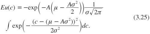
Observe that:

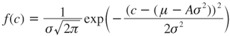
is the density function of a normally distributed random variable c with mean μ–Aσ² and variance σ². Because the integral of a density function equals 1, this implies that we can rewrite (3.25) as follows:

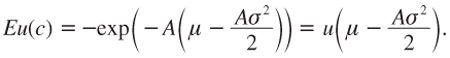
This concludes the proof of the lemma.

REFERENCES

Allais, M. (1953), Le comportement de l’homme rationnel devant le risque, Critique des postulats et axiomes de l’école américaine, Econometrica, 21, 503–546.

Drèze, J. H., and F. Modigliani (1972), Consumption decisions under uncertainty, Journal of Economic Theory, 5, 308–335.

Eeckhoudt, L., and H. Schlesinger (2006), Putting risk in its proper place, American Economic Review, 96 (1), 280–289.

Gollier, C. (2011), On the underestimation of the precautionary effect in discounting, Geneva Risk and Insurance Review, 36, 95–111.

Guiso, L., T. Jappelli, and D. Terlizzese (1996), Income risk, borrowing constraints, and portfolio choice, American Economic Review, 86, 158–172.

Kimball, M. S. (1990), Precautionary saving in the small and in the large, Econometrica, 58 (1990), 53–73.

Kocherlakota, N. R. (1996), The equity premium: it’s still a puzzle, Journal of Economic Literature, 34, 42–71.

Leland, H. E. (1968), Saving and uncertainty: The precautionary demand for saving, Quarterly Journal of Economics, 465–473.