14

Evaluation of Non-marginal Projects

The beauty and usefulness of cost-benefit analysis is that it relies on a few numbers, which represent the social value of the different dimensions of costs and benefits: the value of life, the value of environmental assets, the discount rate, or the risk premium for example. Once these values are determined, the evaluator is just required to estimate the flows of these multi-dimensional impacts, and to value them according to these prices. We show in this chapter that this simple toolbox can be used only if the actions under scrutiny are marginal, that is, if implementing them has no macroeconomic effects. Otherwise, one needs to go back to the basics of public economics to evaluate these actions. Alternative non-marginal strategies need to be compared through their impact on the social welfare function, whose description may raise new questions and new challenges in the public debate.

In this book we used the classical marginalist approach to value investments and assets. Under this approach, prices and values express marginal rates of intertemporal substitution. We obtained the ubiquitous pricing formula for the discount rate by considering a marginal transfer of consumption through time. For the risk premium, we evaluated a marginal introduction of the investment risk on welfare. This approach makes sense to express prices that sustain equilibrium with divisible goods, but this requires knowing the allocation at equilibrium. This approach also makes sense when one normatively evaluates a marginal action along the current equilibrium consumption path. It does not make sense when one evaluates non-marginal projects. Non-marginal projects are those which have an impact on the consumption path, so that they affect equilibrium prices and normative values. Discount rates and risk premiums become endogenous in that case.

Following Gollier (2011), let us illustrate this point with two examples. The first one is provided by Dietz and Hepburn (2010), and is about a large infrastructure project in Laos. The Nam Theun II hydropower dam project has a generation capacity of 1 giga-watt from a 350 meter-difference in elevation between the reservoir and the power station. The construction cost was US$ 1.3 billion, to be compared to gross consumption of the country, which is around US$2.5 billion. The construction started in 2005, and was completed in the spring of 2010. The export of electricity is expected to yield an annual benefit of US$250 million. From these figures, it is clear that the implementation of the project does affect the growth rate of the economy, and the willingness to invest for the future. Therefore, the choice of the discount rate to evaluate the project and to optimize its size must be endogenously determined.

The second example is in the context of climate change. In Dietz, Hope, and Patmore (2007), the expected damages due to climate change in the business-as-usual “high-climate” scenario are evaluated to 13.8% of world GWP in 2200. The 5–95% confidence interval spans a range from 2.9% to 35.2% of GWP. Consider a strategy that would eliminate these damages at some non-marginal cost. If we use the classical approach of discounting, should we use the extended Ramsey rule with a reduced growth rate to take into account the increasing damages, and with an increased uncertainty on growth coming from the uncertainty about these damages? This is problematic if the aim of the policy is precisely to reduce the intensity and the uncertainty of climate change!

When comparing different non-marginal policies, one needs to go back to the basic principles of public economics. If option A yields a consumption path and if option B yields a consumption path , option A dominates option B if and only if it yields a larger discounted expected utility:

This approach is rarely used in cost-benefit analyses, probably because of the complexity of the problem. Indeed, it requires a full description of the utility function, of the rate of pure preference for the present, and of the joint probability distribution of the status-quo consumption and of the payoff of the action. In spite of these challenges, this approach to the evaluation of non-marginal projects was undertaken by Nordhaus and Boyer (2000), Stern (2007), and Nordhaus (2008). Tol (2005), who reviewed the empirical literature on the estimation of the shadow value of emission abatement, showed that 62 of the 103 estimations of shadow value of carbon ignored the non-marginal nature of the impacts of climate change and of our global strategy to limit them.

Following Dietz and Hepburn (2010), we hereafter examine the error that one makes by following the classical discounting approach when evaluating non-marginal projects.

EVALUATION ERROR FOR THE DISCOUNT RATE

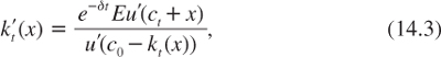
Suppose that we use the classical discounting approach to evaluate a project that has a non-marginal impact on the growth of consumption. What is the sign and the size of the error that one makes on the true value of the project? Concerning the sign of the effect, the intuition is quite simple. If the project is standard, with a cost incurred today for a sure benefit in the future, investing in the project will raise the expected growth rate of consumption. It will increase the discount rate through the wealth effect. Thus, the classical discounting approach will rely on a too small discount rate. Therefore, since it underestimates the discount rate, it overestimates the social value of the project. Consider a project that reduces current consumption by k today, and that increases consumption by a sure amount x at some specific date t. What is the maximum cost k that one is ready to incur today to get x at date t? In other words, what is the present value of increasing consumption by x at date t? Earlier in this book, we addressed this question in the special case with x being small, and we obtained that , where r_t is the discount rate. Suppose now that x is not small. The maximum cost that one is ready to incur today to get x at date t is a function k_t (x) whose properties are explored in this section. This function is defined as follows:

where c₀ and c_t are consumption levels in the status-quo scenario respectively at dates 0 and t. If the maximum cost is incurred, investing has no effect on the intertemporal utility of the agent. This means that k_t (x) is the value of x. Our aim here is to compare . Of course, we have that k(0) = 0. What about k′(0)?

Differentiating equation (14.2) with respect to x yields

which is positive. Using pricing formula (4.1) yields

Not surprisingly, this result just states that the linear extrapolation k_t(x) is exact for marginal projects. Differentiating once again, equation (14.3) yields in turn

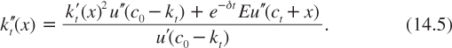
This is unambiguously uniformly negative. Thus, the valuation function k_t(x) is increasing and concave. It implies that the extrapolation formula which is systematically used in cost-benefit analyses overestimates the true social value of all projects with positive future cash flows.

One can estimate the order of magnitude of the valuation error by considering the following numerical example. Normalize current consumption to unity. Suppose that the growth rate of consumption is a safe 2%, that relative risk aversion is a constant equaling 2, and that the rate of impatience is zero. In this framework, the discount rate is 4%. The true present valuation function k_t (x) is depicted in figure 14.1 for a project with a one-year time horizon (t = 1). It appears that it is very quickly different from xe^–0.04. For example, for a benefit that represents 10% of current consumption, the true present value is k_t (0.1) = 8%, which should be compared to the traditional valuation 0.1e^–0.04 = 9.6%. The (over-)estimation error represents one-fifth of the true present value.

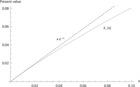
Figure 14.1. The true present valuation function as a function of the size x of the future benefit. We assume that t = 1, c₀ = 1, c₁ = 1.02, δ = 0, and u′(c) = c^–2. The dashed line corresponds to the present value extrapolated from the Ramsey rule (r = 4%).

THE SIZE-ADJUSTED EFFICIENT DISCOUNT RATE

The use of an explicit welfare function to evaluate a non-marginal project may be cumbersome for practioners. We hereafter elaborate an alternative approach in which we preserve the basic discounting approach, but in which we adapt the discount rate to take into account the size of the project. This may be done by defining the size-adjusted discount rate r_t (x) by the following condition:

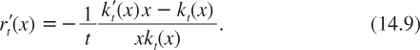
where k_t (x) is defined by condition (14.2). If the cost of the project is less (larger) than its present value defined by (14.6), its implementation will obviously raise (reduce) the intertemporal welfare, so that r_t (x) can indeed be interpreted as a size-adjusted discount rate. It can be rewritten explicitly as

Using L’Hospital’s rule, we obtain the standard formula for marginal projects:

where the second equality is obtained from (14.3). We are interested in measuring the sensitivity of the discount rate in the neighborhood of small benefits. By condition (14.7), we have that

Using L’Hospital’s rule twice, we obtain:

From equations (14.4) and (14.5), we have that

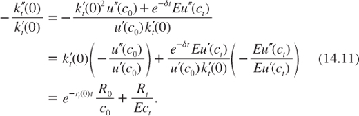
where R₀ = –c₀u″(c₀)/u′(c₀) is the index of relative risk aversion evaluated at c₀, and R = –Ec_tEu″(c_t)/Eu′(c_t) is the risk-adjusted relative risk aversion at date t. Combining equations (14.10) and (14.11) yields

where is the annualized growth rate of expected consumption between dates 0 and t. Notice that the left-hand side of equation (14.12) is the quasi-elasticity of the discount rate relative to the size of the cash flow in the neighborhood of x = 0. It measures the percentage increase in the efficient discount rate when the cash flow at date t increases by 1% of expected consumption. When t is normalized to unity, the right-hand side of this equality is close to the average of relative risk aversion evaluated at dates 0 and t.

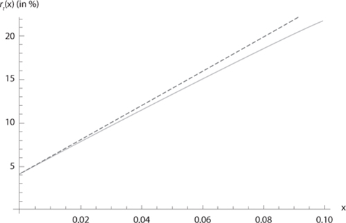
Figure 14.2. The size-adjusted discount rate as a function of the size x of the future benefit. We assume that t = 1, c₀ = 1, c₁ = 1.02, δ = 0, and u′(c) = c^-2. The dashed line corresponds to size-adjusted rate from the first-order Taylor approximation

Let us reconsider the numerical example of the previous section, with t = 1, c₀ = 1, c₁ = 1.02, δ = 0, and u′(c) = c^–2. It yields R₀ = R₁ = 2 and Exp (μ₁–r₁(0)) = 0.98. Consider a benefit that represents 1% of consumption at date 1. Adjusting for the size of this benefit would require increasing the discount rate from 4% to 4% + 1% × (0.98 × 2 + 2)/2 = 5.98%. In figure 14.2, we draw function r_t (x) for benefits x up to 10% of future GDP.

EVALUATION ERROR FOR THE RISK PREMIUM

The risk premium presented in chapter 12, and the standard asset prices from the classical theory of finance, are also valid only for marginal risks. Let us for example re-examine the theorem of Arrow and Lind (1970) that states that the risk premium should be zero if the cash flows are risky but independent of the risk on aggregate consumption. We noticed in chapter 12 that this result is justified by the observation that risk aversion is of the second order on the certainty equivalent. When a risk tends to zero, its risk premium tends to zero as the square of its size. Consider a risky cash flow μ + xy at date t, where y is a zero-mean risk, x is a scalar that characterizes the size of the risk on the cash flow, and μ is the expected cash flow. Let us consider the compensating risk premium π_c (x) which is implicitly defined by the following equality:

The compensating risk premium is the amount to pay to the risk bearer to compensate her for the risk. In general, it differs from the standard risk premium, which is the equivalent sure reduction in consumption that has the same effect on expected utility as the risk under consideration. But for small risks, the classical risk premium and the compensated risk premium are equal.

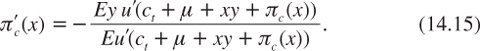
Of course, π_c(0) = 0. Differentiating equation (14.13) with respect to x yields

It implies that

The right-hand side of this equality is non-negative, since y and u′ are negatively correlated when x is positive. By the covariance rule, it implies that Eyu′ ≤ EyEu′ = 0. However, when x tends to zero, we have that This is the Arrow–Lind theorem. Marginal risks that are uncorrelated to the economy have no social cost. But what can we say about non-marginal independent risks? Differentiating equation (14.14) again implies that

Observe that the left-hand side of this equality is uniformly negative under risk aversion. It implies that the compensating risk premium is an increasing and convex function of the size of risk. This result does not hold for the classical risk premium, as shown by a counter-example presented in Eeckhoudt and Gollier (2001).

One can evaluate the error when estimating the risk premium by using the Arrow–Lind theorem. Using equation (14.16) around x = 0 and assuming μ = 0 for the sake of a simple notation, we obtain that

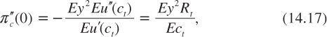
where R_t = –Ec_tEu″(c_t)/Eu’(c_t) is the risk-adjusted relative degree of risk aversion at date t. The second-order Taylor approximation of the compensated risk premium around x = 0 implies that

which is the Arrow–Pratt approximation. This means that the risk premium expressed as a percentage of initial expected consumption is approximately equal to half times the product of the variance of the relative change in consumption by the risk-adjusted relative risk aversion. For example, if the standard deviation of the cash flow of the project equals 5% of aggregate consumption, and relative risk aversion equals 2, the risk premium is approximately equal to one-fourth of a percent of aggregate consumption. As explained earlier in this book, this approximation is exact when y is log normally distributed, c_t is constant, and the utility function belongs to the CRRA family.

SUMMARY OF MAIN RESULTS

1.  Cost-benefit analysis is based on the marginalist approach. It can be used only if the investment project under evaluation is marginal, i.e., if its implementation does not affect equilibrium prices in the economy. The evaluation of non-marginal projects must be done by measuring their impact on the social welfare function.

2.  A non-marginal investment project with positive future cash flows will have an impact on welfare that is smaller than when estimated by using the standard discounting method. This is because implementing the project will increase economic growth. This will in turn increase the discount rate through the wealth effect.

3.  The risk premium associated with a risky non-marginal project will be larger than by using the CCAPM approach. This is because the (compensated) risk premium is convex in the size of risk.

REFERENCES

Arrow, K. J., and R. C. Lind (1970), Uncertainty and the evaluation of public investment decision, American Economic Review, 60, 364–378.

Dietz, S., and C. Hepburn (2010), On non-marginal cost-benefit analysis, Grantham Research Institute on Climate Change and the Environment, WP18.

Dietz S., C. Hope, and N. Patmore (2007), Some economics of “dangerous” climate change: reflections on the Stern Review, Global Environmental Change, 17, 311–325.

Eeckhoudt, L., and C. Gollier (2001), Which shape for the cost curve of risk? Journal of Risk and Insurance, 68, 387–402.

Gollier, C. (2011), Discounting and risk adjusting non-marginal investment projects, European Review of Agricultural Economics, 38 (3), 297–324.

Nordhaus, W. D. (2008), A Question of Balance: Weighing the Options on Global Warming Policies, New Haven, CT: Yale University Press.

Nordhaus, W. D., and J. Boyer (2000), Warming the World: Economic Models of Global Warming, Cambridge, MA: MIT Press.

Stern, N. (2007), Stern Review: The Economics of Climate Change, Cambridge: Cambridge University Press.

Tol, R.S.J. (2005), The marginal damage costs of carbon dioxide emissions: an assessment of the uncertainties, Energy Policy, 33 (16), 2064–2074.