Real-Time Operating Systems for DSP
In the early days of DSP, much of the software written was low level assembly language that ran in a loop performing a relatively small set of functions. There are several potential problems with this approach:
• The algorithms could be running at different rates. This makes scheduling the system difficult using a “polling” or “super loop” approach.
• Some algorithms could overshadow other algorithms, effectively starving them. With no resource management, some algorithms could never run.
• There are no guarantees of meeting real-time deadlines. Polling in the fashion described is nondeterministic. The time it takes to go through the loop may be different each time because the demands may change dynamically.
• No or difficult interrupt preemption.
• Unmanaged interrupt context switch.
• “Super loop” approach is difficult to understand and maintain.
As application complexity has grown, the DSP is now required to perform very complex concurrent processing tasks at various rates. A simple polling loop to respond to these rates has become obsolete. Modern DSP applications must respond quickly to many external events, be able to prioritize processing, and perform many tasks at once. These complex applications are also changing rapidly over time, responding to ever changing market conditions. Time to market has become more important than ever. DSP developers, like many other software developers, must now be able to develop applications that are maintainable, portable, reusable, and scalable.
Modern DSP systems are managed by real-time operating systems that manage multiple tasks, service events from the environment based on an interrupt structure, and effectively manage the system resources.
What Makes an OS an RTOS?
An operating system is a computer program that is initially loaded into a processor by a boot program. It then manages all the other programs in the processor. The other programs are called applications or tasks. (I’ll describe tasks in more detail later.)
The operating system is part of the system software layer (Figure 8.1). The function of the system software is to manage the resources for the application. Examples of system resources that must be managed are peripherals like a DMA, HPI, or on-chip memory. The DSP is a processing resource to be managed and scheduled like other resources.
The system software provides the infrastructure and hardware abstraction for the application software. As application complexity grows, a real-time kernel can simplify the task of managing the DSP MIPS efficiently using a multitasking design model. The developer also has access to a standard set of interfaces for performing I/O as well as handling hardware interrupts.
Migration to next generation processors is also easier because of the hardware abstraction provided by a real-time kernel and associated peripheral support software.
The applications make use of the operating system by making requests for services through a defined application program interface (API).
A general-purpose operating system performs these services for applications:
• In a multitasking operating system where multiple programs can be running at the same time, the operating system determines which applications should run in what order and how much time should be allowed for each application before giving another application a turn.
• It manages the sharing of internal memory among multiple applications.
• It handles input and output to and from attached hardware devices, such as hard disks, printers, and dial-up ports.
• It sends messages to each application or interactive user about the status of operation and any errors that may have occurred.
• It can offload the management of what are called batch jobs (for example, printing) so that the initiating application is freed from this work.
• On computers that can provide parallel processing, an operating system can manage how to divide the program so that it runs on more than one processor at a time.
In some respects, almost any general-purpose operating system (Microsoft’s Windows NT for example) can be evaluated for its real-time operating system qualities. But, here we will define a real-time operating system (RTOS) to be a specialized type of operating system that guarantees a certain capability within a specified time constraint.
An operating system must have certain properties to qualify it as a real-time operating system. Most importantly, a RTOS must be multithreaded and pre-emptible. The RTOS must also support task priorities. Because of the predictability and determinism requirements of real-time systems, the RTOS must support predictable task synchronization mechanisms. A system of priority inheritance must exist to limit any priority inversion conditions. Finally, the RTOS behavior should be known to allow the application developer to accurately predict performance of the system1. The purpose of a RTOS is to manage and arbitrate access to global resources such as the CPU, memory, and peripherals. The RTOS scheduler manages MIPS and realtime aspects of the processor. The memory manager allocates, frees, and protects code and memory. The RTOS drivers manage I/O devices, timers, DMAs, and so on. Aside from that, real-time operating systems do very little explicit resource management to provide acceptable predictability of task completion times.
Selecting an RTOS
A good RTOS is more than a fast kernel! Execution efficiency is only part of the problem. You also need to consider cost of ownership factors. Having the best interrupt latency or context switch time won’t seem so important if you find the lack of tool or driver support puts your project months behind schedule.
Here are some points to consider:
Is it specialized for DSP? Some real-time operating systems are created for a special applications such as DSP or even a cell phone. Others are more general-purpose operating systems. Some of the existing general-purpose operating systems claim to be real-time operating systems.
How good is the documentation and support?
How good is the tool support? The RTOS should also be delivered with good tools to develop and tune the application.
How good is the device support? Are there drivers for the devices you plan to use? For those you are most likely to add in the future?
Can you make it fit? More than general-purpose operating systems, RTOS should be modular and extensible. In embedded systems the kernel must be small because it is often in ROM and RAM space may be limited. That is why many RTOSs consist of a micro kernel that provides only essential services:
Is it certifiable? Some systems are safety critical and require certification, including the operating system
DSP Specializations
Choosing a DSP-oriented RTOS can have many benefits. A typical embedded DSP application will consist of two general components, the application software and the system software.
DSP RTOSs have very low interrupt latency. Because many DSP systems interface with the external environment, they are event or interrupt driven. Low overhead in handling interrupts is very important for DSP systems. For many of the same reasons, DSP RTOSs also ensure that the amount of time interrupts are disabled is as short as possible. When interrupts are disabled (context switching, etc) the DSP cannot respond to the environment.
A DSP RTOS also has very high performance device independent I/O. This involves basic I/O capability for interacting with devices and other threads. This I/O should also be asynchronous, have low overhead, and be deterministic in the sense that the completion time for an I/O transfer should not be dependent on the data size.
A DSP RTOS must also have specialized memory management. A DSP RTOS should provide the capability to define and configure system memory efficiently.
Capability to align memory allocations and multiple heaps with very low space overhead is important. The RTOS will also have the capability to interface to the different types of memory that may be found in a DSP system, including SRAM, SDRAM, fast on chip memory, etc.
A DSP RTOS is more likely to include an appropriate Chip Support Library (CSL) for your device. I’ll discuss CSLs in more detail later in this chapter.
Concepts of RTOS
Real-time operating systems require a set of functionality to effectively perform their function, which is to be able to execute all of their tasks without violating specified timing constraints. This section describes the major functions that real-time operating systems perform.
Task-Based
A task is a basic unit of programming that an operating system controls. Each different operating system may define a task slightly differently. A task implements a computation job and is the basic unit of work handled by the scheduler. The kernel creates the task, allocates memory space to the task and brings the code to be executed by the task into memory. A structure called a task control block (TCB) is created and used to manage the schedule of the task. A task is placeholder information associated with a single use of a program that can handle multiple concurrent users. From the program’s point-of-view, a task is the information needed to serve one individual user or a particular service request.
Periodic – Executes regularly according to a precomputed schedule.
Sporadic – Triggered by external events or conditions, with a predetermined maximum execution frequency.
Spontaneous – Optional real-time tasks that are executed in response to external events (or opportunities), if resources are available.
Multitasking
Today’s microprocessors can only execute one program instruction at a time. But because they operate so fast, they can be made to appear to run many programs and serve many users simultaneously. This illusion is created by rapidly multiplexing the processor over the set of active tasks. The processor operates at speeds that make it seem as though all of the user’s tasks are being performed at the same time.
While all multitasking depends on some time of processor multiplexing, there are many strategies for “scheduling” the processor. In systems with priority-based scheduling, each task is assigned a priority depending on its relative importance, the amount of resources it is consuming, and other factors. The operating system preempts tasks having a lower priority value so that a higher priority task is given a chance to run. I’ll have much more to say about scheduling later in this chapter.
Rapid Response to Interrupts
An interrupt is a signal from a device attached to a computer or from a program within the computer that causes the RTOS to stop and figure out what to do next. Almost all DSPs and general-purpose processors are interrupt-driven. The processor will begin executing a list of computer instructions in one program and keep executing the instructions until either the task is complete or cannot go any further (waiting on a system resource for example) or an interrupt signal is sensed. After the interrupt signal is sensed, the processor either resumes running the program it was running or begins running another program.
An RTOS has code that is called an interrupt handler. The interrupt handler prioritizes the interrupts and saves them in a queue if more than one is waiting to be handled. The scheduler program in the RTOS then determines which program to give control to next.
An interrupt request (IRQ) will have a value associated with it that identifies it as a particular device. The IRQ value is an assigned location where the processor can expect a particular device to interrupt it when the device sends the processor signals about its operation. The signal momentarily interrupts the processor so that it can decide what processing to do next. Since multiple signals to the processor on the same interrupt line might not be understood by the processor, a unique value must be specified for each device and its path to the processor.
In many ways, interrupts provide the “energy” for embedded real-time systems. The energy is consumed by the tasks executing in the system. Typically, in DSP systems, interrupts are generated on buffer boundaries by the DMA or other equivalent hardware. In this way, every interrupt occurrence will ready a DSP RTOS task that iterated on full/empty buffers. Interrupts come from many sources (Figure 8.2) and the DSP RTOS must effectively manage multiple interruptions from both inside and outside the DSP system.
RTOS Scheduling
The RTOS scheduling policy is one of the most important features of the RTOS to consider when assessing its usefulness in a real-time application. The scheduler decides which tasks are eligible to run at a given instant, and which task should actually be granted the processor. The scheduler runs on the same CPU as the user tasks and this is already the penalty in itself for using its services. There are a multitude of scheduling algorithms and scheduler characteristics. Not all of these are important for a real-time system.
A RTOS for DSP requires a specific set of attributes to be effective. The task scheduling should be priority based. A task scheduler for DSP RTOS has multiple levels of interrupt priorities where the higher priority tasks run first. The task scheduler for DSP RTOS is also preemptive. If a higher priority task becomes ready to run, it will immediately pre-empt a lower priority running task. This is required for real-time applications. Finally, the DSP RTOS is event driven. The RTOS has the capability to respond to external events such as interrupts from the environment. DSP RTOS can also respond to internal events if required.
Task states
Further refinement comes when we allow tasks to have states other than ready for execution. The major states of a typical RTOS include:
• Sleeping – The thread is put into a sleeping state immediately after it is created and initialized. The thread is released and leaves this state upon the occurrence of an event of the specified type(s). Upon the completion of a thread that is to execute again it is reinitialized and put in the sleeping state.
• Ready – The thread enters the ready state after it is released or when it is pre-empted. A thread in this state is in the ready queue and eligible for execution. (The RTOS may also keep a number of ready queues. In fixed-priority scheduling, there will be a queue for each priority. The RTOS scheduler rather than simply admitting the tasks to the CPU, makes a decision based on the task state and priority.)
• Executing – A thread is in the executing state when it executes
• Suspended (Blocked) – A thread that has been released and is yet to complete enters the suspended or blocked state when its execution cannot proceed for some reason. The kernel puts a suspended thread in the suspended queue. There are various reasons for a multitasking DSP to suspend. A task may be blocked due to resource access control. A task may be waiting to synchronize execution with some other task(s). The task may be held waiting for some reason (I/O completion and jitter control). There may be no budget or aperiodic 2 job to execute (this is a form of bandwidth control). The RTOS maintains different queues for tasks suspended or blocked for different reasons (for example, a queue for tasks waiting for each resource).
• Terminated – A thread that will not execute again enters the terminated state when it completes. A terminated thread may be destroyed.
Different RTOS’s will have slightly different states. Figure 8.3 shows the state model for a DSP RTOS, DSP/BIOS, called DSP/BIOS from Texas Instruments.
Most RTOSs provide the user the choice of round-robin or FIFO scheduling of threads of equal priority. A time slice (execution budget) is used for round-robin scheduling. At each clock interrupt the scheduler reduces the budget of the thread by the tick size. Tasks will be pre-empted if necessary (A FIFO scheduling algorithm uses an infinite time slice.) At each clock interrupt, the RTOS scheduler updates the ready queue and either returns control to the current task or preempts the current task if it is no longer the highest priority ready task. Because of the previous actions, some threads may become ready (released upon timer expiration) and the thread executing may need to be pre-empted. The scheduler updates the ready queue accordingly and then gives control to the thread at the head of the highest priority queue.
Cyclic executives (also called interrupt control loops) were until recently a popular method for designing simple DSP based real-time systems. The “cyclic” name comes from the way the control loop “cycles” through a predetermined path in the code in a very predictable manner. It is a very simple architecture because there is minimal “executive” code in the system which leads to minimal system overhead. These types of systems require only a single regular (periodic) interrupt to manage the control loop.
Steps in cyclic executive system model
An example of a cyclic executive is shown in Figure 8.4. Cyclic executive systems will generally perform one-time start-up processing (including enabling the system interrupt). The system then enters an infinite loop. Each cycle through the loop (after the first cycle) is initiated by a periodic interrupt. During each cycle, the system will first accept any required input. Application processing is then performed on the data read into the system. The resulting outputs are then generated. At the end of the cycle, the software enters an idle loop waiting for the interrupt to initiate the next cycle. During this idle time, the system could perform some low level built-in-test processing.
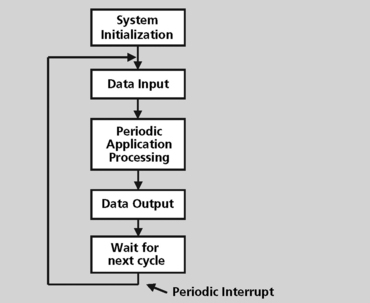
Disadvantages to cyclic executive system model
This basic cyclic executive system model is effective for simple systems where all processing is done at the rate established by the periodic interrupt. It may be unnecessary, or even undesirable, to run all “tasks” at this same rate. This is one of the drawbacks of this model – inefficiency.
This has an effect on the timing of the data output. If each task in the system has a different execution time, the timing of the data output, in relation to the regular period of the process, varies. This effect is called jitter and will occur on alternate cycles through the system. Depending on the amount of this jitter and the sensitivity of the system this effect may be totally unsatisfactory for a real-time system. One solution is to pad the shorter running task(s) with worthless computations to add time until it the shorter running task(s) take the same amount of time to complete as the other task(s). This is another inelegant approach to solving this synchronization problem. If a change is made to one of the tasks, the timing of the system may have to be adjusted to reestablish the output timing stability.
Advantages to cyclic executive system model
The Cyclic executive approach has some advantages. The model is conceptually simple and potentially very efficient, requiring relatively little memory and processing overhead.
Disadvantages to cyclic executive system model
Despite the advantages to this approach, cyclic executives have some serious disadvantages. It is very difficult to develop systems of any complexity with this model because the cyclic executive model does not support arbitrary task processing rates. All of the tasks in the system must run at a rate that is a harmonic of the periodic interrupt. Cyclic executives also require even simple control flow relationships to be hard coded into the program flowing from lower task rates to higher task rates. Because cyclic executives are nonpreemptive, the system developer must divide the lower rate processing into sometimes unnatural “tasks” that can be run each cycle. Cyclic executives do not support aperiodic processing required by many DSP-based real-time systems. It is very difficult and error-prone to make changes to the system once it is working. Even relatively small changes to the system may result in extensive repartitioning of activities, especially if the processor loading is high, to achieve system stability again. Any changes in processing time in the system can affect the relative timing of input or output operations. This will require revalidating the behavior of any control law parameters in the system. Any changes to the application requires that a timing analysis must be performed to prevent any undesirable side effects on the overall system operation.
The RTOS Kernel
A kernel can be defined as the essential center of an operating system. The kernel is the core of an operating system that provides a set of basic services for the other parts of the operating system. A kernel consists of a basic set of functions:
• An interrupt handler to handle the requests that compete for the kernel’s services.
• A scheduler to determine which tasks share the kernel’s processing time and in which order they shall use this time.
• A manager of resources that manage system resources usage such as memory or storage and how they shall be shared among the various tasks in the system.
There may be other components of operating systems such as file managers, but these are considered outside the essential requirements of the kernel needed for core processing capability.
A RTOS consists of a kernel that provides the basic operating system functions. There are three reasons for the kernel to take control from the executing thread and execute itself:
The general priority of an RTOS scheduling service is as follows (Figure 8.5):
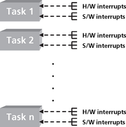
Figure 8.5 The relative priority of activity in a DSP RTOS; hardware interrupts, software interrupts, and tasks
Highest priority: Hardware interrupts – Hardware interrupts have the highest priority. One hardware interrupt can interrupt another.
Next Highest Priority: Software interrupts – The RTOS may also support a number of software interrupts. Software interrupts have a lower priority than hardware interrupts and are prioritized within themselves. A higher software interrupt can pre-empt a lower priority software interrupt. All hardware interrupts can pre-empt software interrupts. A software interrupt is similar to a hardware interrupt and is very useful for real-time multitasking applications. These interrupts are driven by an internal RTOS clock module. Software interrupts run to completion and do not block and cannot be suspended.
Next Highest Priority: Tasks – Tasks have lower priority than software interrupts. Tasks can also be pre-empted by higher priority tasks. Tasks will run to completion or yield if blocked waiting for a resource or voluntarily to support certain scheduling algorithms such as round robin.
System Calls
The application can access the kernel code and data via application programming interface (API) functions. An API is the specific method prescribed by a computer operating system or by an application program by which a programmer writing an application program can make requests of the operating system or another application. A system call is a call to one of the API functions. When this happens, the kernel saves context of calling task, switches from user mode to kernel mode (to ensure memory protection), executes the function on behalf of the calling task, and returns to user mode. Table 8.1 describes some common APIs for the DSP/BIOS RTOS.
Table 8.1
Example APIs for DSP/BIOS RTOS
| API Name | Function |
| ATM_cleari, ATM_clearu | Atomically clear memory location and return the previous value |
| ATM_seti, ATM_setu | Atomically set memory and return previous value |
| CLK_countspms | Number of hardware timer counts per millisecond |
| CLK_gethtime, CLK_getltime | Get high and low resolution time |
| HWI_denable, HWI_disable | Globally enable and disable hardware interrupts |
| LCK_create, LCK_delete | Create and delete a resource lock |
| LCK_pend, LCK_post | Aquire and relinquish ownership of a resource lock |
| MBX_create, MBX_delete, MBX_pend, MBX_post | Create, delete, wait for a message, and post a message to a mailbox |
| MEM_alloc, MEM_free | Allocate from a memory segment, free a block of memory |
| PIP_get, PIP_put | Get and put a frame into a pipe |
| PRD_getticks, PRD_tick | Set the current tick counter, Advance the tick counter and dispatch periodic functions |
| QUE_Create, QUE_delete, QUE_dequeue, QUE_empty | Create and delete an empty queue, remove from front of queue and test for an empty queue |
| SEM_pend, SEM_post | Wait for and signal a semaphore |
| SIO_issue, SIO_put | Send and put a buffer to a stream |
| SWI_enable, SWI_getattrs | Enable software interrupts, Get attributes of a software interrupt |
| SYS_abort, SYS_error | Abort program execution, flag error condition |
| TSK_create, TSK_delete | Create a task for execution, delate a task |
| TSK_disable, TSK_enable | Disable and enable the RTOS scheduler |
| TSK_getenr, TSK_setpri | Get the task environment, set a task priority |
Dynamic Memory Allocation
Dynamic memory allocation allows the allocation of memory at variable addresses. The actual address of the memory is usually not a concern to the application. One of the disadvantages of dynamic memory allocation is the potential for memory fragmentation. This occurs when there is enough memory in total but an allocation of a memory block fails due to lack of a single large enough block of memory. RTOS must manage the heap effectively to allow maximum use of the heap.
Chip Support Software for DSP RTOS
A part of the DSP RTOS support infrastructure is software to support the access of the various chip peripherals. This Chip Support Library (CSL) is a runtime library used to configure and control all of the DSP on-chip peripherals such as the cache, DMA, external memory interface (EMIF), multichannel buffered serial port (MCBSP), the timers, high speed parallel interfaces (HPI), etc. The CSL provides the peripheral initialization as well as the runtime control. This software fits well into a DSP RTOS package to provide the necessary abstraction from the hardware that the DSP programmer requires to be productive and effective. DSP vendors can provide this software written (mostly) in C and already optimized for code size and speed. Figure 8.6 shows how the CSL fits into the DSP RTOS infrastructure.
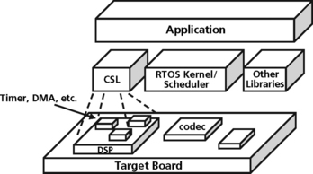
Figure 8.6 Chip Support Library to support a DSP RTOS infrastructure (courtesy of Texas Instruments)
Benefits for the CSL
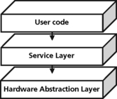
Because different DSP chips and families of chips support different peripherals (a TMS320C2x DSP device may support specific peripherals to support motor control such as a CAN device, while a DSP such as the TMS320C5x device, which is optimized for low power and portable applications, may support a different set of peripherals including a Multichannel buffered serial port for optimized I/O), a different chip support library is required for each device. The hardware abstraction provided by these libraries adds very little overhead to the system and provides several benefits to the DSP developer:
• Shortened development time – The DSP developer will not be burdened with understanding a large number of memory mapped registers for the DSP device. A hardware abstraction layer in the CSL has already defined this (Figure 8.7).
• Standardization – A properly developed CSL will have a uniform methodology for developing the API definitions to be used by the DSP developer. The level of abstraction and the coverage from a macro level will be consistent.
• Tool support – DSP tools support is often available to make the job of generating customized configuration structures and initializing registers easier.
• Resource management – Basic resource management for peripherals that have multiple channels, ports, devices, and so on is much easier.
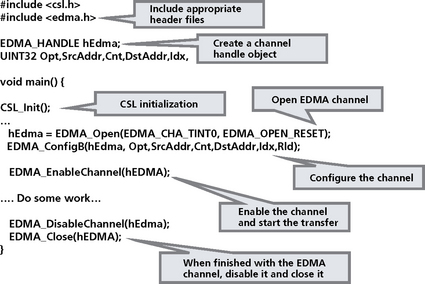
Example
Figure 8.8 is an example of a simple CSL function. This example opens an EDMA channel, configures it, and closes it when finished.
DSP RTOS Application Example
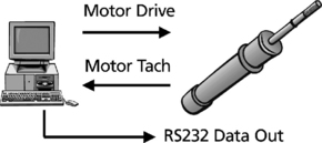
As an example of the techniques and concepts that have been discussed in this chapter, a simple motor control example will be discussed. In this example, a single DSP will be used to control a motor (Figure 8.9). The DSP will also be responsible for interfacing to an operator using a keypad, updating a simple display device, and sending data out one of the DSP ports. The operator uses the keypad to control the system. The motor speed must be sampled at a 1 KHz rate. A timer will be used to interrupt processing at this rate to allow the DSP to execute some simple motor control algorithms. At each interrupt, the DSP will read the motor speed, run some simple calculations, and adjust the speed of the motor accordingly. Diagnostic data is transmitted out the RS232 port when selected by the operator using the keypad. The summary of these motor control requirements are shown in Table 2.
Table 8.2
Summary of motor control requirements
Requirements
Control motor speed (1 KHz sampling rate - dV/dT)
Accept keyboard commands to control the motor, change the display, or send data out the RS232 port
Drive a simple display and refresh 2 times per second
Send data out the RS232 port when there is nothing else to do
Defining the Threads
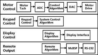
The first step in developing a multitasking system is to architect the application into isolated independent execution threads. There are tools available to help the system designer during this phase. This architecture definition will produce data flow diagrams, system block diagrams, or finite state machines. An example of a set of independent execution threads is shown in Figure 8.10. There are four independent threads in this design: the main motor control algorithm which is a periodic task, running at a 1 KHz rate, a keypad control thread which is an aperiodic task controlled by the operator, a display update thread which is a periodic task executing at a 2 Hz rate, and a data output thread which runs as a background task and outputting data when there is no other processing required.
Determining Relative Priority of Threads
Once the major threads of the application have been defined, the relative priority of the threads must be determined. Since this motor control example is a real-time system (there are hard real-time deadlines for critical operations to complete), there must be a priority assigned to the thread execution. In this example, there is one hard real-time thread, the motor control algorithm that must execute at a 1 KHz rate. There are some soft real-time tasks in the system as well. The display update at a two hertz rate is a soft-real time task (this is a soft real-time task because although the display update is a requirement, the system will not fail if the display is not updated precisely twice per second.). The keypad control is also a soft real-time task but since it is the primary control input, it should have a higher priority than the display update. The remote output thread is a background task that will run when no other task is running.
Using Hardware Interrupts
The motor control system will be designed to use a hardware interrupt to control the motor control thread. Interrupts have fast context switching times (faster than that of thread context switch) and can be generated from the timer on the DSP. The priority of the tasks in the motor control example are shown in Table 3. This is an example of a rate monotonic priority assignment; the shorter the period of the thread, the higher the priority.
Table 8.3
Assignment of priorities to motor control threads and the activation mechanisms

(courtesy of Texas Instruments)
Along with the priority, the activation mechanism is described. The highest priority motor control thread will use a hardware interrupt to trigger execution. Hardware interrupts are the highest priority scheduling mechanism in most real time operating systems (Figure 8.11). The keypad control function is an interface to the environment (operator console) and will use a hardware interrupt to signal the keypad control actions. This priority will be at a lower priority than the motor control interrupt. The display control thread will use a software interrupt to schedule a display update at a 2 hertz rate. Software interrupts operate similar to hardware interrupts but at a lower priority than hardware interrupts (but at a higher priority than threads). The lowest priority task, the remote output task, will be executed as an idle loop. This idle loop will runs continuously in the background while there are no other higher priority threads to run.
Thread Period
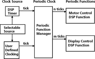
The periodicity of each thread is also described in Table 8.3. The highest priority thread, the motor control thread, is a periodic thread. Like many DSP applications this thread processes data periodically, in this case at a 1 KHz rate. This motor control example is actually a multirate system. This means there are multiple periodic operations in the system (motor control and display control, for example). These threads operate at different rates. DSP RTOSs allow for multiple periodic threads to run. Table 3 shows how the two periodic threads in this system are architected within the framework of the RTOS. For each of these threads, the DSP system designer must determine the period the specific operation must run and the time required to complete the operation. The DSP developer will then program the DSP timer functions in such a way to produce an interrupt or other scheduling approach to enable the thread to run at the desired rate. Most DSP RTOSs have a standard clock manager and API function to perform this setup operation.
Summary
The complexity of real-time systems continues to increase. As DSP developers migrate from a model of “programming in the small,” where the DSP application performs a single task, to one of “programming in the large,” where the DSP application performs a number of complicated tasks, scheduling the system resources optimally is becoming more and more difficult. An RTOS provides the needed abstraction from this complexity while providing the performance required of real-time systems. An RTOS can be configured by the DSP developer to schedule the various tasks in the system based on a set of rules, handle external events quickly and efficiently, and allocate and manage system resources.
Commercial DSP RTOSs provide a good value to the DSP developer. They come already debugged (having been used by many commercial users in the past) and with good documentation and tooling support. DSP RTOSs have also been optimized to provide the smallest footprint possible and with the best performance possible for key functions such as context switching and interrupt latency processing.
The most common DSP RTOS implement prioritized-preemptive scheduling policies. Systems based on this scheduling approach are popular in real-time systems because they are the most readily analyzed of the more sophisticated scheduling mechanisms. We will now turn our attention to the analysis of these scheduling policies.
Multiprocessing pitfalls
Multiprocessing, although required for complex real-time systems, suffers from potential dangers that must be carefully considered to prevent unexpected system performance and correctness problems. Multiprocessing problems can be very subtle and difficult to diagnose and fix. Some problems cannot be reliably removed through “debugging,” so careful design and extreme discipline are critical. A major role of the RTOS is to encapsulate as much of these problems as practical and to establish the “metaphor” used to structure the discipline.
This chapter will outline the major issues with implementing multiprocessing systems. We will first discuss the danger of deadlock. We will also discuss the ways in which multiprocessing systems share common resources. Designers of DSP-based systems and embedded systems in general must constantly manage the allocation of scarce resources; these may include on-chip memory, the DMA controller, a peripheral, an input or output buffer, etc. This chapter will introduce ways to synchronization on shared resources as well as other forms of task synchronization.
Deadlock
One common danger is that of “deadlock,” also known as deadly embrace. A deadlock is a situation in which two computer programs sharing the same resource are effectively preventing each other from accessing the resource, resulting in both programs ceasing to function. The earliest computer operating systems ran only one program at a time. In these situations, all of the resources of the system were always available to the single running program, and thus deadlock wasn’t an issue. As operating systems evolved, they began to support timesharing and to interleave the execution of multiple programs. In early timesharing systems, programs were required to specify in advance what resources they needed so that they could avoid conflicts with other programs running at the same time. Still, deadlocks weren’t a problem. But then, as timesharing systems evolved, some began to offer dynamic allocation of resources. These systems allowed a program or task to request further allocation of resources after it had begun running. Suddenly deadlock was a problem—in some cases a problem that would freeze the entire system several times a day.
The following scenario illustrates how deadlock develops and how it is related to dynamic (or partial) allocation of resources:
• Program 1 requests resource A and receives it.
• Program 2 requests resource B and receives it.
• Program 1 requests resource B and is queued up, pending the release of B.
• Program 2 requests resource A and is queued up, pending the release of A.
• Now neither program can proceed until the other program releases a resource. The OS cannot know what action to take.
At this point the only alternative is to abort (stop) one of the programs.
Deadlock Prerequisites
As our short history of operating systems illustrates, several conditions must be met before a deadlock can occur:
• Mutual exclusion – Only one task can use a resource at once.
• Multiple pend and wait – There must exist tasks which are holding resources while waiting for others.
• Circular pend – Circular chain of tasks hold resources that are needed by others in the chain (cyclic processing).
• Preemption – A resource can only be released voluntarily by a task.
Unfortunately, these prerequites are quite naturally met by almost any dynamic, multitasking system, including the average real-time embedded system.
Handling Deadlock
There are two basic strategies for handling deadlock: make the programmer responsible or make the operating system responsible. Large, general-purpose operating systems usually make it their responsibility to avoid deadlock. Small footprint RTOSs, on the other hand, usually expect the programmer to follow a discipline that avoids deadlock.
Deadlock prevention
Programmers can prevent deadlock by disciplined observance of some policy that guarantees that at least one of the prerequisites of deadlock (mutual exclusion, hold and wait, no preemption of the resource, and circular wait) can never occur in the system. The mutual exclusion condition can be removed, for example, by making resources sharable. This is difficult, if not impossible, to do in many cases. Another approach is to remove the circular pend condition. This can be solved by setting a particular order in which resources are requested (for example, all processes must request resource A before B). A third approach is to remove the multiple pend and wait conditions by requiring each task to always acquire all resources that will be used together as one “atomic” acquisition. This increases the risk of starvation and must be used carefully. Finally, you can allow preemption, in other words, if a task can’t acquire a particular resource within a certain time, it must surrender all resources it holds and try again.
Deadlock detection and recovery
Some operating systems are able to manage deadlock for the programmer, either by detecting deadlocks and recovering or by refusing to grant (avoiding) requests that might lead to deadlock. This approach is difficult because the deadlock is generally hard to detect. Resource allocation graphs can be used but this can also be a very difficult task to perform in a large real-time system. Recovery is, in most cases, not easy. One extreme approach is to reset the system Another approach is to perform a rollback to a pre-deadlock state. In general, deadlock detection is more appropriate for general-purpose operating systems than RTOSs.
Deadlock avoidance
Here the RTOS dynamically detects whether honoring a resource request could cause it to enter an unsafe state. To implement a deadlock avoidance approach, the RTOS must implement an algorithm which allows all four deadlock preconditions to occur but which will also ensure that the system never enters a deadlock state. On resource allocation, the RTOS needs to examine dynamically the resource allocation state and take action based on the possibility of deadlock occurring. The resource allocation state is the number of resources available, the number of resources allocated, and maximum demand on the resources of each process.
Shared Resource Integrity
A second hazard of concurrent programming is resource corruption. When two (or more) interleaved threads of execution both try to update the same variable (or otherwise modify some shared resource), the two threads can interfere with each other, corrupting the state of the variable or shared resource.
As an example, consider a DSP system with the following characteristics:
• Shared memory (between tasks);
• Load-store architecture (like many of the DSP architectures today);
• Two tasks running in the system, T1 and T2 (T2 has higher priority);
• Both tasks needing to increment a shared variable X by one.
There are two possible interleavings for these tasks on the system, as shown below:
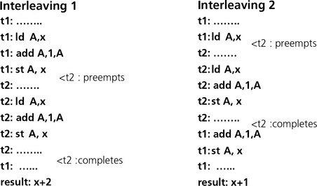
Solution—Mutual Exclusion
Interleaving 1 does not work correctly because the preemption occurred in the middle of a read/modify/write cycle. The variable X was shared between the tasks. For correct operation, any read/modify/write operation on a shared resource must be executed atomically; that is, in such a way that it cannot be interrupted or pre-empted until complete. Sections of code that must execute atomically are critical sections. A critical section is a sequence of statements that must appear to be executed indivisibly.
Another way of viewing this problem is to say that while the shared variable can be shared, it can only be manipulated or modified by one thread at a time; that is, any time one thread is modifying the variable, all other threads are excluded from access. This access discipline (or type of synchronization) is called mutual exclusion.
Synchronizing Tasks for Mutual Exclusion
There are a number of potential solutions to the synchronization requirement. Some approaches are dependent on the DSP hardware. These approaches can be very efficient but they are not always useable.
One approach is to disable interrupts. If you simply disable the DSP processor’s interrupts, then it becomes impossible to have a context switch occur since all interrupts (except for perhaps a nonmaskable interrupts, which is usually reserved for when something serious has to occur or has occurred—for example resetting the DSP) are disabled. Note that this only works if you have a single processor—multiprocessor DSP systems get more complicated and will not be discussed here.
Another approach that is hardware-related is to use an atomic instruction to record the old state of a bit, and then change its state. Some DSPs have specialized instructions referred to as test and set bit. The DSP hardware implements an instruction that does atomically what are normally a pair of operations. This instruction will examine a specified bit in memory, set a condition code depending on what that memory location contains, and then set the bit to a value of 1. This instruction, in affect, will “atomic-ize” several memory transactions in such a way that an interrupt cannot occur between the two memory transactions thereby avoiding shared data problems in multiprocessing systems.
With mutual exclusion, only one of the application processes can be in the critical section at a time (meaning having the program counter pointing to the critical section code). If no processes are in the critical section, and a process wants to enter the critical section, that process can participate in a decision making process to enter the critical section.
Other software approaches involve asking a resource manager function in an RTOS for access to the critical section. RTOSes use mechanisms called semaphores to control access. A semaphore is a synchronization variable that takes on positive integer values.
We will now discuss these approaches and the advantages and trade-offs of each.
Mutual Exclusion via Interrupt Control
One approach to mutual exclusion is proactively to take steps to prevent the task that is accessing a shared resource or otherwise executing in a critical section from being interrupted. Disabling interrupts is one approach. The programmer can disable interrupts prior to entering the critical section, and then enable interrupts after leaving the critical section:
This approach is useful because no clock interrupts occur and the process has exclusive access to the CPU and cannot be interrupted by any other process. The approach is simple and efficient.
There are some significant drawbacks to the approach. Disabling interrupts effectively turns off the preemptive scheduling ability of your system. Doing this may adversely affect system performance. The more time spent in a critical section with interrupts turned off, the greater the degradation in system latency. If the programmer is allowed to disable interrupts at will, he or she may easily forget to enable interrupts after a critical section. This leads to system hangs that may or may not be obvious. This is a very error prone process and, without the right programmer discipline, could lead to significant integration and debug problems. Finally, this approach works for single processor systems but does not work for multiprocessor systems.
RTOSs provide primitives to help a programmer manage critical sections without having to resort to messing with the system interrupts.
Mutual Exclusion with a Simple Semaphore
In its simplest form, a semaphore is just a thread safe flag that is used to signal that a resource is “locked.” Most modern instruction sets include instructions that are especially designed to so that they can be used as a simple semaphore. The two most common suitable instructions are test and set instructions and swap instructions. The critical feature is that the flag variable must be both tested and modified as a single, atomic operation.
The most primitive techique for synchronizing on a critical section is called busy waiting. In this approach, a task sets and checks a shared variable (a simple semaphore) that acts as a flag to provide synchronization. This approach is also called spinning with the flag variables called spin locks. To signal a resource (use that resource), a task sets the value of a flag and proceeds with execution. To wait for a resource, a task checks the value of the flag. If the flag is set, the task may proceed with using the resource. If the flag is not set, the task will check again.
The disadvantages of busy waits are that the tasks spend processor cycles checking conditions without doing useful work. This approach can also lead to excessive memory traffic. Finally, it can become very difficult to impose queuing disciplines if there is more than one task waiting on a condition. To work properly, the busy wait must test the flag and set it if the resource is available, as a single atomic operation. Modern architectures typically include an instruction designed with this operation in mind.
Test and set instruction
The test and set instruction is atomic by hardware design. This instruction allows a task to access a memory location in the following way:
The pseudocode for this operation is as follows:
The task must test the location for 0 before executing a wait. If the value is 0 then the task may proceed. If it is not a 0, then the task must wait. After completing the operation, the task must reset the location to 0.
Swap instruction
The swap instruction is similar to test and set. In this case, a task wishing to execute a semaphore operation will swap a 1 with the lock bit. If the task gets back a 0 (zero) from the lock, it can proceed. If the task gets back a 1 then some other task is active with the semaphore and it must retest.
The following example uses a test and set instruction in a busy wait loop to control entry to a critical section.
Mutual Exclusion via Blocking Semaphores
A blocking semaphore is a nonnegative integer variable that can be used with operating system services Wait() and Signal() to implement several different kinds of synchonization. The Wait() and Signal() services behave as follows:
• Wait(S): If the value of the semaphore, S, is greater than zero then decrement its value by one; otherwise delay the task until S is greater than zero (and then decrement its value).
• Signal(S): Increment the value of the semaphore, S, by one.
The operating system guarantees that the actions of wait and signal are atomic. Two tasks, both executing wait or signal operations on the same semaphore, cannot interfere with each other. A task cannot fail during the execution of a semaphore operation (which requires support from the underlying operating system).
When a task must wait on a blocking semaphore, the following run time support actions are performed:
• The task executes a wait (semaphore pend).
• The task is removed from the CPU.
• The task is placed in a queue of suspended tasks for that semaphore.
• Eventually a signal executes on that semaphore.
• The RTOS will pick out one of the suspended tasks awaiting a signal on that semaphore and make it executable. (The semaphore is only incremented if no tasks are suspended.)
Blocking semaphores are indivisible in the sense that once a task has started a wait or signal, it must continue until it is complete. The RTOS scheduler will not pre-empt the task when a signal or wait is executing. The RTOS may also disable interrupts so no external event interrupts it3. In multiprocessor systems, an atomic memory swap or test and set instructions are required to lock the semaphore.
Mutual exclusion via blocking semaphores removes the need for busy-wait loops. An example of this type of operation is shown below:
var mutex : semaphore; (*initially zero *)
This example allows only one task at a time to have access to a resource such as on-chip memory or the DMA controller. In Figure 8.12, the initial count for the mutual exclusion semaphore is set to one. Task 1, when accessing a critical resource, will call Pend upon entry to the critical region and call the Post operation on exit from the resource.
In summary, semaphores are software solutions—they are not provided by hardware. Semaphores have several useful properties:
• Machine independence – Semaphores are implemented in software and are one of the standard synchronization mechanisms in DSP RTOSs.
• Simple – Semaphore use is relatively simple, requiring a request and a relinquish operation which are usually API calls into the RTOS.
• Correctness is easy to determine – For complex real-time systems, this is very important.
• Works with many processes – Semaphore use is not limited by the complexity of the system.
• Different critical sections with different semaphores – Different system resources can be protected using different semaphores. This significantly reduces the system responsiveness. If all important sections of code and system resources were protected by a single semaphore, the “waiting line” to use the semaphore would be unacceptable with respect to overall system response time.
• Can acquire multiple resources simultaneously – If you have two or more identical system resources that need to be protected, a “counting” semaphore can be used to manage the “pool” of resources.
Mutual Exclusion Through Sharable Resources
All of the synchronization techniques we’ve reviewed so far have a common disadvantage: they require the programmer to follow a particular coding discipline each time they use the resource. A more reliable and maintainable solution to the mutual exclusion problem is to make the resources sharable.
Many operating systems offer fairly high-level, sharable data structures, including queues, buffers, and data pipes that are guaranteed thread safe because they can only be accessed through synchronized operating system services.
Circular Queue or Ring Buffer
Often, information can be communicated between tasks without requiring explicit synchronization if the information is transmitted via a circular queue or ring buffer. This type of buffer is viewed as a ring of items. The data is loaded at the tail of the ring buffer. Data is read from the head of the buffer. This type of buffer mechanism is used to implement FIFO request queues, data queues, circulating coefficients, and data buffers. An example of the logic for this type of buffer is shown below.
Pseudocode for a Ring Buffer
The advantage of this structure is that if pointer updates are atomic and the queue is shared between only a single reader and writer, then no explicit synchronization is necessary. As with any finite (bounded) buffer, the readers and writers must be careful to observe two critical correctness conditions:
• The producer task must not attempt to deposit data into the buffer if the buffer is full.
• The consumer task cannot be allowed to extract objects from the buffer if the buffer is empty.
If multiple readers or writers are allowed, explicit mutual exclusion must be ensured so that the pointers are not corrupted.
Double Buffering
Double buffering (often referred to as ping pong buffering) is the use of two equal buffers where the buffer being written to is switched with the buffer being read from and alternately back. The switch between buffers can be performed in hardware or software.
This type of buffering scheme can be used when time-relative data needs to be transferred between cycles of different rates, or when a full set of data is needed by one task but can only be supplied slowly by another task. Double buffering is used in many telemetry systems, disk controllers, graphical interfaces, navigational equipment, robot controls and other applications. Many graphics displays, for example, use two buffers where the buffer being written to is switched with the buffer being read from and alternately back. The switch can be performed in hardware or software.
Data Pipes
As an example of support for data transfer between tasks in a real-time application, DSPBIOS provides I/O building blocks between threads (and interrupts) using a concept called pipes.
A pipe is an object that has 2 sides, a “tail,” which is the producer side and a “head,” which is the consumer side (Figure 8.13). There are also “notify functions” that are called when the system is ready for I/O. The data buffer used in this protocol can be divided into a fixed number of frames, referred to as “nframes” as well as a frame size, “framesize.”

A separate pipe should be used for each data transfer thread (Figure 8.14). A pipe should have a single reader and a single writer (point to point protocol). The notify function can perform operations on the software interrupt mailbox. During program startup, a notifywriter function is called for each pipe.
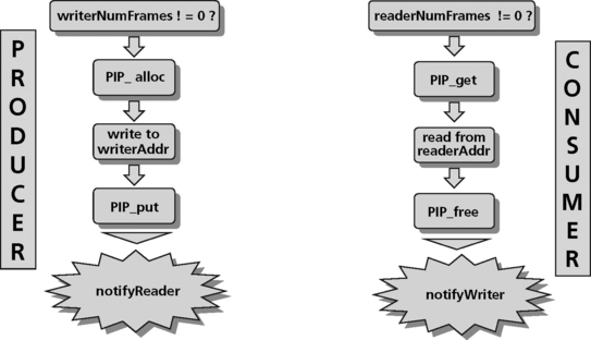
Writing to a pipe
To write to a pipe, a function first checks the writerNumFrames in the pipe object to make sure at least one empty frame is available. The function calls PIP_alloc to get an empty frame. If more empty frames are available, PIP_alloc will run the notifywriter function for each frame. The function writes the data to the address pointed to by writerAddr up to writerSize. Finally, the function should call PIP_put to put the frame in the pipe. Calling PIP_put will call the notifyReader function to synchronize with the consumer. (Figure 8.14).
Reading from a pipe
To read from a pipe, a function first checks the readerNumFrames in the pipe object to ensure at least one full frame is available. The function calls PIP_get to get a full frame from the pipe. If more full frames are available PIP_alloc will run the notifyReader function for each frame. The function reads the data pointed to by the readerAddr up to readerSize. Finally, the function calls PIP_free to recycle the frame for reuse by PIP_alloc. Calling PIP_free will call the notifyWriter function to synchronize with the producer (Figure 8.14).
Example
As an example, consider part of a telecommunications system that transforms an 8 KHz input (voice) stream into a 1 KHz output (data) stream using an 8:1 compression algorithm operating on 64 point data frames. There are several tasks that can be envisioned for this system:
1. 1There must be an input port that is posted by a periodic interrupt at an 8 KHz rate. (Period = 0.125 msec). An input device driver will service this port and pack the frames with 64 data points. This is task 1.
2. There is an output port that is updated by a posted periodic interrupt at a 1 KHz rate. (Period = 1 msec). An output device driver will service this port and unpack the 8 point output frames. This is task 2.
3. Task 3 is the compression algorithm at the heart of this example that executes once every 8 ms. (64 * 0.125 and 8 *1). It needs to be posted when both a full frame and an empty frame are available. Its execution time needs to be considerably less than 8 msec to allow for other loading on the DSP.
The tasks are connected by two pipes, one from task 1 to task 3 and one from task 3 to task 1. Pipe one will need two frames of 64 data words. Pipe two will need two frames of 8 data words.
When the input device driver has filled a frame, it notifies the pipe by doing a PIP_put call to pipe 1. Pipe 1 signals to task 3 using a SIG_andn call to clear a bit to indicate a full input frame. Task 3 will post if the bit indicating an empty frame is already zero.
When the output device driver has emptied a frame, it notifies the pipe by doing a PIP_free call to pipe 1. Pipe 1 posts to task 3 using a SIG_andn call to clear a bit to indicate an empty output frame. Task 3 will post if the bit indicating a full frame is available is already zero. The pseudocode for these tasks is shown below.
if (‘current frame is full’) {
PIP_put(inputPipe); /* enqueue current full frame */
PIP_alloc(inputPipe); /* dequeue next empty frame */
HWI_exit; /* dispatch pending signals */
if (‘current frame is empty’) {
PIP_free(outputPipe); /* enqueue current empty frame */
PIP_get(outputPipe); /* dequeue next full frame */
HWI_exit; /* dispatch pending signals */
compressionSignal(inputPipe, outputPipe){
PIP_get(inputPipe); /* dequeue full frame */
PIP_alloc(outputPipe); /* dequeue empty frame */
do compression algorithm /* read/write data frame */
PIP_free(inputPipe); /* recycle input frame */
Pseudocode for Telecommunication System Tasks
Note that the communication and synchronization is independent of the nature of the input drivers, the compression routine, or even whether the input/output interrupts are really every data point (other than frame sizes).
Other Kinds of Synchronization
While shared resources are the primary reason tasks need to synchronize their activity, there are other situations where some form of synchronization is necessary. Sometimes one task needs to wait for others to complete before it can proceed (rendezvous). Sometimes a task should proceed only if certain conditions are met (conditional). The following sections explain how to achieve these kinds of synchronization.
Task Synchronization (Rendezvous)
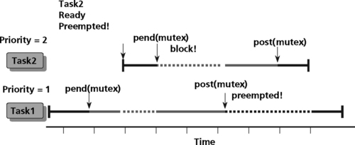
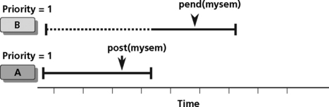
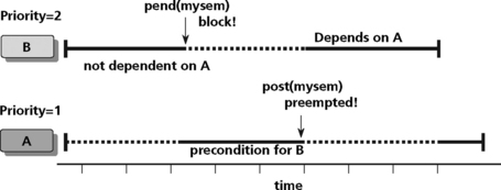
Semaphores are often used for task synchronization. Consider the case of two tasks executing in a DSP. Both tasks have the same priority. If task A becomes ready before task B, task A will post a semaphore and task B will pend on the synchronization semaphore, as shown in Figure 8.15. If task B has a higher priority than task A and task B is ready before task A, then task A may be pre-empted after releasing a semaphore using the Post operation (Figure 8.16).
Conditional Synchronization
Conditional synchronization overview
Conditional synchronization is a type of synchronization that is needed when a task wishes to perform an operation that can only logically, or safely, be performed if another task has itself taken some action or is some defined state. An example of this type of synchronization is a buffer. A buffer is used to link (decouple) two tasks, one of which writes data that the other which reads data. The use of a buffer link is known as a producer-consumer system. A buffer can be used for efficient handling of fluctuations of speed between the tasks, different data sizes between consumer and producer, preserving time relativeness, and re-ordering of data.
An example of conditional synchronization using semaphores is shown below;
Summary
Current execution (multiprocessing) provides many benefits to the development of complex real-time systems. However, one of the significant problems with multiprocessing is that concurrent processes often need to share data (maintained in data structures in shared memory) as well as resources such as on-chip memory, or an I/O port or peripheral. There must be controlled access to this shared data or resource or some processes may obtain an inconsistent view of the data or incorrectly use the hardware resource. The actions performed by the concurrent processes will ultimately depend on the order in which their execution is interleaved. This leads to nondeterminism in their execution, which is catastrophic for real-time systems and may be extremely hard to diagnose and correct.
Concurrency errors can be very subtle and intermittent. It is very important to identify and properly synchronize everything shared among threads or tasks. One of the advantages of an RTOS is to make this problem more manageable.
The DSP RTOS manages mutual-exclusion in multiprocessing systems by guaranteeing that critical sections will not be executed by more than one process simultaneously. These sections of code usually access shared variables in a common store or access shared hardware like on-chip DSP memory or the DMA controller. What actually happens inside the critical section is immaterial to the problem of mutual-exclusion. For real-time systems there is usually an assumption that the section is fairly short in order to reduce overall system responsiveness.
Semaphores are used for two main purposes in real-time DSP systems: task synchronization and resource management. A DSP RTOS implements sempahore mechanisms. The application programmer is responsible for the proper management of the resources, but the semaphore can be used as an important tool in this management.
Schedulability and Response Times
So far we’ve said that determinism was important for analysis of real-time systems. Now we’re going to show you the analysis. In real-time systems, the process of verifying whether a schedule of task execution meets the imposed timing constraints is referred to as schedulability analysis. In this chapter, we will first review the two main categories of scheduling algorithms, static and dynamic. Then we will look at techniques to actually perform the analysis of systems to determine schedulability. Finally, we will describe some methods to minimize some of the common scheduling problems when using common scheduling algorithms.
Scheduling Policies in Real-Time Systems
There are several approaches to scheduling tasks in real-time systems. These fall into two general categories, fixed or static priority scheduling policies and dynamic priority scheduling policies.
Many commercial RTOSs today support fixed-priority scheduling policies. Fixed-priority scheduling algorithms do not modify a job’s priority while the task is running. The task itself is allowed to modify its own priority for reasons that will become apparent later in the chapter. This approach requires very little support code in the scheduler to implement this functionality. The scheduler is fast and predictable with this approach. The scheduling is mostly done offline (before the system runs). This requires the DSP system designer to know the task set a-priori (ahead of time) and is not suitable for tasks that are created dynamically during run time. The priority of the task set must be determined beforehand and cannot change when the system runs unless the task itself changes its own priority.
Dynamic scheduling algorithms allow a scheduler to modify a job’s priority based on one of several scheduling algorithms or policies. This is a more complicated approach and requires more code in the scheduler to implement. This leads to more overhead in managing a task set in a DSP system because the scheduler must now spend more time dynamically sorting through the system task set and prioritizing tasks for execution based on the scheduling policy. This leads to nondeterminism, which is not favorable, especially for hard real-time systems. Dynamic scheduling algorithms are online scheduling algorithms. The scheduling policy is applied to the task set during the execution of the system. The active task set changes dynamically as the system runs. The priority of the tasks can also change dynamically.
Static Scheduling Policies
Examples of static scheduling policies are rate monotonic scheduling and deadline monotonic scheduling. Examples of dynamic scheduling policies are earliest deadline first and least slack scheduling.
Rate-monotonic scheduling
Rate monotonic scheduling is an optimal fixed-priority policy where the higher the frequency (1/period) of a task, the higher is its priority. This approach can be implemented in any operating system supporting the fixed-priority preemptive scheme, such as DSP/BIOS and VxWorks. Rate monotonic scheduling assumes that the deadline of a periodic task is the same as its period. Rate monotonic scheduling approaches are not new, being used by NASA, for example, on the Apollo space missions.
Dynamic Scheduling Policies
Dynamic scheduling algorithms can be broken into two main classes of algorithms. The first is referred to as a “dynamic planning based approach.” This approach is very useful for systems that must dynamically accept new tasks into the system; for example a wireless base station that must accept new calls into the system at a some dynamic rate. This approach combines some of the flexibility of a dynamic approach and some of the predictability of a more static approach. After a task arrives, but before its execution begins, a check is made to determine whether a schedule can be created that can handle the new task as well as the currently executing tasks. Another approach, called the dynamic best effort apprach, uses the task deadlines to set the priorities. With this approach, a task could be pre-empted at any time during its execution. So, until the deadline arrives or the task finishes execution, we do not have a guarantee that a timing constraint can be met. Examples of dynamic best effort algorithms are Earliest Deadline First and Least Slack scheduling.
Earliest deadline first scheduling
Earliest deadline first scheduling is a dynamic priority preemptive policy. With this approach, the deadline of a task instance is the absolute point in time by which the instance must complete. The task deadline is computed when the instance is created. The operating system scheduler picks the task with the earliest deadline to run. A task with an earlier deadline preempts a task with a later deadline.
Least slack scheduling
Least slack scheduling is also a dynamic priority preemptive policy. The slack of a task instance is the absolute deadline minus the remaining execution time for the instance to complete. The OS scheduler picks the task with the shortest slack to run first. A task with a smaller slack preempts a task with a larger slack. This approach maximizes the minimum lateness of tasks.
Dynamic priority preemptive scheduling
In a dynamic scheduling approach such as dynamic priority preemptive scheduling, the priority of a task can change from instance to instance or within the execution of an instance. In this approach a higher priority task preempts a lower priority task. Very few commercial RTOS support such policies because this approach leads to systems that are hard to analyze for real-time and determinism properties. This section will focus instead on static scheduling policies.
Scheduling Periodic Tasks
Many DSP systems are multirate systems. This means there are multiple tasks in the DSP system running at different periodic rates. Multirate DSP systems can be managed using nonpreemptive as well as preemptive scheduling techniques. Nonpreemptive techniques include using state machines as well as cyclic executives.
Analyzing Scheduling Behavior in Preemptive Systems
Preemptive approaches include using scheduling algorithms similar to the ones just described (rate monotonic scheduling, deadline monotonic scheduling, etc). This section will overview techniques to analyze a number of tasks statically in a DSP system in order to schedule them in the most optimal way for system execution. In the sections that follow, we’ll look at three different ways of determining whether a particular set of tasks will meet it’s deadlines: rate monotonic analysis, completion time analysis, and response time analysis.
Rate Monotonic Analysis
Some of the scheduling strategies presented earlier presented a means of scheduling but did not give any information on whether the deadlines would actually be met.
Rate Monotonic analysis addresses how to determine whether a group of tasks, whose individual CPU utilization is known, will meet their deadlines. This approach assumes a priority preemption scheduling algorithm. The approach also assumes independent tasks. (no communication or synchronization).4
In this discussion, each task discussed has the following properties:
• Each task is a periodic task which has a period T, which is the frequency with which it executes.
• An execution time C, which is the CPU time required during the period.
A task is schedulable if all its deadlines are met (i.e., the task completes its execution before its period elapses.) A group of tasks is considered to be schedulable if each task can meet its deadlines.
Rate monotonic analysis (RMA) is a mathematical solution to the scheduling problem for periodic tasks with known cost. The assumption with the RMA approach is that the total utilization must always be less than or equal to 100%.5
For a set of independent periodic tasks, the rate monotonic algorithm assigns each task a fixed-priority based on its period, such that the shorter the period of a task, the higher the priority. For three tasks T1, T2, and T3 with periods of 5, 15 and 40 msec respectively the highest priority is given to the task T1, as it has the shortest period, the medium priority to task T2, and the lowest priority to task T3. Note the priority assignment is independent of the application’s “priority,” i.e., how important meeting this deadline is to the functioning of the system or user concerns.
Utilization bound theorem
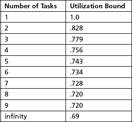
The RMA approach to scheduling tasks uses a utilization bound theorem to determine schedulability. Using this theorem, a set of n independent periodic tasks scheduled by the rate monotonic algorithm will always meet its deadlines, for all task phasings, if the total utilization of the task set is lower than the bound given in Table 8.4. This table shows the utilization bound for several examples of task numbers.
This theory is a worst case approximation. For a randomly chosen group of tasks, it has been shown that the likely upper bound is 88%. The special case where all periods are harmonic has an upper bound of 100%. The algorithm is stable in conditions where there is a transient overload. In this case, there is a subset of the total number of tasks, namely those with the highest priorities that will still meet their deadlines.
A schedulable example
As a simple example of the utilization bound theorem, assume the following tasks:
The total utilization for this task set is .2 + .2 + .3 = .7. Since this is less than the 0.779 utilization bound for this task set, all deadlines will be met.
A two-task example that can’t be scheduled
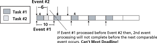
Consider the simple example of one task executing in a system as shown in Figure 8.16. This example shows a task with an execution interval of 10 (the scheduler invokes this task with a period of ten) and an execution time of 4 (ignore the time units for the time being).
If a second task is added to the system, will the system still be schedulable? As shown in Figure 8.17, a second task of period 6 with an execution time of 3 is added to the system. If task 1 is given a higher priority than task 2, then task 2 will not execute until tasks 1 completes (assuming worst case task phasings which in these examples implies that all of the tasks become ready to run at the same time). As shown in the figure, task 2 starting after task 1 completes will not finish executing before its period expires, and the system is not schedulable.
Now assume that we switch the priorities of the two tasks shown in Figure 8.17–8.21. Now task 2 runs at a higher priority than task 1. Task 1 will run after task 2 completes. This scenario is shown in Figure 8.18. In this scenario, both tasks are allowed to run to completion without interruption. In this case, task 1, which is running at a lower priority than task 2, will not complete before task 2 must run again. The system is still not schedulable.
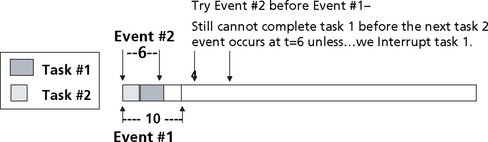
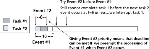
If task 1, which is running at a lower priority than task 2, is allowed to be preempted by task 1 when task 1 is ready to run, the system will become schedulable. This is shown in Figure 8.19. Task 2 runs to completion. Task 1 then begins to run. When task 2 becomes ready to run again, it interrupts task 1 and runs to completion. Task 1 then resumes execution and finishes processing.
Task sets that exceed the utilization bound but whose utilization is less than 100% require further investigation. Consider the task set below:
The total utilization is .2 + .2 + .45 = .85. This is less than the Utilization bound for a three task set, which is 0.779. This implies that the deadlines for these tasks may or may not be meet. Further analysis in this situation is required.
Completion Time Theorem
The completion time theorem says that for a set of independent periodic tasks, if each task meets its first deadline when all tasks are started at the same time, then the deadlines will be met for any combination of start times. It is necessary to check the end of the first period of a given task, as well as the end of all periods of higher priority tasks.
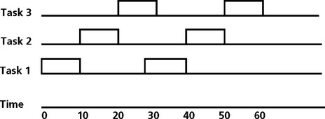
For the given task set, a time line analysis is shown in Figure 8.20.
The condition we will use for this analysis is a worst case task phasing, which implies that all three tasks become ready to run at the same time. The priorities of these tasks are assigned based on the rate monotonic scheduling approach. Task 1 has the highest priority because it has the shortest period. Task 2 has the next highest priority, followed by task 3. As shown in Figure 8.20, task 1 will meet its deadline easily, based on the fact that it is the highest priority and can pre-empt task 2 and task 3 when needed. Task 2, which executes after task 1 is complete, can also meet its deadline of 150. Task 3, the lowest priority task, must yield to task 1 and task 2 when required. Task 3 will begin execution after task 1 and task 2 have completed. At t1, task 3 is interrupted to allow task 1 to execute during its second period. When task 1 completes, task 3 resumes execution. Task 3 is interrupted again to allow task 2 to execute its second period. When task 2 completed, task 3 resumes again and finishes its processing before its period of 200. All three tasks have completed successfully (on time) based on worst case task phasings. The completion time theorem analysis has shown that the system is schedulable.
Example
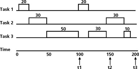
Consider the task set shown below;
The total utilization is .82. This is greater than the utilization bound for a three task set of 0.78, so the system must be analyzed further. The time line analysis for this task set is shown in Figure 8.21. In this analysis, tasks 1 and 2 make their deadline, but task 3, with a period of 50, misses its second deadline. This is an example of a timeline analysis that leads to a system that is not schedulable.
Response Time Analysis
The utilization based tests discussed earlier are a quick way to assess schedulability of a task set. The approach is not exact (if but not only if condition) and is not easily extensible to a general model.
An alternate approach is called response time analysis. In this analysis, there are two stages. The first stage is to predict the worst case response time of each task. The response time is then compared with the required deadline. This approach requires each task to be analyzed individually.
The response time analysis requires a worst case response time R, which is the time it takes a task to complete its operation after being posted. For this analysis, the same preemptive independent task model will be assumed;
where Ii is the maximum interference that task i can experience from higher priority tasks in any discrete time interval t, t + Ri. Like in the graphical analysis, the maximum interference will occur when all high priority tasks are released at the same time as task i. Therefore in the analysis we will assume all tasks are released a + t=0;
The interference from a task is computed as follows. Given a periodic task j, of higher priority than i, the number of times it is released between 0 and Ri is given by:
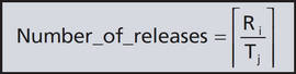
The ceiling function gives the smallest integer greater than the fractional number on which it acts. (this rounds up the fraction to an integer such that 7/4 is 2).
Each time it is released task i is delayed by its execution time Cj. This leads to the following maximum interference for a specific task.
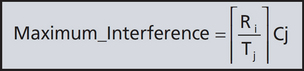
If we let hp(i) be the set of all higher priority tasks than task i, then the interference with task i can be represented as
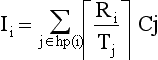
The response time is given by the fixed-point equation (note that Ri appears on both sides)
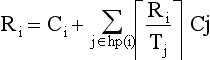
To solve the response time equation, a recurrence relationship is formed;
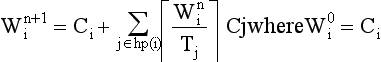
and the values of w are monotonically nondecreasing, because all numbers are positive and because of the nature of the ceiling function.
If Ri is less than the deadline than the task ti meets it deadline. If w becomes greater than the deadline, there is no solution.
Example
A second example of the response time calculation is demonstrated using the following task set:
Again, using the response time equation yields the following;
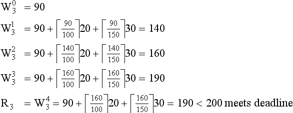
Example
One final example is now given. Consider the following task set:
As shown below, this task set fails the response time test and the system is not schedulable under all worst case conditions.
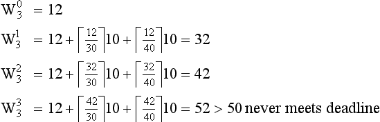
Hardware interrupts provide an effective means of notifying the application of the occurrence of external events. Interrupts are also used for sporadic I/O activities. The amount of time to service an interrupt varies based on the source of the interrupt. Interrupt handling in most processors, including DSPs, is divided into two steps; the immediate interrupt service and the scheduled interrupt service. The immediate interrupt service is executed at an interrupt priority level. The number of interrupt priority levels depends on the hardware. The TMS320C55 DSP family, for example, supports 32 interrupts with predefined priorities. All interrupt priority levels are higher than all task priorities. These interrupts are also higher in priority than the priority at which the scheduler executes as shown in Figure 8.22.
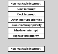
The total delay to service a DSP interrupt is the time the processor takes to complete the current instruction, do the necessary chores, and jump to the trap handler and interrupt dispatcher part of the kernel. The kernel must then disable external interrupts.
There may also be time required to complete the immediate service routines of higher priority interrupts, if any. The kernel must also save the context of the interrupted thread, identify the interrupting device, and get the starting address of the ISR. The sum of this time is called interrupt latency, it and it measures the responsiveness to external events via the interrupt mechanism. Many RTOSs provide the application with the ability to control when an interrupt is enabled again. The DSP can then control the rate at which external interrupts are serviced. The flow diagram to service a maskable and nonmaskable interrupt in the TMS320C55 DSP is shown in Figure 8.23.
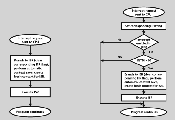
Interrupt Flow in a TMS320C55 DSP
The second part of interrupt handling in a DSP is called the scheduled interrupt service. This is another service routine invoked to complete interrupt handling. This part of interrupt processing is typically pre-emptible (unless interrupts are specifically turned off by the DSP during this time).
Context Switch Overhead
In a task based system, it takes a finite amount of time for the RTOS scheduler to switch from one running thread to a different running thread. This delay is referred to as context switch overhead.
The worst case impact of context switching a task is two scheduling actions, one when the task begins to execute and one when the task completes. In calculating the utilization bound for a task, the context switch overhead must be taken into account. This will be referred to as CS in the equation below and represent the round-trip context switch time from one task to another.
The objective of a real-time system system builder is to keep 2*CS a small fraction of the task execution time T1 (the smallest period of all tasks in the system).
Analyzing More Complex Systems
Until now, the model used to determine the schedulability of tasks has been fairly simple:
• All tasks are periodic, with known periods.
• All tasks have a deadline equal to their period.
• Rate monotonic priority assignment.
• All tasks are completely independent of each other.
• Preemptive scheduling strategy.
• Application has a fixed set of priorities (static).
In reality, there are many examples of aperiodic as well as periodic events in realtime systems. An aperiodic task is assumed to execute once within some period Ta, which represents the minimum interarrival time of the event which activates the task. The CPU time Ca is the execution time caused by a single event. The utilization time is then a worst case utilization time and can be much less than the actual. From a schedulability analysis viewpoint, an aperiodic task is equivalent to a periodic task whose period is equal to Ta and whose execution time is Ca.
An aperiodic task often needs to respond much quicker than the minimum arrival time. An example would be an error signal which interrupts very infrequently, but when it does it needs to be handled with urgency. This breaks the assumption we have made that the deadline is equal to the period. Now the deadline is less than the period. This is referred to as rate monotonic priority inversion. A rate monotonic task i can only be pre-empted once by a task with rate monotonic priority inversion as the monotonic task has a shorter period. At most the task can be blocked for the execution time of the task with the rate monotonic priority inversion. The worst case assumption is made that every lower priority task tl is blocked once by every aperiodic task with monotonic priority inversion.
Deadline Monotonic Scheduling
Deadline monotonic priority assigns the highest priorities to the jobs with the shortest deadlines:
The priorities are fixed and assigned before the application begins. It can be proven this is an optimal scheduling algorithm for deadlines less than or equal to the period T using the static scheduling model (Rate monotonic is a special case when all Di = T).
To test whether a task set is schedulable under the Deadline Monotonic policy, apply the following Deadline Monotonic scheduling to the task set;
For all jobs j(i), in the job set J {
if (R > D(i)) return unschedulable
I =Σ R / T(j) x C(j) for j = i, i-1
The Deadline Monotonic scheduling algorithm tests if all jobs will meet their deadlines under worst case conditions (critical task phasings). The worst case response time includes the delays encountered by each task by preemption from other higher priority tasks in the system. This algorithm can easily be extended to include other delay factors such as context switch times, blocking due to waiting on system resources, and other scheduler overhead and latencies:
R(i) = ((Context Switch Time(i) × 2) + Scheduler latency(i) + Blocking(i)) + C(i) + l(i)
Example: dynamic vs. static scheduling
Rate Monotonic Scheduling has shown to be optimal among static priority policies. However, some task sets that aren’t schedulable using RMS can be scheduled using dynamic strategies. An example is a task set where the deadline for completing processing is not the task period (the deadline is some time shorter than the task period). In this example, we’ll show a task set that can be scheduled under the deadline monotonic priority policy, but not under RMS.
Consider the following task set;
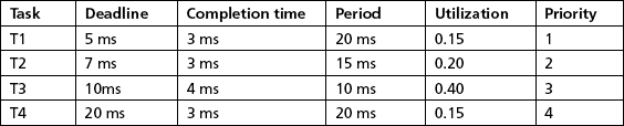
Using the Deadline Monotonic approach to scheduling, the task execution profile is shown in Figure 8.24. All tasks meet their respective deadlines using this approach.
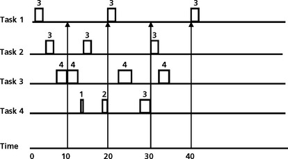
Now consider the same task set, this time prioritized using the Rate Monotonic approach to scheduling. The task priorities change using the RMA approach, as shown below:
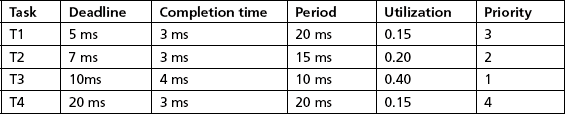
Same task set for rate monotonic scheduling
The timeline analysis using the RMA scheduling technique is shown in Figure 8.25. Notice that, using the RMA approach and the deadline constraints defined in the task set, that task 1 is now not schedulable. Although task 1 meets its period, it misses its defined deadline.
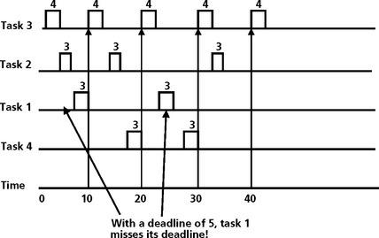
Other Dynamic Scheduling Algorithms
Other examples of dynamic scheduling algorithms include Earliest Deadline First and Least Slack Time. To successfully implement the Earliest Deadline First dynamic scheduling algorithm, the scheduler must know the deadline of the tasks. The scheduler runs the task with the closest deadline. One of he advantages of this algorithm is that the schedulable bound is 100%. Recall that, using RM scheduling, this bound approached 69% for large task sets. One of the main problems with this approach, however, is that there is no way to guarantee which tasks will fail in the case of a transient overload in the system. A transient overload is a situation where the system is temporarily overloaded beyond 100% utilization. In situations like this, it may be very important for the system to control which tasks fail and which tasks continue to exeucte. With the RM scheduling approach, the lowest priority tasks (which we know based in the a-priori assignments of task priorities) will fail while the high priority tasks will continue to exeucte. With a dynamic approach such as EDF, we do not know which tasks will fail and which ones will continue to execute.
Using the Least Slack Time algorithm, the scheduler must know the task deadline and remaining execution time. This algorithm assigns a “laxity” to each task in the system. The task with the minimum laxity is selected to execute next. The laxity term in this approach is determined by the following algorithm;
Laxity = deadline time – current time – CPU time still needed to complete processing
Laxity is basically a flexibility measure. It implies that a task can be delayed by the computed laxity time and still complete processing on time. A task that has a laxity time of zero means that the task must execute immediately or the task will fail. The least slack time approach also suffers from the limitation that there is no way to guarantee which task fails under system transient overload.
Figure 8.26 is an example of a dynamic scheduling algorithm. The three tasks t1, t2, and t3, have execution times c1, c2, and c3, and deadlines d1, d2, and d3, respectively. The EDF scheduling algorithm is used to schedule this task set. As you can see from the diagram, the tasks with the earliest deadline take priority of execution as opposed to just a static rate monotonic approach. This is illustrated in the diagram where t2 interrupts t1 to execute and t3 interrupts t2 to execute based on their respective deadlines being nearest in the future. After t3 executes, t2 finishes execution instead of t1 because if its deadline being nearer in the future than the deadline for t1.
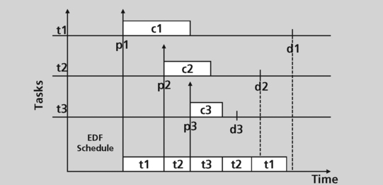
Dynamic scheduling algorithms have several advantages. If the scheduler is allowed to change the priorities of the task set during execution, you can actually get a better overall utilization (in other words a lower idle time). Dynamic algorithms also do well with aperiodic tasks. Calculations of periodicity are not required to determine the priority.
There are some disadvantages to dynamic scheduling algorithms. Dynamic scheduling algorithms such as EDF also require the scheduler to know the period of each task, which may or may not be known. Dynamic scheduling algorithms also have a higher cost of evaluation during run time. Given the extra work that must be done in the scheduler in real-time, the task switch time could be longer adding to the latency of the system. Finally, dynamic scheduling algorithms cannot accurately control which tasks will be missed during system overload conditions. In static scheduling approaches, the lower priority tasks will be the ones that may not execute during overload conditions. But in dynamically scheduled systems, this is more unpredictable.
Scheduling with Task Synchronization
Independent tasks have been assumed so far, but this is very limiting. Task interaction is common in almost all applications. Task synchronization requirements introduce a new set of potential problems. Consider the following scenario; A task enters a critical section (it needs exclusive use of a resource such as IO devices or data structures). A higher priority task preempts and wants to use the same resource. The high priority task is then blocked until the lower priority task completes. Because the low priority task could be blocked by other higher priority tasks, this is unbounded. This example of a higher-priority task having to wait for a lower-priority task is call priority inversion.
Example: priority inversion
An example of priority inversion is shown in Figure 8.27. Tasklow begins executing and requires the use of a critical section. While in the critical section, a higher priority task, Taskh preempts the lower priority task and begins its execution. During execution, this task requires the use of the same critical resource. Since the resource is already owned by the lower priority task, Taskh must block waiting on the lower priority task to release the resource. Tasklow resumes execution only to be pre-empted by a medium priority task Taskmed. Taskmed does not require the use of the same critical resource and executed to completion. Tasklow resumes execution, finishes the use of the critical resource and is immediately (actually on the next scheduling interval) pre-empted by the higher priority task which executed its critical resource, completes execution and relinquishes control back to the lower priority task to complete. Priority inversion occurs while the higher priority task is waiting for the lower priority task to release the critical resource.
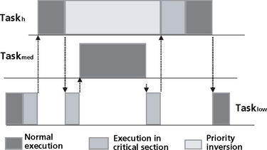
This type of priority inversion can be unbounded. The example showed a medium priority task pre-empting a lower priority task executing in a critical section and running to completion because the task did not require use of the critical resource. If there are many medium priority tasks that do not require the critical resource, they can all pre-empt the lower priority task (while the high priority task is still blocked) and execute to completion. The amount of time the high priority task may have to wait in scenarios likes this can become unbounded (Figure 8.28).
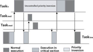
Priority inheritance protocol
There are several approaches to bound the amount of priority inversion that can exist in a task based system. One approach is a protocol called the priority inheritance protocol. If a task p is suspended waiting for a task q to undertake some computation then the priority of q becomes equal to the priority of p. Using the priority inheritance protocol, the priority assigned to tasks is dynamic as opposed to static. This protocol should not be restricted to a single step. If task L4 is waiting for L3, but L3 is waiting for L2, then L2 as well as L3 would be given L4’s priority. This implies that the run-time dispatcher has to handle tasks that are often changing priorities. This results in ineffective priority queues. The net result is that the dispatcher may be better off making the scheduling decisions at the time of action.
Example: priority inheritance
An example of PIP is shown in Figure 8.29. The same basic scenario applies. Tasklow begins executing and requires the use of a critical section. While in the critical section, a higher priority task, Taskh preempts the lower priority task and begins its execution. During execution this task requires the use of the same critical resource. Since the resource is already owned by the lower priority task, Taskh must block waiting on the lower priority task to release the resource. Tasklow resumes execution but with a new priority, one equal to the priority of Taskh!. This higher priority prevents Taskmed from pre-empting Tasklow. Tasklow runs to the end of the critical section and is then preempted by Taskh which runs to completion. Tasklow’s priority is reset to the old priority level. This allows Taskmed to pre-empt Tasklow when Taskh completes execution and, in turn will run to completion. Tasklow is then allowed to finish processing.
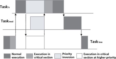
Computing a priority inheritance bound
If a task has m critical sections that can lead to it being blocked by lower-priority tasks, then the maximum number of times it can be blocked is m. If there are only n (n<m) lower priority tasks then the maximum number of times it can be blocked is n. The worst case time a task can be blocked can therefore be calculated by summing the execution time of the critical sections of all the lower priority tasks that could be used by it or tasks with the same or higher priority (that sum is referred to as Bi in the equation below).
The response time calculation with blocking is now defined as;
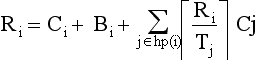
This formulation is now “if” but not “only if,” since the blockage factor can be pessimistic. For example if all tasks are periodic with the same period, no preemption will take place although the blockage calculation will result in a positive number.
Priority ceiling protocols
Priority ceiling protocols (PCP) are more complex than the simple priority inheritance protocol but have a number of advantages. Using a PCP, a high-priority task can be blocked at most once during its execution by a lower-priority task. Chains of blocks are prevented. (Task 1 being blocked by Task 2 being blocked by Task 3). Using PCP, deadlocks are prevented. Mutual exclusive access to resources is ensured.
With PCP, each shared resource has a priority ceiling which is defined as the priority of the highest priority task that can ever access that shared resource. Using PCP a task runs at its original priority when it is outside a critical section. A task can lock a shared resource only if its priority is strictly higher than the priority ceilings of all shared resources currently locked by other tasks. Otherwise, the task must block. An interesting side effect to using PCP is that a task may not be able to lock a resource, even if it is available.
The PCP has the very useful property that a task can be blocked for at most the duration of one critical section of any lower priority task. This bounds the amount of priority inversion possible.
Using the priority ceiling protocol, each task in the system has a static default priority. Each resource also has a static ceiling value defined. This is the maximum priority of the tasks that use it. Each task in the system has a dynamic priority that is the maximum of its own static priority and the ceiling values of any resources it has locked. Using the PCP protocol, a task can suffer a block only at the beginning of its execution. Once a task starts running all resources it needs must be free. If this were not the case, then some other task would have an equal or higher priority and the beginning task would not begin.
Using the priority ceiling protocol, a task can be at most interrupted by one blockage. The worst case time a task can be blocked Bi can therefore be calculated by determining the execution time of the critical sections of the longest of the lower priority tasks that could be used by it or tasks with the same or higher priority. Otherwise the response time calculation is the same.
Example: priority ceiling
An example of the priority ceiling protocol is shown in Figure 8.30. Tasklow begins execution and enters a critical section. A high priority task, Taskh, preempts Tasklow and executes until it gets to the critical section which is locked by Tasklow. At this point, control is passed to Tasklow to execute its critical section, but at a higher priority. Any attempts by medium priority tasks to pre-empt Tasklow are not allowed because of the higher priority on Tasklow and the critical resource. The amount of priority inversion experienced by Taskh is limited to the amount of time Tasklow takes to complete execution of its critical section. No other task is allowed to run before Taskh completes.
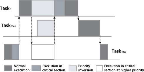
Summary
Many DSP RTOS’s (and most commercial RTOS’s in general) use static scheduling algorithms because they are simple to implement, easy to understand and support, and have a rich set of analysis techniques to draw from. DSP software developers can use Rate Monotonic Analysis to determine if the system task set is schedulable or not. If it is not schedulable, the analysis can be used to determine if there are any shared resource blocking issues which can be used to re-design the system task set and resource requirements and is especially useful for a first cut feasibility review. Most existing commercial RTOSs such as VxWorks, VRTX, and DSP RTOS’s such as DSP/BIOS use Rate Monotonic Scheduling, with some form of priority inheritance or priority ceiling protocol to limit resource blocking and priority inversion. Despite the effectiveness of this approach, DSP software developers must be aware of the limitations of static scheduling, which include inefficient handling of nonperiodic processing and nonharmonic periods, as well as the requirement of allocation of resources based on worst case estimates.
References
Dijkstra, E.W. Solution of a problem in concurrent programming control. Communications of the ACM. September 1965;9(8):569.
Knuth, Donald, E. Addition comments on a problem in concurrent programming control. Communications of the ACM. May 1966;5(9):321–322.
http://dspvillage.ti.com/docs/toolssoftwarehome.jhtml
The, Andy, Dart, David W. Texas Instruments applications report SPRA697. How to Get Started With DSP/BIOS II. October, 2000.
Liu, Jane, Hall, Prentice. Real-time Systems. 2000.
Buttazzo, Giorgio. Hard Real-time Computing Systems; Predictable scheduling Algorithms and Applications. Kluwer Academic Publishers, 1997.
Wechsler, Karl. DSP/BIOS developers conference. Designing with DSP/BIOS 2. 2001.
1An example is the interrupt latency (that is time from interrupt to task run). This has to be compatible with the application requirements and has to be predictable. This value depends on the number of simultaneous pending interrupts. For every system call, this value would be the maximum time to process the interrupt. The interrupt latency should be predictable and independent from the number of objects in the system. Another example of an important measure is the maximum time the RTOS and drivers mask the interrupts.
2Tasks are not always periodic. Tasks that are not periodic are called aperiodic. Examples of aperiodic tasks include operator requests, emergency message arrivals, threshold crossing notifications, keyboard presses, mouse movements, and detection of incoming objects.
3Disabling interrupts on multiprocessors can be time-consuming, as the message is passed to all processors.
4The restriction of no communication or synchronization may appear to be unrealistic, but there are techniques for dealing with this that will be discussed later.
5Any more and you are exceeding the capacity of the CPU. Are you asking for more computing power than you have? If so, forget it!