
Statistical Foundations of Quantitative Risk and Cost Analysis

Learning Objectives
By the end of this chapter, you will be able to:
• Define the Law of Large Numbers and the concepts of statistics and probability that derive from it.
• Explain the difference between probability and odds, and understand the roles each plays in risk decision-making.
• Apply basic rules of probability, including joint probability and union.
• Prepare a distribution of outcomes and recognize types of normal distributions (wide, narrow) and when a distribution is not normal.
• Define the three measures of central tendency (mean, median, and mode) and calculate the standard deviation of a normal distribution.
• Estimate the probability of a given outcome based on its distance from the mean as measured in standard deviations.
• Recognize that a range of distributions may apply to a given risk analysis situation.
Estimated timing for this chapter:
| Reading | 55 minutes |
| Exercises | 40 minutes |
| Review Questions | 10 minutes |
| Total Time | 1 hour 45 minutes |
QUANTITATIVE RISK AND COST ANALYSIS FUNDAMENTALS
Quantitative risk analysis, as previously noted, is the process of numerically analyzing the effect of identified risks on overall project objectives. As the name “quantitative” implies, the key word in this definition is “numerically.” Quantitative risk analysis is classical risk analysis, the probability-based tools developed to assess risk in financial instruments such as insurance. As such, it’s a fundamental part of cost analysis under conditions of uncertainty.
Quantitative risk analysis tools are normally applied to risks that our previous risk analysis has shown to be significant. Quantitative risk analysis can also be used to provide a probabilistic analysis of the likelihood of the project meeting its cost and time objectives.
The “numerical” aspect of quantitative risk analysis rests on a foundation of probability and statistics. Not everyone who has responsibility for risk and cost analysis has a background in the mathematical disciplines of probability and statistics, but some of the basic ideas from those disciplines are essential knowledge for moving ahead in this course. In this chapter, we will explain the basic concepts of statistics and probability as they apply to our topic.
If this is something you already know well, feel free to skim this chapter and move forward. If statistics wasn’t your best subject in school, or it’s been a long time since you studied it, this chapter is for you. The more serious you want to be about formal risk management, the more knowledge of these subjects you will need, so we strongly encourage further study. If you decided to skip our review on your first reading and subsequently discovered that some of the later concepts in this book don’t quite compute, welcome back.
A Statistic
There’s no evidence that the Soviet leader Joseph Stalin actually ever made a statement frequently attributed to him: “One death is a tragedy; a million deaths is a statistic.” In discussing classical risk management, the reported stalin quotation does, however, reveal an essential truth: you can’t divine a trend or tendency from a single incident.
Stalin, for example, died at the age of 74 of (apparently) natural causes. What does that tell us about the average life span (or common causes of death) in the Soviet Union at that time? Obviously, not much. What if instead we gather information on the age at death and cause of death for a million people living in the Soviet Union at that time? Well, now we really do have a statistic—sort of. Actually, it’s just a big pile of information, but it can be analyzed. The mathematical tools we use to organize and interpret the data are known as statistics.
Depending on the amount and quality of data and the depth of our analysis, there’s all sort of information to be gleaned here. If we measure the age at death of those who die next year (and know the cause of death), we can see if there’s been a change, and if so, how big it is, whether it’s a trend, and in which categories and in which directions the trend seems to be moving.
The same tools measure what we do about it. If we implement a Five-year Plan and want to know how well it’s working, we can compare the actual outcomes to the previous trend. Are we doing significantly better than we would have otherwise? The same? Worse?
As our pile of statistics grows and the quality and depth of our analysis improves, we can give answers with greater confidence. What statistics can’t tell us is the individual case: how long is Soviet citizen imya Rek going to live?
The Law of Large Numbers
The Law of Large Numbers (LLN) is a principle of probability theory. It argues that the larger the sample population or number of trials, the more likely that the actual probability will converge with the theoretical one. Roll a die a single time, and you don’t get a distribution, but an absolute value. Roll the die six times, and the actual results could be all over the map, with three of one number and one of another. Roll the die 100 times, and the likelihood increases that the resulting distribution will look like the theoretical one. (In this case, it wouldn’t be a normal distribution, but a completely flat one, because the probability of getting each individual answer is exactly the same, 1/6.)
Roll the die 1,000,000 times, and the chance the actual distribution will look like the theoretical one approaches certainty. That still doesn’t mean you’ll get identical results for each number rolled, of course. In 1,000,000 trials, a 1/6 probability you should get 166,666.667 rolls of one, but of course that’s impossible. You can roll a one 166,666 times or 166,667 times, but you can’t roll a fractional result. And, as we learned in the last chapter, we still expect some random variation. If the final results only diverge 0.1% from theoretical probability, a difference of 300 between the number of rolls of one and the number of rolls of two would be utterly insignificant.
Probability, Odds, and Throwing Dice
So far, we’ve assessed the probability of a risk event using qualitative methods—which is to say, we’ve made educated guesses, but haven’t done the math. Now, let’s look at the mathematical discipline of probability.
A science of probability didn’t get started until relatively recently in human history, and it’s arguably one of the foundations of our modern economic civilization. As we’ve seen, just about any possible decision carries with it some degree of risk. Being able to quantify the risk is fundamental to deciding to price and respond to it.
We owe the beginnings of our understanding of the mechanics of probability to a 16th century physician and compulsive gambler named Girolamo Cardano, who first articulated the basic concepts of probability in a book titled Liber de Ludo Aleae, or A Book on Games of Chance. (Benjamin, 533-544) He first conceived of expressing probability as a fraction.
This self-study course follows a long tradition of illustrating probability through gambling. Gambling provides us with an untainted theoretical environment with which to study risk. We know the odds; we know the rules; we understand the mechanics of the game. We can measure our expected loss before we put the first coin in a slot machine.
Of course, some people consistently win at gambling. These people are known as casino owners. They are able to win consistently because they apply the rules of probability with great precision to design games that provide a constant, measurable edge to the house.
Theoretical versus Actual
It’s important to keep in mind that outside a casino, it’s different.
• You often don’t know the real probability, certainty not with any precision.
• You may not know all the rules of the game, or all the factors that might affect the outcome.
• You don’t necessarily know that everyone is honest. Casinos seldom cheat because they don’t need to; the power to set the odds is more than enough. This is not always the case.
• Some situations have a likelihood and impact of an upside that is far greater than any downside risk: they are risks worth taking.
• Risks are often linked to each other in ways that aren’t obvious. Variables aren’t always independent.
• Your choices matter. Approximately 80% of small businesses fail within five years of opening. A small number of known causes account for the vast majority of failures; if you avoid those mistakes, your odds of success are dramatically higher.
For all these reasons, theoretical probability doesn’t always line up with actual probability.
Probability
A probability is expressed as a fraction: the number of desired outcomes divided by the number of possible outcomes.
There are six possible outcomes if your throw a six-sided die: one, two, three, four, five, or six. If you want to know the probability of rolling a three, three is one outcome out of six possible outcomes. Therefore, the probability of rolling a three is 1/6 (0.167, or a little less than 17%).
By the same token, in a deck of 52 cards with four aces, the chance of drawing an ace at random is 4/52 (1/13, 0.077, or a little less than 8%).
Odds
Odds measure the ratio of desired to undesired outcomes, as opposed to total outcomes. The probability of rolling a three on a six-sided die is 1/6, but the odds of rolling a three are only 1/5: one desired outcome compared to five undesired outcomes.
Imagine a game in which Player A will win $6 whenever a one is rolled, and Player B will win $6 whenever any number except a one is rolled. To balance the game so that both Player A and Player B have an equal chance of victory, you can adjust the financial stakes according to the odds: Player A bets $1 each round and Player B bets $5 each round (making up the total pot of $6). Over time, both players should end up with the same amount of money.
Basic Probabilities with One Six-Sided Die
| Roll | Probability | Odds |
| 1 | 1/6 | 1/5 |
| 2 | 1/6 | 1/5 |
| 3 | 1/6 | 1/5 |
| 4 | 1/6 | 1/5 |
| 5 | 1/6 | 1/5 |
| 6 | 1/6 | 1/5 |
BASIC RULES OF PROBABILITY
We now have two definitions: the probability of an event is the ratio of the number of times a given result occurs divided by the total number of possibilities. There is one chance in six of rolling a three on a six-sided die.
The odds of an event is the ratio of the number of times a given result occurs divided by the number of times the event does not occur. The odds of rolling a three on a six-sided die are one in five.
Exhibit 5-1 lists probabilities and odds for rolling a single die.
If you roll a six-sided die twice in a row, the outcome range becomes more complex. What is the probability and odds of rolling two threes in a row? Exhibit 5-2 lists the possible outcomes from rolling twice.
 xhibit 5-2
Basic Probabilities Rolling One Die Twice
| First Roll | Second Roll |
| 1 | 1 |
| 1 | 2 |
| 1 | 3 |
| 1 | 4 |
| 1 | 5 |
| 1 | 6 |
| 2 | 1 |
| 2 | 2 |
| 2 | 3 |
| 2 | 4 |
| 2 | 5 |
| 2 | 6 |
| 3 | 1 |
| 3 | 2 |
| 3 | 3 |
| 3 | 4 |
| 3 | 5 |
| 3 | 6 |
| 4 | 1 |
| 4 | 2 |
| 4 | 3 |
| 4 | 4 |
| 4 | 5 |
| 4 | 6 |
| 5 | 1 |
| 5 | 2 |
| 5 | 3 |
| 5 | 4 |
| 5 | 5 |
| 5 | 6 |
| 6 | 1 |
| 6 | 2 |
| 6 | 3 |
| 6 | 4 |
| 6 | 5 |
| 6 | 6 |
Rolling two threes in a row, as you can see, comes up one time out of 36 possibilities. The probability is 1/36; the odds, accordingly, are 1/35.
Of course, listing every possible outcome quickly gets tedious, so mathematicians quickly found an easier way to do it. As we already know, the probability of rolling a three on a single die roll is 1/6. The probability of doing it a second time is also 1/6. Multiply the numbers together and you get 1/36, the same answer as if you had counted them by hand. This is one of the rules of mathematical probability.
Like other branches of mathematics, probability has its own symbols and terms. Exhibit 5-3 lists common examples.
Probability Practice
Imagine you are rolling a single six-sided die. Write your answers as fractions. What are the probability and the odds that you will:
| Probability | Odds | ||
| a. | Roll a 4? | _______ | _______ |
| b. | Roll a 2? | _______ | _______ |
| c. | Not roll a 4 or a 2? | _______ | _______ |
Now imagine that you roll two six-sided dice. What are the probability and odds that you will:
| a. | Roll two 4s? | _______ | _______ |
| b. | Roll a 4 and then a 2? | _______ | _______ |
| c. | Roll a 4 after having already rolled a 2? | _______ | _______ |
| d. | Roll a 4 on at least one die? | _______ | _______ |
| e. | Not roll a 4 on at least one die? | _______ | _______ |
xhibit 5-3
Mathematical Descriptions of Probability
DISTRIBUTION
In our dice example, probabilities are distributed equally. The chance of rolling a three is equal to the chance of rolling a four, or indeed of any other number. If we roll two dice and add the numbers together, however, the picture changes, as shown in Exhibit 5-4.
xhibit 5-4
Sum of Two Dice
xhibit 5-5
Distribution of Outcomes Rolling Two Dice
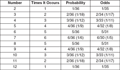
As before, there are 36 possible outcomes for rolling two dice. Notice some numbers appear more than once, and some more than others. The probability of a given roll varies, as shown in Exhibit 5-5.
Notice that a roll of 7 has the greatest likelihood (6/36, or 1/6), and rolls of 2 or 12 are least likely (1/36). Of course, the odds of not rolling a seven are still 30 in 36 (5/6), so “most likely” doesn’t automatically imply that it is in fact likely to happen. It’s simply more likely than the other possible outcomes.
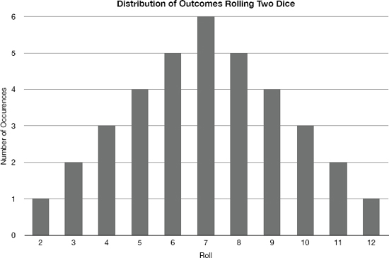
We can visualize the information by displaying it as a graph, shown in Exhibit 5-6.
NORMAL DISTRIBUTION
Exhibit 5-6 is an example of a triangular distribution, with the highest value as the mean, and a steady march downward at both ends.
As the number of data points grows larger, this kind of figure often becomes curve-shaped, the famous “bell curve” known as the normal distribution. It’s called the normal distribution not because it’s superior to other distributions, but because it occurs very often in practice. (There’s a mathematical concept known as the central limit theorem that explains why. The entry in the glossary provides a link to more information if you’re interested, but it’s not necessary for the course.)
xhibit 5-6
Normal Distribution
As we’ve established, theoretical probability doesn’t automatically equal real-world probability. Let’s imagine we roll the dice 108 (36 × 3) times. Exhibit 5-6 suggests that we should expect 18 (6 × 3) rolls of seven. If the actual tally listed 19 occurrences of seven, however, we wouldn’t be surprised, or think the dice were loaded. In a different set of 108 rolls, the actual number of sevens might be 16, or 21, and no one would think of this as strange.
Occasionally, less probable outcomes will show up. If we keep rolling long enough, we may encounter a case in which the number of sevens rolled jumps to a large number like 30, or another case in which seven shows up only 11 times.
The more extreme the result, the more we start to suspect that non-random factors are at work. Our basic probability rules say that if we have already rolled sevens 107 times in a row, the probability of rolling a seven on the 108th try would be the same as it ever was: 6/36, or one chance in six. But the chance that will happen honestly is a little less than one chance in ten followed by 85 zeros. Far more probable is that you’re playing with loaded dice. In that case, of course, the probability of rolling a seven on the 108th roll is what it’s been all along: 100%.
In other words, if the actual number is pretty close to the theoretical number, we are inclined to think the variation is random. If the actual number varies a lot, we start to regard the difference as significant. There’s usually a reason for a significant difference. Finding and managing reasons for such differences is a lot of what risk management and cost analysis is all about.
Common sense is often enough to identify significant differences, but it can also be misleading. A host of cognitive biases (Dobson, Random Jottings 6, 2011) distort our understanding and judgment when it comes to risk. Probability and statistics provide tools to help you measure and define significance in objective ways. In a normal distribution, we are interested in measures of central tendency, which provide information about the data at hand.
Measures of Central Tendency: Mean, Median, and Mode
Two statisticians shot at a target. One missed to the right, the other to the left. “On average,” the first statistician said, “we hit it.” Of course, a statistician knows that the average is not necessarily the most meaningful measure.
The average, or mean, of a group of numbers is easy to find. You add up the numbers and divide by the number of entries. To find the average of $1, $5, $7, and $9, start by adding $1+$5+$6+$9=$20, and divide the result by four, the number of items in the list: $20/4=$5. The average is $5. If we say, “They have about $5 apiece,” that gives a reasonable picture of the relative wealth of the group.
As in the case of the target-shooting statisticians, the average is not always the most useful number. If an imaginary country has three citizens, one of whom makes $1 million and the other two make $1 apiece, the average per capita income is $333,334. If we say, “They make about $333,334 a year,” however, we’re obscuring the fact that two-thirds of the citizens are starving. The high average income number doesn’t help us see the full picture.
We can add the median to the discussion. The median splits the range in the middle, so that half the values are above it and half below it. In the case of $1, $5, $7, and $9, the median is $6, because two numbers are below the median and two are above it. The mean is $5; the median is $6. When the median and mean are this close, either number reflects the relative wealth in a useful fashion.
In the case of $1, $1, and $1,000,000, the median is $1. There’s one number above and one number below. In the case of $1, $1, and $1,000,000, notice that the mean is dramatically greater than the median. The median income reveals the extreme poverty in our imaginary country, but now it obscures the fact that there is an extreme wealth difference on the right side of the income scale. Identifying both mean and median provides a more complete insight into the data.
The mode is the number that occurs most often. In the first instance, each number only occurs once. But in the second example, the mode is $1: it occurs twice, whereas $1,000,000 only occurs once. When the mode is close to the mean and median, any of the numbers convey a similar impression. If the mode is somewhere else, then there may be a reason for the unusual spike.
These three are known as measures of central tendency. In other words, they tell us what the middle of the distribution looks like. In some cases, the three measures are close together or identical; in other cases, the three measures can be dramatically different.
Normal and Other Distributions
In a normal distribution, values tend to cluster around the center, with fewer incidents at the extremes of the range. If you’re trying to find out if an observed difference is actually significant, you want to analyze its distribution.
Let’s imagine we have a big pile of six-sided dice, and we suspect—but don’t actually know—that some of them are loaded so that sevens will always result. Testing the dice with physical means will break them, which we don’t want. Fortunately, we can also test them using probability.
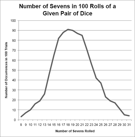
So, we design a dice-rolling machine, and feed the dice in two at a time. The machine rolls each pair 100 times, and counts the number of times a seven comes up. By the time we finish, we record data on 1000 different pairs. Let’s first imagine that we get the results shown in Exhibit 5-7.
In analyzing the distribution in Exhibit 5-7, the number of sevens rolled goes from a low of 8 to a high of 31. The majority of times the results appear pretty close to 18, which is, as you’ll recall, the expected outcome for 108 rolls, and there are only a few cases of extreme results on both ends. It’s not perfectly textbook smooth, but that’s because it’s actual probability rather than theoretical. The slight irregularities in the shape don’t provide a reason to suggest anything fishy about the dice.
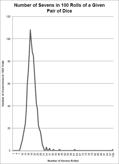
Now let’s imagine that we got very different results instead, as shown in Exhibit 5-8.
How should we interpret this distribution? For one thing, the range of outcomes is now dramatically skewed to the right. That is, there are more out-liers on the right side of the range—including one case of 100 sevens. We know immediately that at least two dice are loaded, and we want to look at the other pairs that are implicated in extremely large numbers of sevens.
But did we catch them all? We could rerun the test to find out. Does the new distribution look more like Exhibit 5-7 or Exhibit 5-8? if we see the normal distribution emerge, we suspect that we got them all. If the distribution continues to be lopsided, we need to keep looking.
In our thought experiment, the differences were so obvious that common sense was sufficient to tell the difference. But sometimes common sense can mislead, or the differences between distributions are subtle. Here’s how to do it with math.
Standard Deviation
The standard deviation is the mathematical measurement of the variance in a given normal distribution. It tells us whether the range is spread out or bunched up, and it tells us whether an observed difference is within the normal wobble or whether it rises to the level of statistical significance.
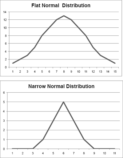
The standard deviation is represented by the Greek character σ, the little sigma. (The big sigma, ∑, normally represents “sum.”) Standard deviation measures the degree to which a normal distribution is bunched up or spread out. Let’s look at two more normal distributions. Exhibit 5-9 shows two normal distributions. The top one is a “flat” normal distribution, meaning the numbers are spread out over a wide range. On the right is a “narrow” normal distribution, meaning the numbers are bunched together in a comparatively narrow range. (As you can see from its shape, this particular example may be better described as a triangular distribution.)
Standard Deviation
![]()
σ = Standard Deviation
∑ = Sum total of what follows
d2 = The square of the deviation from the mean for each case
N = Total number of cases
√ = Square root
The standard deviation calculates how far away a number has to be from the median before it becomes significant, suggesting a real difference as opposed to natural random variation. Exhibit 5-10 provides the formula.
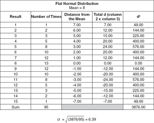
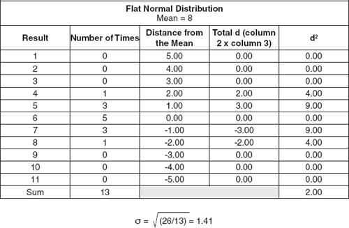
Now, let’s compare the standard deviations of the two figures. We’ll create a spreadsheet to make the math easier, as shown in Exhibit 5-11.
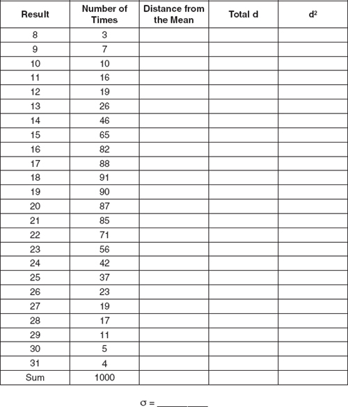
 Exercise 5-2
Calculate a Standard Deviation
In this exercise, you’ll calculate the standard deviation of the normal distribution from Exhibit 5-7. While you can do it by hand or with a calculator if you wish, we recommend using a spreadsheet program for speed and accuracy.
![]()
What’s the value of knowing the standard deviation? Well, if the difference between the actual probability and the theoretical probability is within a standard deviation (plus or minus) of the mean, then it’s not considered statistically significant.
Imagine that the sales in your department increase by $25,000 over the previous month. The question is whether that $25,000 is significant or if it’s just random. If the standard deviation is, say, $10,000, then $25,000 is a real increase in sales. But if instead the standard deviation is $100,000, then a given month’s variation of $25,000 is within the expected normal range—nothing to write home about.
Percent of Cases within 1, 2, and 3 Standard Deviations in a Normal Distribution
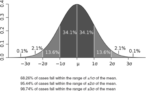
CREDIT: Standard deviation diagram, based on an original graph by Jeremy Kemp, 2005. Licensed under the Creative Commons Attribution 2.5 Generic license; downloaded from Wikimedia Commons on 11 January 2011.
We divide the range into thirds, covering one, two, and three standard deviations from the mean. Each range has an associated probability, shown in Exhibit 5-12.
In any normal distribution the farther the distance from the mean of any given variable as measured in standard deviations, the more significant.
This, by the way, is where the name “Six Sigma,” referring to the quality discipline, comes from. If errors are so rare they happen only with 6σ frequency, then they’re very rare indeed, working out to somewhere around one error per one million operations.
OTHER TYPES OF DISTRIBUTIONS
Normal distributions are commonly found in nature, but they’re far from the only kind. An exhaustive list is beyond our scope, but some other distributions include:
• Binomial distribution
• Degenerate distribution
• Discrete uniform distribution
• Hypergeometric distribution
• Extended negative binomial distribution
• Geometric distribution
• Logarithmic distribution
• Parabolic fractal distribution
• Continuous uniform distribution
• Triangular distribution
• Chi-square distribution
• Pareto distribution
You can find a list of probability distribution functions and illustrations of what they look like by searching “list of probability distributions” on Wikipedia.
Different types of distributions suggest different ideas about how to interpret the data. Although normal distributions are very common, it’s not a good idea to assume that any distribution of outcomes will automatically fall into that pattern.

Many standard tools of risk management apply concepts from probability and statistics. Probability rests on the idea of the Law of Large Numbers, the idea that the larger the sample population or number of trials, the more likely that actual probability will converge with theoretical probability. We often cannot predict the outcome of one single case, but the Law of Large Numbers allows us to predict the range of likely outcomes of many cases.
If the measure of a risk is the probability of its occurrence times the impact if it does occur, how do you figure out the probability? Probability is defined as the ratio of the number of desired outcomes to the number of total outcomes. The odds are slightly different: the ratio of the number of desired outcomes to the number of undesired outcomes. Theoretical probability is different from real probability. Flipping a coin 100 times will probably not result in exactly 50 heads and exactly 50 tails. If the number of heads is slightly greater or less, it’s no big deal. If, however, you’ve just flipped 99 heads in a row, at some point you’re likely to start assuming the coin is rigged.
The chance that both Event A and Event B will happen is measured by multiplying the probability of Event A times the probability of Event B. The probability that Event A or Event B will happen is measured by adding the probability of Event A to the probability of Event B. The probability that Event A will happen if Event B happens is measured by multiplying the probabilities of Events A and B and dividing the result by the probability of Event B.
When you combine multiple independent variables (for example, by rolling two dice instead of one), you get a distribution of outcomes. Measures of central tendency help illustrate the nature of a particular distribution. The most common measures are the mean, the median, and the mode. In a normal distribution, all three values tend to be close to the center.
Normal distributions can be wide or narrow, depending on the range. The standard deviation measures the width of the distribution, and thus helps reveal whether a particular result is merely random variation or potentially significant. Most results (roughly two-thirds) tend to fall within one standard deviation (plus or minus) of the mean of a normal distribution. The greater the distance from the mean, as measured in standard deviations, the more likely it is that a given event is statistically significant.
In addition to normal distributions, there are many other sorts of distributions. Each provides the opportunity for insight, which is why it is such an important topic in risk and cost analysis.
 Review Questions
1. What are the odds of getting three heads in a row on three flips of a coin?
(a) 1/7
(b) 1/6
(c) 1/8
(d) 1/3
1. (a)
2. If a particular result is three standard deviations from the mean in a normal distribution, it should be considered:
(a) proof that something’s wrong.
(b) statistically significant.
(c) normal.
(d) evidence that the distribution is not normal.
2. (b)
3. In a normal distribution, what percent of the results tend to fall within one standard deviation from the mean?
(a) over 95%
(b) 50%
(c) All of them
(d) About 2/3
3. (d)
4. Three measures of central tendency are the mean, the median, and the mode. The mode is defined as the:
(a) arithmetic average.
(b) square of the distance from the mean.
(c) most commonly occurring number.
(d) point that divides the range evenly.
4. (c)
5. The probability of rolling two sixes in a row with a single six-sided die is:
(a) 1/36.
(b) 1/35.
(c) 2/6.
(d) 6/36.
5. (a)