
Quantitative Schedule Analysis Tools

Learning Objectives
By the end of this chapter, you will be able to:
• Apply sensitivity analysis to project schedule issues.
• Use the tools of network diagramming and critical path analysis to construct a network diagram from a list of tasks, perform a forward and backward pass on a network diagram, identify the critical path in a network diagram, and calculate total float and free float in noncritical activities.
• Describe the three types of schedule risk.
• Create a three-point estimate for a work package with uncertain duration.
• Calculate a PERT time using a three-point estimate and determine the standard deviation for a work package and for a path using the PERT method.
• Establish a confidence level for achieving a given finish date given a PERT analysis.
• Describe the process used by a Monte Carlo simulation program for project risk management.
Estimated timing for this chapter:
| Reading | 50 minutes |
| Exercises | 1 hour 45 minutes |
| Review Questions | 10 minutes |
| Total Time | 2 hours 45 minutes |
SENSITIVITY ANALYSIS FOR SCHEDULING ISSUES
Sensitivity analysis works for time as well as for cost. We’ve been talking about cost so far, so let’s use a schedule example. We’re putting a swimming pool in our back yard. We’ve built some safety into our schedule. According to the plan, we are scheduled to finish four days ahead of the pool party.
One task in our project is called “Dig hole.” Another task is “Pour concrete.” Obviously, we can’t pour the concrete until after we’ve dug the hole. If pouring the concrete runs late, the anticipated finish of the project also goes late by the same amount. “Dig hole,” clearly, is at risk of taking longer than the scheduled time. What’s the effect on the project deadline if it does go late, say by one day? At first glance, the answer appears to be none. We have, after all, four days of total margin. One day isn’t a big deal. (At least not for the schedule. It might affect cost, especially if we’re paying people by the hour to dig the hole.)
What if we’re contracting out the pouring of the concrete? Now, it’s a different story. If the concrete truck is scheduled to pull up bright and early Tuesday morning, and the hole is only half-done, our problem suddenly balloons. It’s not just one day any more. Depending on how busy the contractor is, that one-day delay in digging the hole might cost us a week or more until we can get that concrete poured—and pretty much everything else will come to a screeching halt.
Earlier, we classified costs as either deterministic or probabilistic, depending on whether they were fixed and known. We can apply the same categories when we think about time. If you sign up for a three-day workshop, the three days are deterministic. You can put them in your schedule. The seminar won’t take two days or four days. The time-span is fixed and known.
This self-study sourcebook contains time estimates as well, based on known metrics for reading speed and length of time to complete exercises. But these estimates are probabilistic, because they are based on averages. Your mileage, as they say, may differ.
SCHEDULE RISK ANALYSIS
The technique of network diagramming enables you to display a project schedule graphically. This has numerous advantages, but for our purposes, we are concerned with network diagramming as it applies to risk management.
Time, as we all know, is money. The discipline of quantitative risk analysis must consider schedule issues as well as actual dollar costs. The length of time it takes to do the work often affects the cost, especially when people are paid by the hour. In addition, the consequences of meeting or failing to meet a deadline can be in some cases quite substantial.
The discipline of project management has long wrestled with the problem of managing uncertainty, with the first major breakthrough coming in 1957, when the U.S. Navy’s Polaris Special Projects Office and consultants from (then) Booz Allen Hamilton developed a special statistical approach to scheduling when the durations of activities were probabilistic.
The Polaris Evaluation and Review Technique helped manage what was at the time the most complex engineering project ever attempted. The “Polaris” gave way to “Program,” and the Program Evaluation and Review Technique became known as PERT. More or less at the same time, the DuPont Corporation, working with Remington Rand, developed the Critical Path Method, commonly called CPM. Both tools involve a method called network diagramming The technique of network diagramming enables you to display a project schedule graphically. This has numerous advantages, but for our purposes, we are concerned with network diagramming and schedule development as it applies to risk management.
SCHEDULE DEVELOPMENT
Two scheduling tools are common in project management: the Gantt chart, which is essentially a bar graph over a calendar; and the network diagram, which shows the sequence in which activities will be performed. For small-and medium-sized projects, the Gantt chart is the most common and easiest scheduling tool; for very large projects, the network diagram is more appropriate. Our risk management discussion will focus on network diagramming; for information on Gantt charts, consult a standard project management reference book.
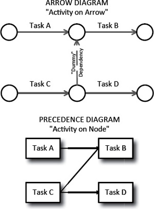
In the 1950s, the preferred technique for network diagramming was the activity on arrow method, also known as arrow diagramming. Today, virtually all project management practitioners use the precedence diagramming method (PDM), also called activity on node, which we will use throughout this section. Exhibit 8-1 shows the difference between the two techniques.
NETWORK DIAGRAMMING AND CRITICAL PATH ANALYSIS
A network diagram resembles a computer flow chart. For our purposes, the easiest way to build a network diagram is to use sticky notes. Each note will list one of the work packages or tasks to be performed. We’ll put the notes in the order in which we’ll do the work, and draw connecting arrows to show the workflow. Exhibit 8-2 shows a formal example created by computer software, but ours will be a bit more casual.
The first step is to create a “Start” milestone for your project. A milestone is a work package that has zero duration and no associated work or resource consumption. In other words, a milestone is simply a signpost. Traditionally, a milestone on a Gantt chart (but not a network diagram) is represented by a diamond. Sometimes it makes it easier to read if you turn a sticky note 45° to indicate that a given work package is a milestone.
Next, lay out the subsequent work packages in the order they are to be performed. Activities can be dependent (following a predecessor activity) or parallel (performed at the same time as other project activities. Dependent activities are sometimes required by the logic of the work (i.e., you can’t conduct a beta test of the training unless the training materials have been developed), and are sometimes driven by available resources or other factors (for example, the same person can develop the workbook and the exercises, but not at the same time. If no particular order is demanded by logic, you can choose whichever order you prefer).
 xhibit 8-1
Arrow vs. Node
Both diagrams represent the same relationships: Task B is dependent on Tasks A and C; Task D is dependent only on Task C. The “dummy” dependency in the arrow diagram shows the extra dependency relationship.
When all activities have been placed and connecting lines drawn, create a “Finish” milestone. Connect all unlinked activities to Finish so that every work package has at least one predecessor and at least one dependent activity—don’t leave any orphaned work packages.
Normally, more than one sequence of activities is possible. The correct order for your project is the one that represents how you and your team plan to approach this project. Exhibit 8-2 shows a sample network diagram.
Here’s how to read the network diagram in Exhibit 8-2. Task A is a milestone and serves as the start of the project. Both tasks B and C are dependent on the start milestone. Task D is dependent on both tasks B and C; task E is dependent only on task C. Task F is dependent on task D; task G is dependent on both tasks D and E. Task H, the finish milestone, is dependent on both tasks F and G.
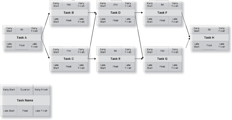
Network Diagram
This network diagram reflects the order in which work packages will be performed. Note that estimated durations have been assigned to each activity.
Forward and Backward Pass
So, how long will the project take? With dependency relationships crossing from top to bottom and back again, the answer takes a little bit of calculation. You need to find the longest path (called the critical path) through the project network to determine the length of the project. If you use project management software, it will determine the critical path for you automatically. To calculate the critical path manually, you must perform a forward pass followed by a backward pass.
Forward Pass
The forward pass calculates the early start and early finish for each activity. The final number in the forward pass calculation is the planned duration of the project. Exhibit 8-3 shows the forward pass.
Starting in the upper-left corner of the first work package, you enter a zero, which represents the start of business of the first day of the project. Add the task duration to the start, and write that number in the upper-right corner. In task A, the early start (0) is added to the duration (0) to get the early finish (0+0=0). Copy the early finish number into the connected Tasks B and C, and add the respective durations (0+15=15 and 0+11=11).
Task E, you’ll note, is dependent only on Task C, and can start on day 11. Task D, however, is dependent on both Tasks B and C. Because Task D cannot begin until both predecessor tasks are complete, it takes the larger of the two early finish dates, or day 15. Similarly, Task G takes the larger of the early finish dates of its two predecessors, Tasks D and E. At the end of the forward pass you know the duration of the project. However, you aren’t done yet.
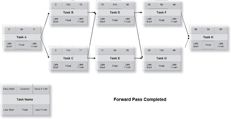
Backward Pass
If we want the project to finish within its allotted 50 days, we will now calculate the late finish and late start of each activity, shown in Exhibit 8-4. The late finish is the latest an activity can be completed while still achieving the overall deadline. The late start is the late finish minus the task duration.
Tasks F and G can both finish as late as day 48. Task F can therefore begin as late as day 40, while Task G cannot begin any later than day 36. Task D must finish in time to allow both Tasks F and G to finish no later than day 50. This means that the lower of the two late start numbers (36 in this case) is the late finish of Task D. The backward pass must end in zero when you reach the beginning of the project.
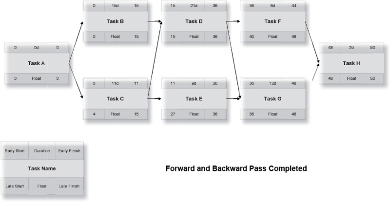
Critical Path and Float
Earlier, we said that the purpose of the forward and backward pass was to find the longest path through the project, which we call the critical path.
In our swimming pool example we differentiated between what happens if we pour the concrete ourselves (the delay is day-for-day) and if we have a scheduled date with a contractor (the delay is until the next available date in the contractor’s schedule, which could potentially be weeks).
Backward Pass
The backward pass calculates the late finish and late start of each activity, showing the latest any activity can be performed while achieving the original deadline.
Let’s go back to Exhibit 8-4 and take a look at Tasks A, B, C, and D. Notice the following:
1. Tasks B and C can’t begin until Task A is complete.
2. Task D can’t begin until Tasks B and C are complete.
3. Task B is scheduled to take 15 days.
4. Task C is scheduled to take 11 days.
If Task B takes longer than 15 days, Task D can’t start on time. However, if Task C takes longer than 11 days (and no more than 15 days), Task D’s start time is unaffected. Task C can be as many as four days late with no effect on the project schedule!
In project management, a task that can’t be late without affecting the deadline is called critical. If there’s extra time, as in the case of Task C, it’s noncritical. The extra time is called float or slack. (We’ll use “float” in this book, but either term is acceptable.) To understand and manage schedule risk, you have to manage the critical path and the available float.
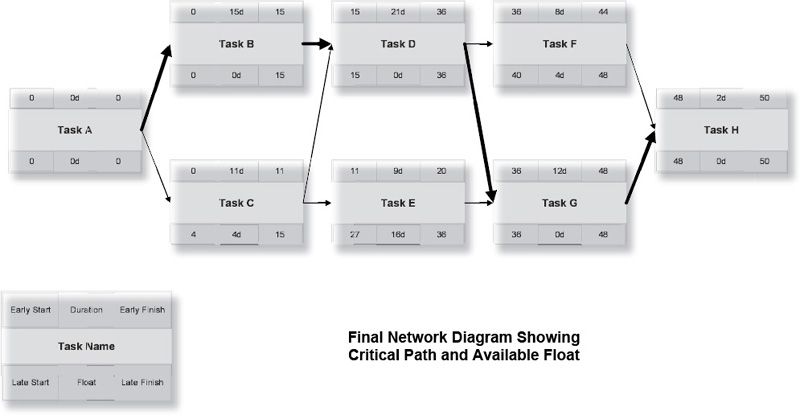
The critical path, as shown in Exhibit 8-5, is the longest path through the network. On the critical path, there is no difference between the early start (or finish) and the late start (or finish) of each activity. In other words, any delay of a critical path activity immediately introduces the danger of a late project. If a task is noncritical, it has float (also called slack), the amount of time the task can be late before the deadline is affected.
Mathematically, a task is critical if there is no difference between the early start (or finish) and the late start (or finish). If the late start (or finish) is greater than the early start (or finish), the difference is called total float. A task can have delay equal to its total float without affecting the project’s deadline. Free float is the amount of delay before the task forces a delay in any subsequent activity (whether or not it’s critical); float that is not free is shared with other activities.
Exhibit 8-5 shows the critical path and available total float.
Notice that task C can start as early as day 0 or as late as day 4. It has four days of total float (extra time before lateness jeopardizes the project deadline). However, if Task C uses any of its float, the float available for Task E is reduced because Task E will no longer start on Day 11. The float is shared, not free. The float in Tasks E and F, however, is free float, because no other task is affected if those activities use their available float.
Identify Critical Path and Float
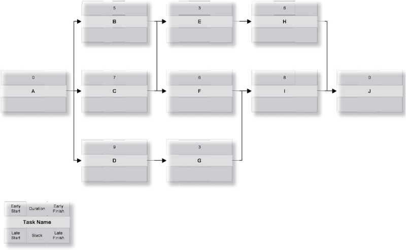
Perform a forward and backward pass on the figure above. Determine the Critical Path and identify available float.
Types of Schedule Risk
Risk to the schedule comes in three forms, illustrated in Exhibit 8-6.
• Task Duration Risk. The risk a task will take longer than the time scheduled.
• Path Duration Risk. The risk that a sequence of dependent tasks will take longer than the total time scheduled.
• Convergence Risk. The risk that at least one predecessor of a task with multiple predecessors will take longer than the time scheduled.
If there’s a specific risk to the schedule, then you normally develop a specific response. If being late digging the hole could lead to project disaster, then it makes sense to allow more time for digging the hole, or to acquire more resources with which to do it quickly.
Sometimes, the problem is simply uncertainty. When tasks involve creativity and judgment, it’s often not possible to assign an exact time in a meaningful way. You know how long it will take to teach a three-day class, but when it comes to writing the course for that three-day class, you’ll be a lot less precise. “It’ll take three or four weeks” is often about as honest an estimate as you’re able to provide. Throwing extra people at the job won’t necessarily help. Occasionally, it’ll make things worse.
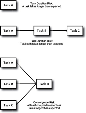
If you have unavoidable uncertainty about how long individual activities in your project will take (task duration risk), you automatically end up with path duration risk for any path that includes those tasks, and you have convergence risk whenever one of those paths links up with any other path in your project.
How can you figure out how long the project will take when you can’t be sure how long key tasks will take? Once again, you’re into the realm of probability.
THREE-POINT ESTIMATING TECHNIQUES
We have to dig a hole every time we put in a new swimming pool, but yards are different. Weather interferes. Equipment breaks down. The time it takes to dig a hole varies. Over time, we would naturally expect the hole-digging times to form a distribution, whether normal, triangular, or some other type, just as we’ve seen in cost analysis.
Historical Times for a Common Task
| Hole | Duration |
| 1 | 3 days |
| 2 | 4 days |
| 3 | 2 days |
| 4 | 2 days |
| 5 | 5 days |
| 6 | 3 days |
| 7 | 4 days |
| 8 | 3 days |
| 9 | 4 days |
| 10 | 3 days |
| Optimistic (Best Case) | 2 days |
| Most Likely (Median) | 3 days |
| Pessimistic (Worst Case) | 5 days |
We can define the schedule distribution with a three-point estimate. Instead of using a single number as our estimate, we use three: the optimistic (best case) time, the pessimistic (worst case) time, and the most likely estimate (either the mean or the median). Figure 8-7 provides some historical times for digging that hole that we can use in creating a three-point estimate.
The range is between 2 and 5 days, and the median is 3 days, and now we have our three estimates.
You can create three estimates even if you don’t have historical records to draw on. In fact, a lot of people find that it’s actually easier to create three estimates than one, because you can use different assumptions to make them.
PERT Formulas
T(e) = (T(o) + 4 T(m) + T(p)) / 6
σ = (T(p) – T(o)) / 6
where:
T(e) = PERT Estimate
T(o) = Optimistic Estimate
T(m) = Most Likely Estimate
T(p) = Pessimistic Estimate
σ = Standard Deviation of T(e) for a Single Task
Program Evaluation and Review Technique (PERT)
Three-point estimating was developed as part of the PERT method. PERT is a comprehensive approach to project management, but we’re only concerned here with a particular portion of PERT that applies to risk analysis.
Let’s say we have a large network diagram with hundreds (or thousands) of tasks, many of which have a high level of uncertainty in the estimates, so we’ve created a three-point estimate for each of those tasks. The question now is what to do with those three numbers. Clearly, it’s unwise to plan as if we’ll get the optimistic time on every task, and it’s excessive to believe that all tasks will have a pessimistic outcome. We could use the most likely numbers, but that can be quite misleading as well.
PERT applies two formulas to those numbers, both shown in Exhibit 8-8. The first formula creates the PERT estimate, a weighted average of the three numbers. The second formula is how PERT calculates the standard deviation. In this context, the standard deviation is a measure of the degree of schedule risk (uncertainty) in the particular estimate.
By this measure, the PERT estimate (T(e)) for our “dig hole” activity is (2 + (4 × 3) + 5) / 6 = 19 / 6 = 3.16 days, and the standard deviation (σ) is (5 – 2) / 6 = 0.5 days. In Exercise 8-2, create the other PERT estimates for the tasks in our swimming pool project and enter them in the network diagram provided.
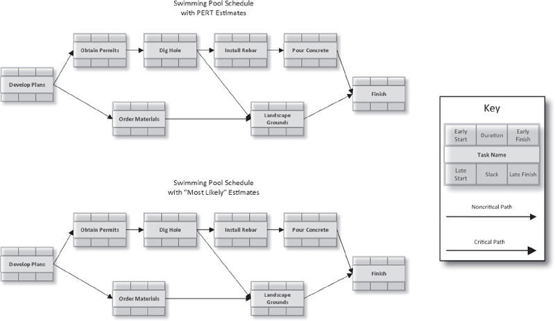
Scheduling With PERT Estimates
Step 1. Calculate the PERT estimate (T(e)) and standard deviation (σ) for each of the tasks in the swimming pool project using the information below. Round PERT estimates to the nearest whole day.
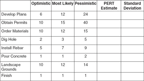
Step 2. Complete the network diagrams below. In the first diagram, use the PERT estimates for each task. For comparison, use the “most likely” estimates in the second diagram.
Confidence Levels
| Standard Deviation | Confidence Level |
| 0σ | 50% |
| 1σ | 68.27% |
| 1.28σ | 80% |
| 1.64σ | 90% |
| 1.96σ | 95% |
| 2σ | 95.45% |
| 2.58σ | 99.00% |
| 2.81σ | 99.50% |
| 3σ | 99.73% |
| 3.29σ | 99.90% |
| 4σ | 99.99% |
Confidence Levels and the Standard Deviation
When we priced the risk for our insurance policy, we added a standard deviation to the base price of the risk to increase safety. Similarly, the standard deviation serves as a tool for what we might call “scientific padding”—risk-adjusting your schedule by allowing extra time to compensate for known uncertainty.
Using the standard deviation, we can determine a confidence level for the schedule, a measurement of how likely it is that the project will finish on or before a given date. Exhibit 8-9 provides a table showing the confidence levels associated with specific standard deviations.
In Exercise 8-2, we found that the “most likely” schedule took 43 days, and the PERT estimated schedule took 47. The confidence level for the 47-day estimate is 50%—that is, there’s only a 50% chance that the project will finish on or before Day 47. What if we wanted to be 80% certain the project would finish on time? According to Exhibit 8-9, we need to add 1.28 σ to the estimate.
Now all we have to do is find the standard deviation for the project. To do that, take the standard deviations for each of the tasks on the critical path. Square them, add up the numbers, and take the square root of the sum (also called the root sum square). The answer is the standard deviation for the project. Multiply that by the confidence level desired, and that’s how much extra time you need to allow.
 Exercise 8-3
Calculating Standard Deviation for a Path or Network
Using the table from Step 1 of Exercise 8-2, square the standard deviations of the tasks on the critical path, sum them, and take the square root of the sum. Now, using the information in Exhibit 8-9, calculate the project duration at the following levels of confidence:
| 80% confidence | = | ___________ |
| 90% confidence | = | ___________ |
| 95% confidence | = | ___________ |
Advantages and Disadvantages of PERT
As you may have noticed, the PERT formula for calculating the standard deviation doesn’t resemble the formula you learned in Chapter 5. In fact, from a statistics perspective, there are a lot of problems with PERT.
There’s a reason for this. When PERT was first developed in the late 1950s, computing horsepower was limited and expensive. It was simply impossible to perform a full analysis of a network containing tens of thousands of work packages in a reasonable timeframe. The brilliant minds behind PERT resorted to shortcuts. They made assumptions about the distribution and standard deviation (known as “back-fitting the curve”) and developed formulas that were cheaper and easier to compute based on those assumptions.
PERT estimates are very useful and have been applied successfully on major projects, but you should always treat a PERT analysis with caution. It provides a useful yardstick to measure schedule risk, but its answer tends to be far from precise. PERT is particularly subject to convergence risk, meaning that the PERT estimate tends to provide an optimistic view of how long the project will take to complete.
PERT works best when the project has a dominant single critical path; it is much less reliable when the relationships among paths and tasks are highly complex. PERT is an important element in the history of project schedule risk management, and the fundamental three-point estimating technique is still used, but most operating project managers who need to perform schedule risk analysis have switched from PERT to the Monte Carlo simulation technique.
Monte Carlo Simulation
While the PERT method attempts to measure schedule risk by calculation, the Monte Carlo simulation measures schedule risk by massive simulation, run by specialized software. Monte Carlo simulation programs for project management are available as plug-ins for common project management programs such as Microsoft Project® as well as in stand-alone versions.
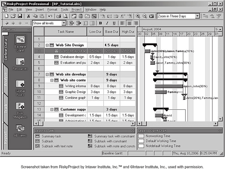
To run a Monte Carlo simulation, you first need the same three-point estimates for task durations that you would use in performing a PERT analysis. (You also need the other elements of a completed project schedule, including a list of tasks and their dependency relationships, of course.) While a standard project management software package provides space to enter a single time estimate for a task, a Monte Carlo program provides places to enter all three estimates, as shown in Exhibit 8-10.
In PERT, we used statistical tools to analyze the schedule, but a Monte Carlo simulation uses more of a “brute force” approach. The simulation pretends that we are actually managing the project. It decides how long it takes to accomplish a particular task by selecting a random number from the range provided. For our swimming pool project task “Develop Plans,” with an optimistic estimate of 6, most likely 12, and pessimistic 24, the program might choose 15 as the duration of the task for this iteration.
It then checks to see if a finish time of 15 days alters the start dates of any subsequent activities, and adjusts as necessary. Then it goes to the next task (“Order Materials”) and selects a number between 10 and 15. Let’s say it’s 11. Again, it checks to see if any start times have been moved, and then to the next task, and so on until the project ends. Perhaps the answer is 49 days this time. The program stores that number, goes back to the top, and does it again. And again, and again, and so on for 5,000 or 6,000 trials.
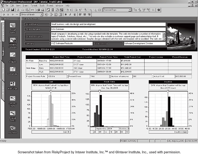
The output of the program is a distribution showing how often the project ended on a given date. Exhibit 8-11 provides an example. In this particular program, the slider on top of each histogram allows you to see the date or cost associated with any desired confidence level.
While the technique has been understood for a long time, it is only recently that the increase in computer processing speed and reduction in cost has made the technique practical.
A Monte Carlo simulation is much more robust than a PERT analysis, and normally deserves more weight in decision-making. As you can see, a Monte Carlo simulation can simulate cost as well as schedule, as long as you enter the cost data (salary costs and other expenses that vary with time spent) into the program.
Monte Carlo simulation programs are commonly available as add-ins for project management software packages. There’s a list available in the “Additional Resources” section of this book, but you should remember that software availability and features change frequently.

The tools of quantitative risk analysis extend to schedule as well as cost. Quantitative schedule analysis requires the development of a network diagram, a flow chart of the work packages and activities that make up the project.
Knowing how to develop a network diagram is fundamental to many aspects of project planning. In the most commonly used technique, known as the precedence diagramming method, work packages are represented as nodes (boxes) and connected by their dependency relationships (arrows). Once the work package durations have been estimated, you can perform a forward and backward pass (or let project management software do it for you) to reveal the critical path (the longest path through the network, equal to the project duration) and the availability of float, extra time to perform activities not on the critical path. Critical path analysis identifies which tasks must be completed on time if you are going to meet the desired end date.
Schedule risk comes in three forms:
• Task Duration Risk. The risk a task will take longer than the time scheduled.
• Path Duration Risk. The risk that a sequence of dependent tasks will take longer than the total time scheduled.
• Convergence Risk. The risk that at least one predecessor of a task with multiple predecessors will take longer than the time scheduled.
The seriousness (sensitivity) of a task duration risk is compounded by its effect on path duration risk and convergence risk.
Specific risks to the schedule require specific risk mitigation responses, but some schedule risk is simply the inherent uncertainty in knowing how long it will take to accomplish certain tasks. In that case, where estimates are highly probabilistic, project risk managers can use three-point estimates to show the range and distribution of potential outcomes.
The PERT analysis technique uses probability mechanics. The PERT time estimate is a weighted average derived from the three-point estimate. The standard deviation of the PERT estimate serves as a barometer of schedule risk. By taking the root sum square of the standard deviations of the work packages on the critical path, you can determine the confidence level that your project will achieve a given deadline.
More powerful computers have led to the rise of the Monte Carlo simulation technique, which uses a repetitive technique of iterating the schedule many times to create a distribution of completion time, dates, and costs.
 Review Questions
1. If Task B has three days of total float, which statement must be true?
(a) Task B is expected to take three days to complete.
(b) Task B is a critical task.
(c) If Task B is delayed no more than three days, the start date of no other task will be affected.
(d) If Task B is delayed no more than three days, the expected project completion date is not affected.
1. (d)
2. Three-point estimates are used in which risk analysis techniques?
(a) PERT analysis and Monte Carlo simulation
(b) Probabilistic analysis and PERT analysis
(c) Monte Carlo simulation and sensitivity analysis
(d) Probabilistic analysis and sensitivity analysis
2. (a)
3. What does a network diagram show?
(a) The sequence in which activities will be performed
(b) A bar graph of task durations over a calendar grid
(c) The breakdown and logical organization of the work structure
(d) The IT infrastructure for your project
3. (a)
4. A skilled machine operator can produce 50 widgets per hour. If the machine breaks down, the same operator can perform the necessary repairs. Which statement is true?
(a) The time to produce a given number of widgets is probabilistic; the time to fix the machine if it breaks is deterministic.
(b) The time to produce a given number of widgets is deterministic; the time to fix the machine if it breaks is probabilistic.
(c) Both times are deterministic.
(d) Both times are probabilistic.
4. (b)
5. The risk that at least one predecessor of a task with multiple predecessors will take longer than the time scheduled is known as:
(a) task duration risk.
(b) convergence risk.
(c) predecessor risk.
(d) path duration risk.