Chapter Fifteen. Radix Search
Several search methods proceed by examining the search keys one small piece at a time, rather than using full comparisons between keys at each step. These methods, called radix-search methods, operate in a manner entirely analogous to the radix-sorting methods that we discussed in Chapter 10. They are useful when the pieces of the search keys are easily accessible, and they can provide efficient solutions to a variety of practical search tasks.
We use the same abstract model that we used in Chapter 10: Depending on the context, a key may be a word (a fixed-length sequence of bytes) or a string (a variable-length sequence of bytes). We treat keys that are words as numbers represented in a base-R number system, for various values of R (the radix), and work with individual digits of the numbers. We can view C strings as variable-length numbers terminated by a special symbol so that, for both fixed- and variable-length keys, we can base all our algorithms on the abstract operation “extract the ith digit from a key,” including a convention to handle the case that the key has fewer than i digits.
The principal advantages of radix-search methods are that the methods provide reasonable worst-case performance without the complication of balanced trees; they provide an easy way to handle variable-length keys; some of them allow space savings by storing part of the key within the search structure; and they can provide fast access to data, competitive with both binary search trees and hashing. The disadvantages are that some of the methods can make inefficient use of space, and that, as with radix sorting, performance can suffer if efficient access to the bytes of the keys is not available.
First, we examine several search methods that proceed by examining the search keys 1 bit at a time, using them to travel through binary tree structures. We examine a series of methods, each one correcting a problem inherent in the previous one, culminating in an ingenious method that is useful for a variety of search applications.
Next, we examine generalizations to R-way trees. Again, we examine a series of methods, culminating in a flexible and efficient method that can support a basic symbol-table implementation and numerous extensions.
In radix search, we usually examine the most significant digits of the keys first. Many of the methods directly correspond to MSD radix-sorting methods, in the same way that BST-based search corresponds to quicksort. In particular, we shall see the analog to the linear-time sorts of Chapter 10—constant-time search methods based on the same principle.
At the end of the chapter, we consider the specific application of using radix-search structures to build indexes for large text strings. The methods that we consider provide natural solutions for this application, and help to set the stage for us to consider more advanced string-processing tasks in Part 5.
15.1 Digital Search Trees
The simplest radix-search method is based on use of digital search trees (DSTs). The search and insert algorithms are identical to binary tree search except for one difference: We branch in the tree not according to the result of the comparison between the full keys, but rather according to selected bits of the key. At the first level, the leading bit is used; at the second level, the second leading bit is used; and so on, until an external node is encountered. Program 15.1 is an implementation of search; the implementation of insert is similar. Rather than using less to compare keys, we assume that the digit function is available to access individual bits in keys. This code is virtually the same as the code for binary tree search (see Program 12.7), but has substantially different performance characteristics, as we shall see.
We saw in Chapter 10 that we need to pay particular attention to equal keys in radix sorting; the same is true in radix search. Generally, we assume in this chapter that all the key values to appear in the symbol table are distinct. We can do so without loss of generality because we can use one of the methods discussed in Section 12.1 to support applications that have records with duplicate keys. It is important to focus on distinct key values in radix search, because key values are intrinsic components of several of the data structures that we shall consider.
Figure 15.1 gives binary representations for the one-letter keys used in other figures in the chapter. Figure 15.2 gives an example of insertion into a DST; Figure 15.3 shows the process of inserting keys into an initially empty tree.

As we did in Chapter 10, we use the 5-bit binary representation of i to represent the ith letter in the alphabet, as shown here for several sample keys, for the small examples in the figures in this chapter. We consider the bits as numbered from 0 to 4, from left to right.
Figure 15.1 Binary representation of single-character keys
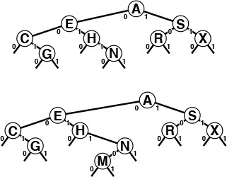
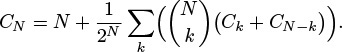
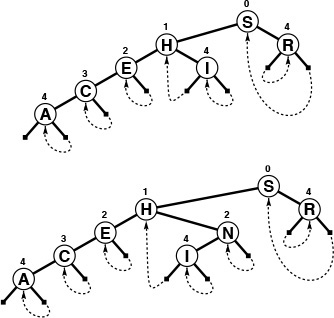
In an unsuccessful search for M = 01101 in this sample digital search tree (top), we move left at the root (since the first bit in the binary representation of the key is 0) then right (since the second bit is 1), then right, then left, to finish at the null left link below N. To insert M (bottom), we replace the null link where the search ended with a link to the new node, just as we do with BST insertion.
Figure 15.2 Digital search tree and insertion
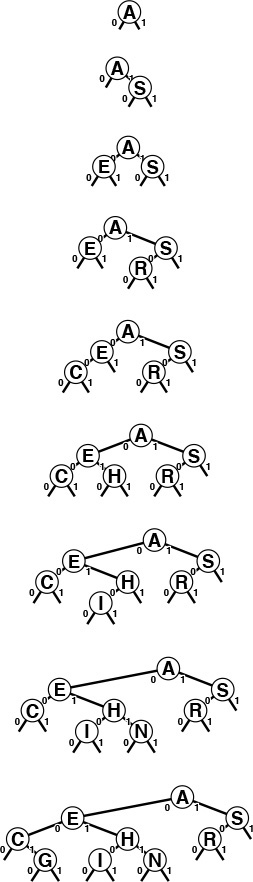
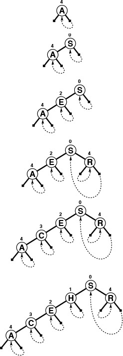
This sequence depicts the result of inserting the keys A S E R C H I N G into an initially empty digital search tree.
Figure 15.3 Digital search tree construction
The bits of the keys control search and insertion, but note that DSTs do not have the ordering property that characterizes BSTs. That is, it is not necessarily the case that nodes to the left of a given node have smaller keys or that nodes to the right have larger keys, as would be the case in a BST with distinct keys. It is true that keys on the left of a given node are smaller than keys on the right—if the node is at level k, they all agree in the first k bits, but the next bit is 0 for the keys on the left and is 1 for the keys on the right—but the node’s key could itself could be the smallest, largest, or any value in between of all the keys in that node’s subtree.
DSTs are characterized by the property that each key is somewhere along the path specified by the bits of the key (in order from left to right). This property is sufficient for the search and insert implementations in Program 15.1 to operate properly.
Suppose that the keys are words of a fixed length, all consisting of w bits. Our requirement that keys are distinct implies that N ≤ 2w, and we normally assume that N is significantly smaller than 2w, since otherwise key-indexed search (see Section 12.2) would be the appropriate algorithm to use. Many practical problems fall within this range. For example, DSTs are appropriate for a symbol table containing up to 105 records with 32-bit keys (but perhaps not as many as 106 records), or for any number of 64-bit keys. Digital tree search also works for variable-length keys; we defer considering that case in detail to Section 15.2, where we consider a number of other alternatives as well.
The worst case for trees built with digital search is much better than that for binary search trees, if the number of keys is large and the key lengths are small relative to the number of keys. The length of the longest path in a digital search tree is likely to be relatively small for many applications (for example, if the keys comprise random bits). In particular, the longest path is certainly limited by the length of the longest key; moreover, if the keys are of a fixed length, then the search time is limited by the length. Figure 15.4 illustrates this fact.
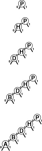
This sequence depicts the result of inserting the keys P = 10000, H = 01000, D = 00100, B = 00010, and A = 00001 into an initially empty digital search tree. The sequence of trees appears degenerate, but the path length is limited by the length of the binary representation of the keys. Except for 00000, no other 5-bit key will increase the height of the tree any further.
Figure 15.4 Digital search tree, worst case
Property 15.1 A search or insertion in a digital search tree requires about lg N comparisons on the average, and about 2 lg N comparisons in the worst case, in a tree built from N random keys. The number of comparisons is never more than the number of bits in the search key.
We can establish the stated average-case and worst-case results for random keys with an argument similar to one given for a more natural problem in the next section, so we leave this proof for an exercise there (see Exercise 15.29). It is based on the simple intuitive notion that the unseen portion of a random key should be equally likely to begin with a 0 bit as a 1 bit, so half should fall on either side of any node. Each time that we move down the tree, we use up a key bit, so no search in a digital search tree can require more comparisons than there are bits in the search key. For the typical condition where we have w-bit words and the number of keys N is far smaller than the total possible number of keys 2w, the path lengths are close to lg N, so the number of comparisons is far smaller than the number of bits in the keys for random keys. ![]()
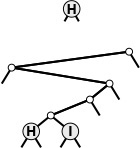
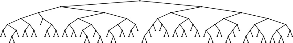
Figure 15.5 shows a large digital search tree made from random 7-bit keys. This tree is nearly perfectly balanced. DSTs are attractive in many practical applications because they provide near-optimal performance even for huge problems, with little implementation effort. For example, a digital search tree built from 32-bit keys (or four 8-bit characters) is guaranteed to require fewer than 32 comparisons, and a digital search tree built from 64-bit keys (or eight 8-bit characters) is guaranteed to require fewer than 64 comparisons, even if there are billions of keys. For large N, these guarantees are comparable to the guarantee provided by red–black trees, but are achieved with about the same implementation effort as is required for standard BSTs (which can promise only guaranteed performance proportional to N2). This feature makes the use of digital search trees an attractive alternative to use of balanced trees in practice for implementing the search and insert symbol-table functions, provided that efficient access to key bits is available.
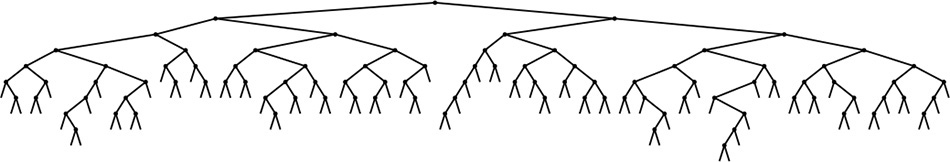
This digital search tree, built by insertion of about 200 random keys, is as well-balanced as its counterparts in Chapter 15.
Figure 15.5 Digital search tree example
Exercises
![]() 15.1 Draw the DST that results when you insert items with the keys E A S Y Q U T I O N in that order into an initially empty tree, using the binary encoding given in Figure 15.1.
15.1 Draw the DST that results when you insert items with the keys E A S Y Q U T I O N in that order into an initially empty tree, using the binary encoding given in Figure 15.1.
15.2 Give an insertion sequence for the keys A B C D E F G that results in a perfectly balanced DST that is also a valid BST.
15.3 Give an insertion sequence for the keys A B C D E F G that results in a perfectly balanced DST with the property that every node has a key smaller than those of all the nodes in its subtree.
![]() 15.4 Draw the DST that results when you insert items with the keys
15.4 Draw the DST that results when you insert items with the keys 0101-0011 00000111 00100001 01010001 11101100 00100001 10010101 01001010 in that order into an initially empty tree.
15.5 Can we keep records with duplicate keys in DSTs, in the same way that we can in BSTs? Explain your answer.
15.6 Run empirical studies to compare the height and internal path length of a DST built by insertion of N random 32-bit keys into an initially empty tree with the same measures of a standard binary search tree and a red–black tree (Chapter 13) built from the same keys, for N = 103, 104, 105, and 106.
![]() 15.7 Give a full characterization of the worst-case internal path length of a DST with N distinct w-bit keys.
15.7 Give a full characterization of the worst-case internal path length of a DST with N distinct w-bit keys.
![]() 15.8 Implement the delete operation for a DST-based symbol table.
15.8 Implement the delete operation for a DST-based symbol table.
![]() 15.9 Implement the select operation for a DST-based symbol table.
15.9 Implement the select operation for a DST-based symbol table.
![]() 15.10 Describe how you could compute the height of a DST made from a given set of keys, in linear time, without building the DST.
15.10 Describe how you could compute the height of a DST made from a given set of keys, in linear time, without building the DST.
15.2 Tries
In this section, we consider a search tree that allows us to use the bits of the keys to guide the search, in the same way that DSTs do, but that keeps the keys in the tree in order, so that we can support recursive implementations of sort and other symbol-table functions, as we did for BSTs. The idea is to store keys only at the bottom of the tree, in leaf nodes. The resulting data structure has a number of useful properties and serves as the basis for several effective search algorithms. It was first discovered by de la Briandais in 1959, and, because it is useful for retrieval, it was given the name trie by Fredkin in 1960. Ironically, in conversation, we usually pronounce this word “try-ee” or just “try,” so as to distinguish it from “tree.” For consistency with the nomenclature that we have been using, we perhaps should use the name “binary search trie,” but the term trie is universally used and understood. We consider the basic binary version in this section, an important variation in Section 15.3, and the basic multiway version and variations in Sections 15.4 and 15.5.
We can use tries for keys that are either a fixed number of bits or are variable-length bitstrings. To simplify the discussion, we start by assuming that no search key is the prefix of another. For example, this condition is satisfied when the keys are of fixed length and are distinct.
In a trie, we keep the keys in the leaves of a binary tree. Recall from Section 5.4 that a leaf in a tree is a node with no children, as distinguished from an external node, which we interpret as a null child. In a binary tree, a leaf is an internal node whose left and right links are both null. Keeping keys in leaves instead of internal nodes allows us to use the bits of the keys to guide the search, as we did with DSTs in Section 15.1, while still maintaining the basic invariant at each node that all keys whose current bit is 0 fall in the left subtree and all keys whose current bit is 1 fall in the right subtree.
Definition 15.1 A trie is a binary tree that has keys associated with each of its leaves, defined recursively as follows: The trie for an empty set of keys is a null link; the trie for a single key is a leaf containing that key; and the trie for a set of keys of cardinality greater than one is an internal node with left link referring to the trie for the keys whose initial bit is 0 and right link referring to the trie for the keys whose initial bit is 1, with the leading bit considered to be removed for the purpose of constructing the subtrees.
Each key in the trie is stored in a leaf, on the path described by the leading bit pattern of the key. Conversely, each leaf contains the only key in the trie that begins with the bits defined by the path from the root to that leaf. Null links in nodes that are not leaves correspond to leading-bit patterns that do not appear in any key in the trie. Therefore, to search for a key in a trie, we just branch according to its bits, as we did with DSTs, but we do not do comparisons at internal nodes. We start at the left of the key and the top of the trie, and take the left link if the current bit is 0 and the right link if the current bit is 1, moving one bit position to the right in the key. A search that ends on a null link is a miss; a search that ends on a leaf can be completed with one key comparison, since that node contains the only key in the trie that could be equal to the search key. Program 15.2 is an implementation of this process.
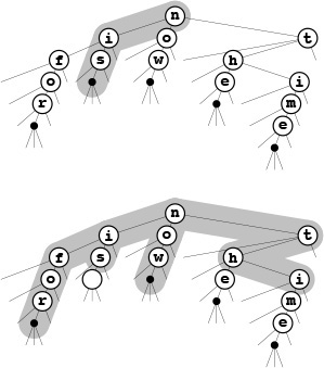
To insert a key into a trie, we first perform a search, as usual. If the search ends on a null link, we replace that link with a link to a new leaf containing the key, as usual. But if the search ends on a leaf, we need to continue down the trie, adding an internal node for every bit where the search key and the key that was found agree, ending with both keys in leaves as children of the internal node corresponding to the first bit position where they differ. Figure 15.6 gives an example of trie search and insertion; Figure 15.7 shows the process of constructing a trie by inserting keys into an initially empty trie. Program 15.3 is a full implementation of the insertion algorithm.
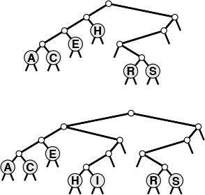
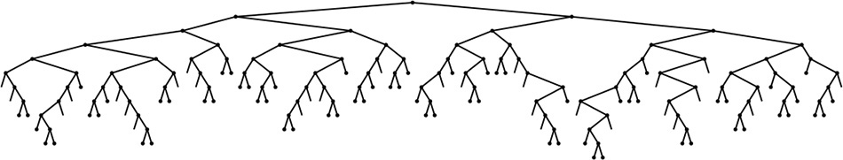
Keys in a trie are stored in leaves (nodes with both links null); null links in nodes that are not leaves correspond to bit patterns not found in any keys in the trie.
In a successful search for the key H = 01000 in this sample trie (top), we move left at the root (since the first bit in the binary representation of the key is 0), then right (since the second bit is 1), where we find H, which is the only key in the tree that begins with 01. None of the keys in the trie begin with 101 or 11; these bit patterns lead to the two null links in the trie that are in non-leaf nodes.
To insert I (bottom), we need to add three non-leaf nodes: one corresponding to 01, with a null link corresponding to 011; one corresponding to 010, with a null link corresponding to 0101; and one corresponding to 0100 with H = 01000 in a leaf on its left and I = 01001 in a leaf on its right.
Figure 15.6 Trie search and insertion
This sequence depicts the result of inserting the keys A S E R C H I N into an initially empty trie.
Figure 15.7 Trie construction
We do not access null links in leaves, and we do not store items in non-leaf nodes, so we could save space in a C implementation by using union to define nodes as being one of these two types (see Exercise 15.20). For the moment, we will take the simpler route of using the single node type that we have been using for BSTs, DSTs, and other binary tree structures, with internal nodes characterized by null keys and leaves characterized by null links, knowing that we could reclaim the space wasted because of this simplification, if desired. In Section 15.3, we will see an algorithmic improvement that avoids the need for multiple node types, and in Chapter 16, we will examine an implementation that uses union.
We now shall consider a number of basic of properties of tries, which are evident from the definition and these examples.
Property 15.2 The structure of a trie is independent of the key insertion order: There is a unique trie for any given set of distinct keys.
This fundamental fact, which we can prove by induction on the subtrees, is a distinctive feature of tries: for all the other search tree structures that we have considered, the tree that we construct depends both on the set of keys and on the order in which we insert those keys. ![]()
The left subtree of a trie has all the keys that have 0 for the leading bit; the right subtree has all the keys that have 1 for the leading bit. This property of tries leads to an immediate correspondence with radix sorting: binary trie search partitions the file in exactly the same way as does binary quicksort (see Section 10.2). This correspondence is evident when we compare the trie in Figure 15.6 with Figure 10.4, the partitioning diagram for binary quicksort (after noting that the keys are slightly different); it is analogous to the correspondence between binary tree search and quicksort that we noted in Chapter 12.
In particular, unlike DSTs, tries do have the property that keys appear in order, so we can implement the sort and select symbol-table operations in a straightforward manner (see Exercises 15.17 and 15.18). Moreover, tries are as well-balanced as DSTs.
Property 15.3 Insertion or search for a random key in a trie built from N random (distinct) bitstrings requires about lg N bit comparisons on the average. The worst-case number of bit comparisons is bounded only by the number of bits in the search key.
We need to exercise care in analyzing tries because of our insistence that the keys be distinct, or, more generally, that no key be a prefix of another. One simple model that accommodates this assumption requires the keys to be a random (infinite) sequence of bits—we take the bits that we need to build the trie.
The average-case result then comes from the following probabilistic argument. The probability that each of the N keys in a random trie differ from a random search key in at least one of the leading t bits is
Subtracting this quantity from 1 gives the probability that one of the keys in the trie matches the search key in all of the leading t bits. In other words,
is the probability that the search requires more than t bit comparisons. From elementary probabilistic analysis, the sum for t ≥ 0 of the probabilities that a random variable is > t is the average value of that random variable, so the average search cost is given by
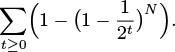
Using the elementary approximation (1 − 1/x)x ∼ e−1, we find the search cost to be approximately
The summand is extremely close to 1 for approximately lg N terms with 2t substantially smaller than N; it is extremely close to 0 for all the terms with 2t substantially greater than N; and it is somewhere between 0 and 1 for the few terms with 2t ≈ N. So the grand total is about lg N. Computing a more precise estimate of this quantity requires using extremely sophisticated mathematics (see reference section). This analysis assumes that w is sufficiently large that we never run out of bits during a search, but taking into account the true value of w will only reduce the cost.
In the worst case, we could get two keys that have a huge number of equal bits, but this event happens with vanishingly small probability. The probability that the worst-case result quoted in Property 15.3 will not hold is exponentially small (see Exercise 15.28). ![]()
Another approach to analyzing tries is to generalize the approach that we used to analyze BSTs (see Property 12.6). The probability that k keys start with a 0 bit and N − k keys start with a 1 bit is ![]() , so the external path length is described by the recurrence
, so the external path length is described by the recurrence
This recurrence is similar to the quicksort recurrence that we solved in Section 7.2, but it is much more difficult to solve. Remarkably, the solution is precisely N times the expression for the average search cost that we derived for Property 15.3 (see Exercise 15.25). Studying the recurrence itself gives insight into why tries have better balance than do BSTs: The probability is much higher that the split will be near the middle than that it will be anywhere else, so the recurrence is more like the mergesort recurrence (approximate solution N lg N) than like the quicksort recurrence (approximate solution 2N ln N).
An annoying feature of tries, and another one that distinguishes them from the other types of search trees that we have seen, is the oneway branching required when keys have bits in common. For example, keys that differ in only the final bit always require a path whose length is equal to the key length, no matter how many keys there are in the tree, as illustrated in Figure 15.8. The number of internal nodes can be somewhat larger than the number of keys.
This sequence depicts the result of inserting the keys H = 01000 and I = 01001 into an initially empty binary trie. As it is in DSTs (see Figure 15.4), the path length is limited by the length of the binary representation of the keys; as illustrated by this example, however, paths could be that long even with only two keys in the trie.
Figure 15.8 Binary trie worst case
Property 15.4 A trie built from N random w-bit keys has about N/ ln 2 ≈ 1.44N nodes on the average.
By modifying the argument for Property 15.3, we can write the expression

for the average number of nodes in an N-key trie (see Exercise 15.26). The mathematical analysis that yields the stated approximate value for this sum is much more difficult than the argument that we gave for Property 15.3, because many terms contribute values that are not 0 or 1 to the value of the sum (see reference section). ![]()
We can verify these results empirically. For example, Figure 15.9 shows a big trie, which has 44 percent more nodes than does the BST or the DST built with the same set of keys but nevertheless is well balanced, with a near-optimal search cost. Our first thought might be that the extra nodes would raise the average search cost substantially, but this suspicion is not valid—for example, we would increase the average search cost by only 1 even if we were to double the number of nodes in a balanced trie.
This trie, built by inserting about 200 random keys, is well-balanced, but has 44 percent more nodes than might otherwise be necessary, because of one-way branching. (Null links on leaves are not shown.)
Figure 15.9 Trie example
For convenience in the implementations in Programs 15.2 and 15.3, we assumed that the keys are of fixed length and are distinct, so that we could be certain that the keys would eventually distinguish themselves and that the programs could process 1 bit at a time and never run out of key bits. For convenience in the analyses in Properties 15.2 and 15.3, we implicitly assumed that the keys have an arbitrary number of bits, so that they eventually distinguish themselves except with tiny (exponentially decaying) probability. A direct off-shoot of these assumptions is that both the programs and the analyses apply when the keys are variable-length bitstrings, with a few caveats.
To use the programs as they stand for variable-length keys, we need to extend our restriction that the keys be distinct to say that no key be a prefix of another. This restriction is met automatically in some applications, as we shall see in Section 15.5. Alternatively, we could handle such keys by keeping information in internal nodes, because each prefix that might need to be handled corresponds to some internal node in the trie (see Exercise 15.30).
For sufficiently long keys comprising random bits, the average-case results of Properties 15.2 and 15.3 still hold. In the worst case, the height of a trie is still limited by the number of bits in the longest keys. This cost could be excessive if the keys are huge and perhaps have some uniformity, as might arise in encoded character data. In the next two sections, we consider methods of reducing trie costs for long keys. One way to shorten paths in tries is to collapse one-way branches into single links—we discuss an elegant and efficient way to accomplish this task in Section 15.3. Another way to shorten paths in tries is to allow more than two links per node—this approach is the subject of Section 15.4.
Exercises
![]() 15.11 Draw the trie that results when you insert items with the keys E A S Y Q U T I O N in that order into an initially empty trie.
15.11 Draw the trie that results when you insert items with the keys E A S Y Q U T I O N in that order into an initially empty trie.
15.12 What happens when you use Program 15.3 to insert a record whose key is equal to some key already in the trie?
15.13 Draw the trie that results when you insert items with the keys 0101-0011 00000111 00100001 01010001 11101100 00100001 10010101 01001010 into an initially empty trie.
15.14 Run empirical studies to compare the height, number of nodes, and internal path length of a trie built by insertion of N random 32-bit keys into an initially empty trie with the same measures of a standard binary search tree and a red–black tree (Chapter 13) built from the same keys, for N = 103, 104, 105, and 106(see Exercise 15.6).
15.15 Give a full characterization of the worst-case internal path length of a trie with N distinct w-bit keys.
![]() 15.16 Implement the delete operation for a trie-based symbol table.
15.16 Implement the delete operation for a trie-based symbol table.
![]() 15.17 Implement the select operation for a trie-based symbol table.
15.17 Implement the select operation for a trie-based symbol table.
15.18 Implement the sort operation for a trie-based symbol table.
![]() 15.19 Write a program that prints out all keys in a trie that have the same initial
15.19 Write a program that prints out all keys in a trie that have the same initial t bits as a given search key.
![]() 15.20 Use the C
15.20 Use the C union construct to develop implementations of search and insert using tries with non-leaf nodes that contain links but no items and with leaves that contain items but no links.
15.21 Modify Programs 15.3 and 15.2 to keep the search key in a machine register and to shift one bit position to access the next bit when moving down a level in the trie.
15.22 Modify Programs 15.3 and 15.2 to maintain a table of 2r tries, for a fixed constant r, and to use the first r bits of the key to index into the table and the standard algorithms with the remainder of the key on the trie accessed. This change saves about r steps unless the table has a significant number of null entries.
15.23 What value should we choose for r in Exercise 15.22, if we have N random keys (which are sufficiently long that we can assume them to be distinct)?
15.24 Write a program to compute the number of nodes in the trie corresponding to a given set of distinct fixed-length keys, by sorting them and comparing adjacent keys in the sorted list.
![]() 15.25 Prove by induction that N Σt≥0(1 – (1 – 2−t)N) is the solution to the quicksort-like recurrence that is given after Property 15.3 for the external path length in a random trie.
15.25 Prove by induction that N Σt≥0(1 – (1 – 2−t)N) is the solution to the quicksort-like recurrence that is given after Property 15.3 for the external path length in a random trie.
![]() 15.26 Derive the expression given in Property 15.4 for the average number of nodes in a random trie.
15.26 Derive the expression given in Property 15.4 for the average number of nodes in a random trie.
![]() 15.27 Write a program to compute the average number of nodes in a random trie of N nodes and print the exact value, accurate to 10− 3, for N = 103, 104, 105, and 106.
15.27 Write a program to compute the average number of nodes in a random trie of N nodes and print the exact value, accurate to 10− 3, for N = 103, 104, 105, and 106.
![]() 15.28 Prove that the height of a trie built from N random bitstrings is about 2 lg N. Hint: Consider the birthday problem (see Property 14.2).
15.28 Prove that the height of a trie built from N random bitstrings is about 2 lg N. Hint: Consider the birthday problem (see Property 14.2).
![]() 15.29 Prove that the average cost of a search in a DST built from random keys is asymptotically lg N (see Properties 15.1 and 15.2).
15.29 Prove that the average cost of a search in a DST built from random keys is asymptotically lg N (see Properties 15.1 and 15.2).
15.30 Modify Programs 15.2 and 15.3 to handle variable-length bitstrings under the sole restriction that records with duplicate keys are not kept in the data structure. Assume that bit(v, w) yields the value NULLdigit if w is greater than the length of v.
15.31 Use a trie to build a data structure that can support an existence table ADT for w-bit integers. Your program should support the initialize, insert, and search operations, where search and insert take integer arguments, and search returns NULLkey for search miss and the argument it was given for search hit.
15.3 Patricia Tries
Trie-based search as described in Section 15.2 has two inconvenient flaws. First, the one-way branching leads to the creation of extra nodes in the trie, which seem unnecessary. Second, there are two different types of nodes in the trie, and that complicates the code somewhat. In 1968, Morrison discovered a way to avoid both of these problems, in a method that he named patricia (“practical algorithm to retrieve information coded in alphanumeric”). Morrison developed his algorithm in the context of string-indexing applications of the type that we shall consider in Section 15.5, but it is equally effective as a symbol-table implementation. Like DSTs, patricia tries allow search for N keys in a tree with just N nodes; like tries, they require only about lg N bit comparisons and one full key comparison per search, and they support other ADT operations. Moreover, these performance characteristics are independent of key length, and the data structure is suitable for variable-length keys.
Starting with the standard trie data structure, we avoid one-way branching via a simple device: we put into each node the index of the bit to be tested to decide which path to take out of that node. Thus, we jump directly to the bit where a significant decision is to be made, bypassing the bit comparisons at nodes where all the keys in the subtree have the same bit value. Moreover, we avoid external nodes via another simple device: we store data in internal nodes and replace links to external nodes with links that point back upwards to the correct internal node in the trie. These two changes allow us to represent tries with binary trees comprising nodes with a key and two links (and an additional field for the index), which we call patricia tries. With patricia tries, we store keys in nodes as with DSTs, and we traverse the tree according to the bits of the search key, but we do not use the keys in the nodes on the way down the tree to control the search; we merely store them there for possible later reference, when the bottom of the tree is reached.
As hinted in the previous paragraph, it is easier to follow the mechanics of the algorithm if we first take note that we can regard standard tries and patricia tries as different representations of the same abstract trie structure. For example, the tries in Figure 15.10 and at the top in Figure 15.11, which illustrate search and insertion for patricia tries, represent the same abstract structure as do the tries in Figure 15.6. The search and insertion algorithms for patricia tries use, build, and maintain a concrete representation of the abstract trie data structure different from the search and insertion algorithms discussed in Section 15.2, but the underlying trie abstraction is the same.
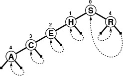
In a successful search for R = 10010 in this sample patricia trie (top), we move right (since bit 0 is 1), then left (since bit 4 is 0), which brings us to R (the only key in the tree that begins with 1***0). On the way down the tree, we check only the key bits indicated in the numbers over the nodes (and ignore the keys in the nodes). When we first reach a link that points up the tree, we compare the search key against the key in the node pointed to by the up link, since that is the only key in the tree that could be equal to the search key.
In an unsuccessful search for I = 01001, we move left at the root (since bit 0 of the key is 0), then take the right (up) link (since bit 1 is 1) and find that H (the only key in the trie that begins with 01) is not equal to I.
Figure 15.10 Patricia search
To insert I into the sample patricia trie in Figure 15.10, we add a new node to check bit 4, since H = 01000 and I = 01001 differ in only that bit (top). On a subsequent search in the trie that comes to the new node, we want to check H (left link) if bit 4 of the search key is 0; if the bit is 1 (right link), the key to check is I.
To insert N = 01110 (bottom), we add a new node in between H and I to check bit 2, since that bit distinguishes N from H and I.
Figure 15.11 Patricia-trie insertion
Program 15.4 is an implementation of the patricia-trie search algorithm. The method differs from trie search in three ways: there are no explicit null links, we test the indicated bit in the key instead of the next bit, and we end with a search key comparison at the point where we follow a link up the tree. It is easy to test whether a link points up, because the bit indices in the nodes (by definition) increase as we travel down the tree. To search, we start at the root and proceed down the tree, using the bit index in each node to tell us which bit to examine in the search key—we go right if that bit is 1, left if it is 0. The keys in the nodes are not examined at all on the way down the tree. Eventually, an upward link is encountered: each upward link points to the unique key in the tree that has the bits that would cause a search to take that link. Thus, if the key at the node pointed to by the first upward link encountered is equal to the search key, then the search is successful; otherwise, it is unsuccessful.
Figure 15.10 illustrates search in a patricia trie. For a miss due to the search taking a null link in a trie, the corresponding patricia trie search will take a course somewhat different from that of standard trie search, because the bits that correspond to one-way branching are not tested at all on the way down the trie. For a search ending at a leaf in a trie, the patricia-trie search ends up comparing against the same key as the trie search, but without examining the bits corresponding to one-way branching in the trie.
The implementation of insertion for patricia tries mirrors the two cases that arise in insertion for tries, as illustrated in Figure 15.11. As usual, we gain information on where a new key belongs from a search miss. For tries, the miss can occur either because of a null link or because of a key mismatch at a leaf. For patricia tries, we need to do more work to decide which type of insertion is needed, because we skipped the bits corresponding to one-way branching during the search. A patricia-trie search always ends with a key comparison, and this key carries the information that we need. We find the leftmost bit position where the search key and the key that terminated the search differ, then search through the tree again, comparing that bit position against the bit positions in the nodes on the search path. If we come to a node that specifies a bit position higher than the bit position that distinguishes the key sought and the key found, then we know that we skipped a bit in the patricia-trie search that would have led to a null link in the corresponding trie search, so we add a new node for testing that bit. If we never come to a node that specifies a bit position higher than the one that distinguishes the key sought and the key found, then the patricia-trie search corresponds to a trie search ending in a leaf, and we add a new node that distinguishes the search key from the key that terminated the search. We always add just one node, which references the leftmost bit that distinguishes the keys, where standard trie insertion might add multiple nodes with one-way branching before reaching that bit. That new node, besides providing the bit-discrimination that we need, will also be the node that we use to store the new item. Figure 15.12 shows the initial stages of the construction of a sample trie.
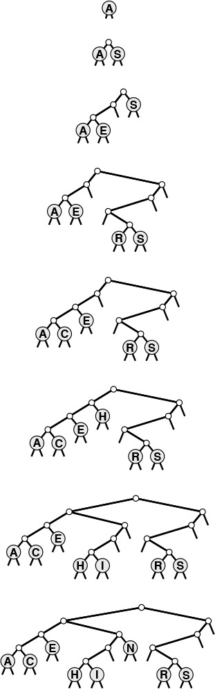
This sequence depicts the result of inserting the keys A S E R C H into an initially empty patricia trie. Figure 15.11 depicts the result of inserting I and then N into the tree at the bottom.
Figure 15.12 Patricia-trie construction
Program 15.5 is an implementation of the patricia-trie–insertion algorithm. The code follows directly from the description in the previous paragraph, with the additional observation that we view links to nodes with bit indices that are not larger than the current bit index as links to external nodes. The insertion code merely tests this property of the links, but does not have to move keys or links around at all. The upward links in patricia tries seem mysterious at first, but the decisions about which links to use when each node is inserted are surprisingly straightforward. The end result is that using one node type rather than two simplifies the code substantially.
By construction, all external nodes below a node with bit index k begin with the same k bits (otherwise, we would have created a node with bit index less than k to distinguish two of them). Therefore, we can convert a patricia trie to a standard trie by creating the appropriate internal nodes between nodes where bits are skipped and by replacing links that point up the tree with links to external nodes (see Exercise 15.47). However, Property 15.2 does not quite hold for patricia tries, because the assignment of keys to internal nodes does depend on the order in which the keys are inserted. The structure of the internal nodes is independent of the key-insertion order, but external links and the placement of the key values are not.
An important consequence of the fact that a patricia trie represents an underlying standard trie structure is that we can use a recursive inorder traversal to visit the nodes in order, as demonstrated in the implementation given in Program 15.6. We visit just the external nodes, which we identify by testing for nonincreasing bit indices.
Patricia is the quintessential radix search method: it manages to identify the bits that distinguish the search keys and to build them into a data structure (with no surplus nodes) that quickly leads from any search key to the only key in the data structure that could be equal to the search key. Figure 15.13 shows the patricia trie for the same keys used to build the trie of Figure 15.9—the patricia trie not only has 44 percent fewer nodes than the standard trie, but also is nearly perfectly balanced.
This patricia trie, built by insertion of about 200 random keys, is equivalent to the trie of Figure 15.9 with one-way branching removed. The resulting tree is nearly perfectly balanced.
Figure 15.13 Patricia-trie example
Property 15.5 Insertion or search for a random key in a patricia trie built from N random bitstrings requires about lg N bit comparisons on the average, and about 2 lg N bit comparisons in the worst case. The number of bit comparisons is never more than the length of the key.
This fact is an immediate consequence of Property 15.3, since paths in patricia tries are no longer than paths in the corresponding trie. The precise average-case analysis of patricia is difficult; it turns out that patricia involves one fewer comparison, on the average, than does a standard trie (see reference section). ![]()
Table 15.1 gives empirical data supporting the conclusion that DSTs, standard binary tries, and patricia tries have comparable performance (and that they provide search times comparable to or shorter than the balanced-tree methods of Chapter 13) when keys are integers, and certainly should be considered for symbol-table implementations even with keys that can be represented as short bitstrings, taking into account the various straightforward tradeoffs that we have noted.
These relative timings for construction and search in symbol tables with random sequences of 32-bit integers confirm that digital methods are competitive with balanced-tree methods, even for keys that are random bits. Performance differences are more remarkable when keys are long and are not necessarily random (see Table 15.2), or when careful attention is paid to making the key-bit–access code efficient (see Exercise 15.21).
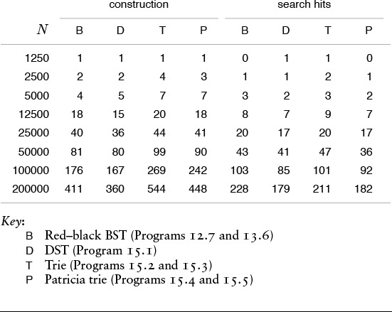
Table 15.1 Empirical study of trie implementations
Note that the search cost given in Property 15.5 does not grow with the key length. By contrast, the search cost in a standard trie typically does depend on the length of the keys—the first bit position that differs in two given keys could be arbitrarily far into the key. All the comparison-based search methods that we have considered also depend on the key length—if two keys differ in only their rightmost bit, then comparing them requires time proportional to their length. Furthermore, hashing methods always require time proportional to the key length for a search, to compute the hash function. But patricia immediately takes us to the bits that matter, and typically involves testing less than lg N of them. This effect makes patricia (or trie search with one-way branching removed) the search method of choice when the search keys are long.
For example, suppose that we have a computer that can efficiently access 8-bit bytes of data, and we have to search among millions of 1000-bit keys. Then patricia would require accessing only about 20 bytes of the search key for the search, plus one 125-byte equality comparison, whereas hashing would require accessing all 125 bytes of the search key to compute the hash function, plus a few equality comparisons, and comparison-based methods would require 20 to 30 full key comparisons. It is true that key comparisons, particularly in the early stages of a search, require only a few byte comparisons, but later stages typically involve many more bytes. We shall consider comparative performance of various methods for searching with lengthy keys again in Section 15.5.
Indeed, there needs to be no limit at all on the length of search keys for patricia. Patricia is particularly effective in applications with variable-length keys that are potentially huge, as we shall see in Section 15.5. With patricia, we generally can expect that the number of bit inspections required for a search among N records, even with huge keys, will be roughly proportional to lg N.
Exercises
15.32 What happens when you use Program 15.5 to insert a record whose key is equal to some key already in the trie?
![]() 15.33 Draw the patricia trie that results when you insert the keys E A S Y Q U T I O N in that order into an initially empty trie.
15.33 Draw the patricia trie that results when you insert the keys E A S Y Q U T I O N in that order into an initially empty trie.
![]() 15.34 Draw the patricia trie that results when you insert the keys
15.34 Draw the patricia trie that results when you insert the keys 01010011 00000111 00100001 01010001 11101100 00100001 10010101 01001010 in that order into an initially empty trie.
![]() 15.35 Draw the patricia trie that results when you insert the keys
15.35 Draw the patricia trie that results when you insert the keys 01001010 10010101 00100001 11101100 01010001 00100001 00000111 01010011 in that order into an initially empty trie.
15.36 Run empirical studies to compare the height and internal path length of a patricia trie built by insertion of N random 32-bit keys into an initially empty trie with the same measures of a standard binary search tree and a red–black tree (Chapter 13) built from the same keys, for N = 103, 104, 105, and 106(see Exercises 15.6 and 15.14).
15.37 Give a full characterization of the worst-case internal path length of a patricia trie with N distinct w-bit keys.
![]() 15.38 Implement the select operation for a patricia-based symbol table.
15.38 Implement the select operation for a patricia-based symbol table.
![]() 15.39 Implement the delete operation for a patricia-based symbol table.
15.39 Implement the delete operation for a patricia-based symbol table.
![]() 15.40 Implement the join operation for patricia-based symbol tables.
15.40 Implement the join operation for patricia-based symbol tables.
![]() 15.41 Write a program that prints out all keys in a patricia trie that have the same initial
15.41 Write a program that prints out all keys in a patricia trie that have the same initial t bits as a given search key.
15.42 Modify standard trie search and insertion (Programs 15.2 and 15.3) to eliminate one-way branching in the same manner as for patricia tries. If you have done Exercise 15.20, start with that program instead.
15.43 Modify patricia search and insertion (Programs 15.4 and 15.5) to maintain a table of 2r tries, as described in Exercise 15.22.
15.44 Show that each key in a patricia trie is on its own search path, and is therefore encountered on the way down the tree during a search operation as well as at the end.
15.45 Modify patricia search (Program 15.4) to compare keys on the way down the tree to improve search-hit performance. Run empirical studies to evaluate the effectiveness of this change (see Exercise 15.44).
15.46 Use a patricia trie to build a data structure that can support an existence table ADT for w-bit integers (see Exercise 15.31).
![]() 15.47 Write programs that convert a patricia trie to a standard trie on the same keys, and vice versa.
15.47 Write programs that convert a patricia trie to a standard trie on the same keys, and vice versa.
15.4 Multiway Tries and TSTs
For radix sorting, we found that we could get a significant improvement in speed by considering more than 1 bit at a time. The same is true for radix search: By examining r bits at a time, we can speed up the search by a factor of r. However, there is a catch that makes it necessary for us to be more careful in applying this idea than we had to be for radix sorting. The problem is that considering r bits at a time corresponds to using tree nodes with R = 2r links, and that can lead to a considerable amount of wasted space for unused links.
In the (binary) tries of Section 15.2, the nodes corresponding to key bits have two links: one for the case when the key bit is 0, and the other for the case when the key bit is 1. The appropriate generalization is to R-ary tries, where we have nodes with R links corresponding to key digits, one for each possible digit value. Keys are stored in leaves (nodes with all links null). To search in an R-way trie, we start at the root and at the leftmost key digit, and use the key digits to guide us down the tree. We go down the ith link (and move to the next digit) if the digit value is i. If we reach a leaf, it contains the only key in the trie with leading digits corresponding to the path that we have traversed, so we can compare that key with the search key to determine whether we have a search hit or a search miss. If we reach a null link, we know that we have a search miss, because that link corresponds to a leading-digit pattern not found in any keys in the trie. Figure 15.14 shows a 10-way trie that represents a sample set of decimal numbers. As we discussed in Chapter 10, numbers typically seen in practice are distinguished with relatively few trie nodes. This same effect for more general types of keys is the basis for a number of efficient search algorithms.
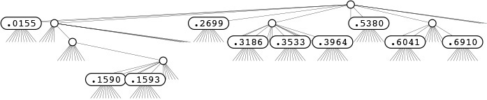
This figure depicts the trie that distinguishes the set of numbers.396465048.353336658.318693642.015583409.159369371.691004885.899854354.159072306.604144269.269971047.538069659
(see Figure 12.1). Each node has 10 links (one for each possible digit). At the root, link 0 points to the trie for keys with first digit 0 (there is only one); link 1 points to the trie for keys with first digit 1 (there are two), and so forth. None of these numbers has first digit 4, 7, 8, or 9, so those links are null. There is only one number for each of the first digits 0, 2, and 5, so there is a leaf containing the appropriate number for each of those digits. The rest of the structure is built recursively, moving one digit to the right.
Figure 15.14 R-way trie for base-10 numbers
Before doing a full symbol-table implementation with multiple node types and so forth, we begin our study of multiway tries by concentrating on the existence-table problem, where we have only keys (no records or associated information) and want to develop algorithms to insert a key into a data structure and to search the data structure to tell us whether or not a given key has been inserted. To use the same interface that we have been using for more general symbol-table implementations, we assume that Key is the same as Item and adopt the convention that the search function returns NULLitem for a search miss and the search key for a search hit. This convention simplifies the code and clearly exposes the structure of the multiway tries that we shall be considering. In Section 15.5, we shall discuss more general symbol-table implementations, including string indexing.
Definition 15.2 The existence trie corresponding to a set of keys is defined recursively as follows: The trie for an empty set of keys is a null link; and the trie for a nonempty set of keys is an internal node with links referring to the trie for each possible key digit, with the leading digit considered to be removed for the purpose of constructing the subtrees.
For simplicity, we assume in this definition that no key is the prefix of another. Typically, we enforce this restriction by ensuring that the keys are distinct and either are of fixed length or have a termination character. The point of this definition is that we can use existence tries to implement existence tables, without storing any information within the trie; the information is all implicitly defined within the trie structure. Each node has R +1 links (one for each possible character value plus one for the terminal character NULLdigit), and no other information. To search, we use the digits in the key to guide us down the trie. If we reach the link to NULLdigit at the same time that we run out of key digits, we have a search hit; otherwise we have a search miss. To insert a new key, we search until we reach a null link, then add nodes for each of the remaining characters in the key. Figure 15.15 is an example of a 27-way trie; Program 15.7 is an implementation of the basic (multiway) existence-trie search and insert procedures.
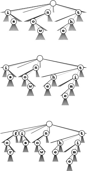
The 26-way trie for the words now, is, and the (top) has nine nodes: the root plus one for each letter. The nodes are labeled in these diagrams, but we do not use explicit node labels in the data structure, because each node label can be inferred from the position of the link to it in its parents’ link array.
To insert the key time, we branch off the existing node for t and add new nodes for i, m, and e (center); to insert the key for, we branch off the root and add new nodes for f, o, and r.
Figure 15.15 R-way existence trie search and insertion
If the keys are of fixed length and are distinct, we can dispense with the link to the terminal character and can terminate searches when we reach the key length (see Exercise 15.54). We have already seen an example of this type of trie when we used tries to describe MSD sorting for fixed-length keys (Figure 10.10).
In one sense, this pure abstract representation of the trie structure is optimal, because it can support the search operation in time proportional to the length of a key and in space proportional to the total number of characters in the key in the worst case. But the total amount of space used could be as high as nearly R links for each character, so we seek improved implementations. As we saw with binary tries, it is worthwhile to consider the pure trie structure as a particular representation of an underlying abstract structure that is a well-defined representation of our set of keys, and then to consider other representations of the same abstract structure that might lead to better performance.
Definition 15.3 A multiway trie is a multiway tree that has keys associated with each of its leaves, defined recursively as follows: The trie for an empty set of keys is a null link; the trie for a single key is a leaf containing that key; and the trie for a set of keys of cardinality greater than one is an internal node with links referring to tries for keys with each possible digit value, with the leading digit considered to be removed for the purpose of constructing the subtrees.
We assume that keys in the data structure are distinct and that no key is the prefix of another. To search in a standard multiway trie, we use the digits of the key to guide the search down the trie, with three possible outcomes. If we reach a null link, we have a search miss; if we reach a leaf containing the search key, we have a search hit; and if we reach a leaf containing a different key, we have a search miss. All leaves have R null links, so different representations for leaf nodes and non-leaf nodes are appropriate, as mentioned in Section 15.2. We consider such an implementation in Chapter 16, and we shall consider another approach to an implementation in this chapter. In either case, the analytic results from Section 15.3 generalize to tell us about the performance characteristics of standard multiway tries.
Property 15.6 Search or insertion in a standard R-ary trie built from N random bytestrings requires about logR N byte comparisons, on the average. The number of links in a such a trie is about RN/ ln R. The number of byte comparisons for search or insertion in such a trie is no more than the number of bytes in the search key.
These results generalize those in Properties 15.3 and 15.4. We can establish them by substituting R for 2 in the proofs of those properties. As we mentioned, however, extremely sophisticated mathematics is involved in the precise analysis of these quantities. ![]()
The performance characteristics listed in Property 15.6 represent an extreme example of a time–space tradeoff. On the one hand, there are a large number of unused null links—only a few nodes near the top use more than a few of their links. On the other hand, the height of a tree is small. For example, suppose that we take the typical value R = 256 and that we have N random 64-bit keys. Property 15.6 tells us that a search will take (lg N)/8 character comparisons (8 at most) and that we will use fewer than 47N links. If plenty of space is available, this method provides an extremely efficient alternative. We could cut the search cost to 4 character comparisons for this example by taking R = 65536, but that would require over 5900 links.
We shall return to standard multiway tries in Section 15.5; in the remainder of this section, we shall consider an alternative representation of the tries built by Program 15.7: the ternary search trie (TST), which is illustrated in its full form in Figure 15.16. In a TST, each node has a character and three links, corresponding to keys whose current digits are less than, equal to, or greater than the node’s character. Using this arrangement is equivalent to implementing trie nodes as binary search trees that use as keys the characters corresponding to non-null links. In the standard existence tries of Program 15.7, trie nodes are represented by R +1 links, and we infer the character represented by each non-null link by its index. In the corresponding existence TST, all the characters corresponding to non-null links appear explicitly in nodes—we find characters corresponding to keys only when we are traversing the middle links.
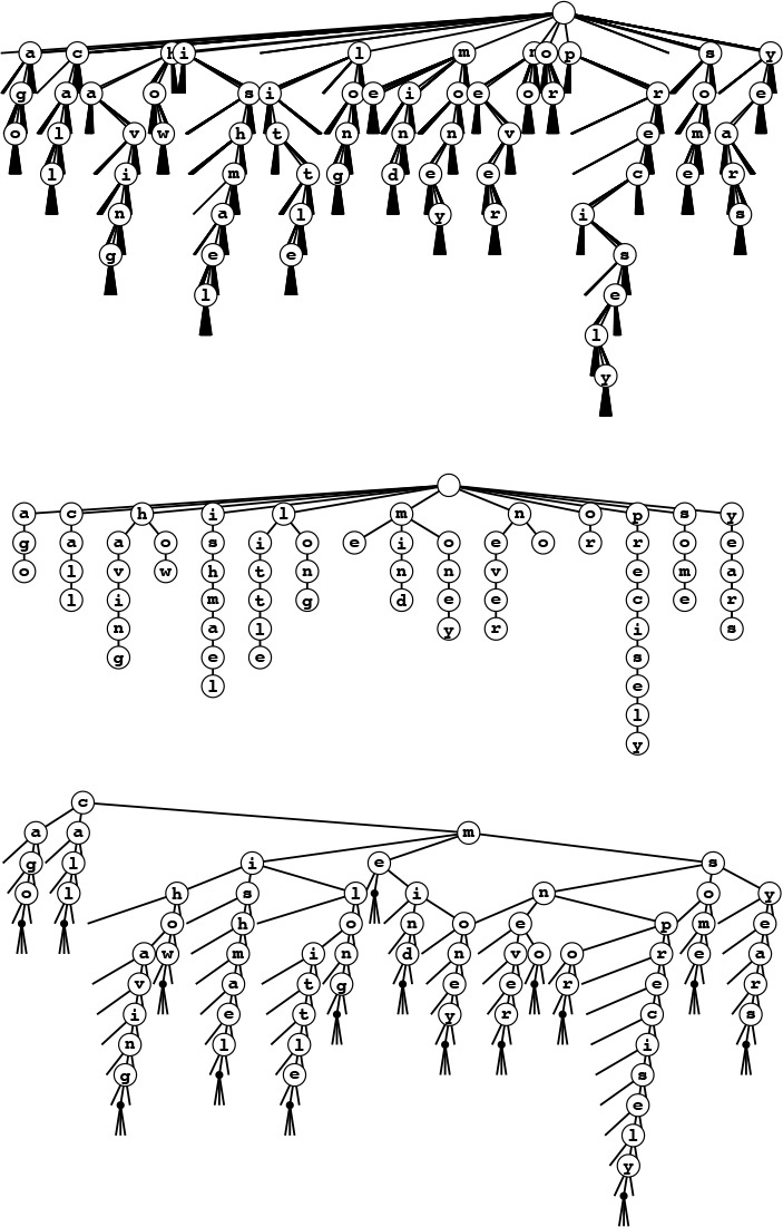
These figures show three different representations of the existence trie for the 16 words call me ishmael some years ago never mind how long precisely having little or no money: The 26-way existence trie (top); the abstract trie with null links removed (center); and the TST representation (bottom). The 26-way trie has too many links, but the TST is an efficient representation of the abstract trie.
The top two tries assume that no key is the prefix of another. For example, adding the key not would result in the key no being lost. We can add a null character to the end of each key to correct this problem, as illustrated in the TST at the bottom.
Figure 15.16 Existence-trie structures
The search algorithm for existence TSTs is so straightforward as nearly to write itself; the insertion algorithm is slightly more complicated, but mirrors directly insertion in existence tries. To search, we compare the first character in the key with the character at the root. If it is less, we take the left link; if it is greater, we take the right link; and if it is equal, we take the middle link and move to the next key character. In each case, we apply the algorithm recursively. We terminate with a search miss if we encounter a null link or if we encounter the end of the search key before encountering NULLdigit in the tree, and we terminate with a search hit if we traverse the middle link in a node whose character is NULLdigit. To insert a new key, we search, then add new nodes for the characters in the tail of the key, just as we did for tries. Program 15.8 gives the details of the implementation of these algorithms, and Figure 15.17 has TSTs that correspond to the tries in Figure 15.15.
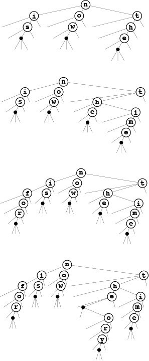
An existence TST has one node for each letter, but only 3 children per node, rather than 26. The top three trees in this figure are the RSTs corresponding to the insertion example in Figure 15.15, with the additional change that an end-of-key character is appended to each key. We can then remove the restriction that no key may be a prefix of another, so, for example, we can insert the key theory (bottom).
Figure 15.17 Existence TSTs
Continuing the correspondence that we have been following between search trees and sorting algorithms, we see that TSTs correspond to three-way radix sorting in the same way that BSTs correspond to quicksort, tries correspond to binary quicksort, and M-way tries correspond to M-way radix sorting. Figure 10.13, which describes the recursive call structure for three-way radix sort, is a TST for that set of keys. The null-links problem for tries corresponds to the empty-bins problem for radix sorting; three-way branching provides an effective solution to both problems.
We can make TSTs more efficient in their use of space by putting keys in leaves at the point where they are distinguished and by eliminating one-way branching between internal nodes as we did for patricia. At the end of this section, we examine an implementation based on the former change.
Property 15.7 A search or insertion in a full TST requires time proportional to the key length. The number of links in a TST is at most three times the number of characters in all the keys.
In the worst case, each key character corresponds to a full R-ary node that is unbalanced, stretched out like a singly linked list. This worst case is extremely unlikely to occur in a random tree. More typically, we might expect to do ln R or fewer byte comparisons at the first level (since the root node behaves like a BST on the R different byte values) and perhaps at a few other levels (if there are keys with a common prefix and up to R different byte values on the character following the prefix), and to do only a few byte comparisons for most characters (since most trie nodes are sparsely populated with non-null links). Search misses are likely to involve only a few byte comparisons, ending at a null link high in the trie, and search hits involve only about one byte comparison per search key character, since most of them are in nodes with one-way branching at the bottom of the trie.
Actual space usage is generally less than the upper bound of three links per character, because keys share nodes at high levels in the tree. We refrain from a precise average-case analysis because TSTs are most useful in practical situations where keys neither are random nor are derived from bizarre worst-case constructions. ![]()
The prime virtue of using TSTs is that they adapt gracefully to irregularities in search keys that are likely to appear in practical applications. There are two main effects. First, keys in practical applications come from large character sets, and usage of particular characters in the character sets is far from uniform—for example, a particular set of strings is likely to use only a small fraction of the possible characters. With TSTs, we can use a 128- or 256-character encoding without having to worry about the excessive costs of nodes with 128- or 256-way branching, and without having to determine which sets of characters are relevant. Character sets for non-Roman alphabets can have thousands of characters—TSTs are especially appropriate for string keys that consist of such characters. Second, keys in practical applications often have a structured format, differing from application to application, perhaps using only letters in one part of the key, only digits in another part of the key, and special characters as delimiters (see Exercise 15.71). For example, Figure 15.18 gives a list of library call numbers from an online library database. For such keys, some of the trie nodes might be represented as unary nodes in the TST (for places where all keys have delimiters); some might be represented as 10-node BSTs (for places where all keys have digits); and still others might be represented as 26-node BSTs (for places where all keys have letters). This structure develops automatically, without any need for special analysis of the keys.
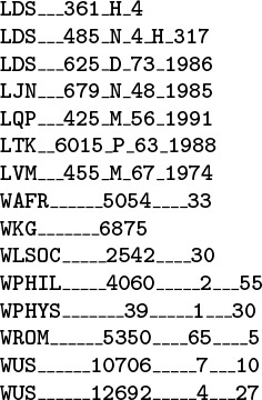
These keys from an online library database illustrate the variability of the structure found in string keys in applications. Some of the characters may appropriately be modeled as random letters, some may be modeled as random digits, and still others have fixed value or structure.
Figure 15.18 Sample string keys (library call numbers)
A second practical advantage of TST-based search over many other algorithms is that search misses are likely to be extremely efficient, even when the keys are long. Often, the algorithm uses just a few byte comparisons (and chases a few pointers) to complete a search miss. As we discussed in Section 15.3, a search miss in a hash table with N keys requires time proportional to the key length (to compute the hash function), and at least lg N key comparisons in a search tree. Even patricia requires lg N bit comparisons for a random search miss.
Table 15.2 gives empirical data in support of the observations in the previous two paragraphs.
These relative timings for construction and search in symbol tables with string keys such as the library call numbers in Figure 15.18 confirm that TSTs, although slightly more expensive to construct, provide the fastest search for search misses with string keys, primarily because the search does not require examination of all the characters in the key.
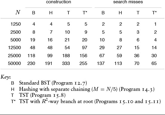
Table 15.2 Empirical study of search with string keys
A third reason that TSTs are attractive is that they support operations more general than the symbol-table operations that we have been considering. For example, Program 15.9 gives a program that allows particular characters in the search key to be unspecified, and prints all keys in the data structure that match the specified digits of the search key. An example is depicted in Figure 15.19. Obviously, with a slight modification, we can adapt this program to visit all the matching keys in the way that we do for sort, rather than just to print them (see Exercise 15.57).
To find all keys in a TST matching the pattern i* (top), we search for i in the BST for the first character. In this example, we find is (the only word that matches the pattern) after two one-way branches. For a less restrictive pattern such as *o* (bottom), we visit all nodes in the BST for the first character, but only those corresponding to o for the second character, eventually finding for and now.
Figure 15.19 TST-based partial-match search
Several other similar tasks are easy to handle with TSTs. For example, we can visit all keys in the data structure that differ from the search key in at most one digit position (see Exercise 15.58). Operations of this type are expensive or impossible with other symbol-table implementations. We shall consider in detail these and many other problems where we do not insist on exact matches in a string search, in Part 5.
Patricia offers several of the same advantages; the main practical advantage of TSTs over patricia tries is that the former access key bytes rather than key bits. One reason that this difference represents an advantage is that machine operations for this purpose are found in many machines, and C provides direct access to bytes in character strings. Another reason is that, in some applications, working with bytes in the data structure naturally reflects the byte orientation of the data itself in some applications—for example, in the partial-match search problem discussed in the previous paragraph (although, as we shall see in Chapter 18, we can speed up partial-match search with judicious use of bit access).
To eliminate one-way branching in TSTs, we note that most of the one-way branching occurs at the tail ends of keys, and does not occur if we evolve to a standard multiway trie implementation, where we keep records in leaves that are placed in the highest level of the trie that distinguishes the keys. We also can maintain a byte index in the same manner as in patricia tries (see Exercise 15.64), but will omit this change, for simplicity. The combination of multiway branching and the TST representation by themselves is quite effective in many applications, but patricia-style collapse of one-way branching will further enhance performance when the keys are such that they are likely to match for long stretches (see Exercise 15.71).
Another easy improvement to TST-based search is to use a large explicit multiway node at the root. The simplest way to proceed is to keep a table of R TSTs: one for each possible value of the first letter in the keys. If R is not large, we might use the first two letters of the keys (and a table of size R2). For this method to be effective, the leading digits of the keys must be well-distributed. The resulting hybrid search algorithm corresponds to the way that a human might search for names in a telephone book. The first step is a multiway decision (“Let’s see, it starts with ‘A’ ”), followed perhaps by some two-way decisions (“It’s before ‘Andrews,’ but after ‘Aitken”’) followed by sequential character matching (“ ‘Algonquin,’ ... No, ‘Algorithms’ isn’t listed, because nothing starts with ‘Algor’!”).
Programs 15.10 and 15.11 are TST-based implementations of the symbol-table search and insert operations that use R-way branching at the root and that keep keys in leaves (so there is no one-way branching once the keys are distinguished). These programs are likely to be among the fastest available for searching with string keys. The underlying TST structure can also support a host of other operations.
In a symbol table that grows to be huge, we may want to adapt the branching factor to the table size. In Chapter 16, we shall see a systematic way to grow a multiway trie so that we can take advantage of multiway radix search for arbitrary file sizes.
Property 15.8 A search or insertion in a TST with items in leaves (no one-way branching at the bottom) and Rt-way branching at the root requires roughly ln N − t ln R byte accesses for N keys that are random bytestrings. The number of links required is Rt (for the root node) plus a small constant times N.
These rough estimates follow immediately from Property 15.6. For the time cost, we assume that all but a constant number of the nodes on the search path (a few at the top) act as random BSTs on R character values, so we simply multiply the time cost by ln R. For the space cost, we assume that the nodes on the first few levels are filled with R character values, and that the nodes on the bottom levels have only a constant number of character values. ![]()
For example, if we have 1 billion random bytestring keys with R = 256, and we use a table of size R2 = 65536 at the top, then a typical search will require about ln 109 − 2 ln 256 ≈ 20.7 − 11.1 = 9.6 byte comparisons. Using the table at the top cuts the search cost by a factor of 2. If we have truly random keys, we can achieve this performance with more direct algorithms that use the leading bytes in the key and an existence table, in the manner discussed in Section 14.6. With TSTs, we can get the same kind of performance when keys have a less random structure.
It is instructive to compare TSTs without multiway branching at the root with standard BSTs, for random keys. Property 15.8 says that TST search will require about ln N byte comparisons, whereas standard BSTs require about ln N key comparisons. At the top of the BST, the key comparisons can be accomplished with just one byte comparison, but at the bottom of the tree multiple byte comparisons may be needed to accomplish a key comparison. This performance difference is not dramatic. The reasons that TSTs are preferable to standard BSTs for string keys are that they provide a fast search miss; they adapt directly to multiway branching at the root; and (most important) they adapt well to bytestring keys that are not random, so no search takes longer than the length of a key in a TST.
Some applications may not benefit from the R-way branching at the root—for example, the keys in the library-call-number example of Figure 15.18 all begin with either L or W. Other applications may call for a higher branching factor at the root—for example, as just noted, if the keys were random integers, we would use as large a table as we could afford. We can use application-specific dependencies of this sort to tune the algorithm to peak performance, but we should not lose sight of the fact that one of the most attractive features of TSTs is that TSTs free us from having to worry about such application-specific dependencies, providing good performance without any tuning.
Perhaps the most important property of tries or TSTs with records in leaves is that their performance characteristics are independent of the key length. Thus, we can use them for arbitrarily long keys. In Section 15.5, we examine a particularly effective application of this kind.
Exercises
![]() 15.48 Draw the existence trie that results when you insert the words
15.48 Draw the existence trie that results when you insert the words now is the time for all good people to come the aid of their party into an initially empty trie. Use 27-way branching.
![]() 15.49 Draw the existence TST that results when you insert the words
15.49 Draw the existence TST that results when you insert the words now is the time for all good people to come the aid of their party into an initially empty TST.
![]() 15.50 Draw the 4-way trie that results when you insert items with the keys
15.50 Draw the 4-way trie that results when you insert items with the keys 01010011 00000111 00100001 01010001 11101100 00100001 10010101 0100-1010 into an initially empty trie, using 2-bit bytes.
![]() 15.51 Draw the TST that results when you insert items with the keys
15.51 Draw the TST that results when you insert items with the keys 0101-0011 00000111 00100001 01010001 11101100 00100001 10010101 01001010 into an initially empty TST, using 2-bit bytes.
![]() 15.52 Draw the TST that results when you insert items with the keys
15.52 Draw the TST that results when you insert items with the keys 0101-0011 00000111 00100001 01010001 11101100 00100001 10010101 01001010 into an initially empty TST, using 4-bit bytes.
![]() 15.53 Draw the TST that results when you insert items with the library-call-number keys in Figure 15.18 into an initially empty TST.
15.53 Draw the TST that results when you insert items with the library-call-number keys in Figure 15.18 into an initially empty TST.
![]() 15.54 Modify our multiway-trie search and insertion implementation (Program 15.7) to work under the assumption that keys are (fixed-length) w-byte words (so no end-of-key indication is necessary).
15.54 Modify our multiway-trie search and insertion implementation (Program 15.7) to work under the assumption that keys are (fixed-length) w-byte words (so no end-of-key indication is necessary).
![]() 15.55 Modify our TST search and insertion implementation (Program 15.8) to work under the assumption that keys are (fixed-length) w-byte words (so no end-of-key indication is necessary).
15.55 Modify our TST search and insertion implementation (Program 15.8) to work under the assumption that keys are (fixed-length) w-byte words (so no end-of-key indication is necessary).
15.56 Run empirical studies to compare the time and space requirements of an 8-way trie built with random integers using 3-bit bytes, a 4-way trie built with random integers using 2-bit bytes, and a binary trie built from the same keys, for N = 103, 104, 105, and 106 (see Exercise 15.14).
15.57 Modify Program 15.9 such that it visits, in the same manner as sort, all the nodes that match the search key.
![]() 15.58 Write a function that prints all the keys in a TST that differ from the search key in at most
15.58 Write a function that prints all the keys in a TST that differ from the search key in at most k positions, for a given integer k.
![]() 15.59 Give a full characterization of the worst-case internal path length of an R-way trie with N distinct w-bit keys.
15.59 Give a full characterization of the worst-case internal path length of an R-way trie with N distinct w-bit keys.
![]() 15.60 Implement the sort, delete, select, and join operations for a multiwaytrie–based symbol table.
15.60 Implement the sort, delete, select, and join operations for a multiwaytrie–based symbol table.
![]() 15.61 Implement the sort, delete, select, and join operations for a TST-based symbol table.
15.61 Implement the sort, delete, select, and join operations for a TST-based symbol table.
![]() 15.62 Write a program that prints out all keys in an R-way trie that have the same initial
15.62 Write a program that prints out all keys in an R-way trie that have the same initial t bytes as a given search key.
![]() 15.63 Modify our multiway-trie search and insertion implementation (Program 15.7) to eliminate one-way branching in the way that we did for patricia tries.
15.63 Modify our multiway-trie search and insertion implementation (Program 15.7) to eliminate one-way branching in the way that we did for patricia tries.
![]() 15.64 Modify our TST search and insertion implementation (Program 15.8) to eliminate one-way branching in the way that we did for patricia tries.
15.64 Modify our TST search and insertion implementation (Program 15.8) to eliminate one-way branching in the way that we did for patricia tries.
15.65 Write a program to balance the BSTs that represent the internal nodes of a TST (rearrange them such that all their external nodes are on one of two levels).
15.66 Write a version of insert for TSTs that maintains a balanced-tree representation of all the internal nodes (see Exercise 15.65).
![]() 15.67 Give a full characterization of the worst-case internal path length of a TST with N distinct w-bit keys.
15.67 Give a full characterization of the worst-case internal path length of a TST with N distinct w-bit keys.
15.68 Write a program that generates random 80-byte string keys (see Exercise 10.19). Use this key generator to build a 256-way trie with N random keys, for N = 103, 104, 105, and 106, using search, then insert on search miss. Instrument your program to print out the total number of nodes in each trie and the total amount of time taken to build each trie.
15.69 Answer Exercise 15.68 for TSTs. Compare your performance results with those for tries.
15.70 Write a key generator that generates keys by shuffling a random 80-byte sequence (see Exercise 10.21). Use this key generator to build a 256-way trie with N random keys, for N = 103, 104, 105, and 106, using search, then insert on search miss. Compare your performance results with those for the random case (see Exercise 15.68).
![]() 15.71 Write a key generator that generates 30-byte random strings made up of three fields: a 4-byte field with one of a set of 10 given strings; a 10-byte field with one of a set of 50 given strings; a 1-byte field with one of two given values; and a 15-byte field with random left-justified strings of letters equally likely to be four through 15 characters long (see Exercise 10.23). Use this key generator to build a 256-way trie with N random keys, for N = 103, 104, 105, and 106, using search, then insert on search miss. Instrument your program to print out the total number of nodes in each trie and the total amount of time taken to build each trie. Compare your performance results with those for the random case (see Exercise 15.68).
15.71 Write a key generator that generates 30-byte random strings made up of three fields: a 4-byte field with one of a set of 10 given strings; a 10-byte field with one of a set of 50 given strings; a 1-byte field with one of two given values; and a 15-byte field with random left-justified strings of letters equally likely to be four through 15 characters long (see Exercise 10.23). Use this key generator to build a 256-way trie with N random keys, for N = 103, 104, 105, and 106, using search, then insert on search miss. Instrument your program to print out the total number of nodes in each trie and the total amount of time taken to build each trie. Compare your performance results with those for the random case (see Exercise 15.68).
15.72 Answer Exercise 15.71 for TSTs. Compare your performance results with those for tries.
15.73 Develop an implementation of search and insert for bytestring keys using multiway digital search trees.
![]() 15.74 Draw the 27-way DST (see Exercise 15.73) that results when you insert items with the keys
15.74 Draw the 27-way DST (see Exercise 15.73) that results when you insert items with the keys now is the time for all good people to come the aid of their party into an initially empty DST.
![]() 15.75 Develop an implementation of multiway-trie search and insertion using linked lists to represent the trie nodes (as opposed to the BST representation that we use for TSTs). Run empirical studies to determine whether it is more efficient to use ordered or unordered lists, and to compare your implementation with a TST-based implementation.
15.75 Develop an implementation of multiway-trie search and insertion using linked lists to represent the trie nodes (as opposed to the BST representation that we use for TSTs). Run empirical studies to determine whether it is more efficient to use ordered or unordered lists, and to compare your implementation with a TST-based implementation.
15.5 Text-String–Index Algorithms
In Section 12.7, we considered the process of building a string index, and we used a binary search tree with string pointers to provide the capability to determine whether or not a given key string appears in a huge text. In this section, we look at more sophisticated algorithms using multiway tries, but starting from the same point of departure. We consider each position in the text to be the beginning of a string key that runs all the way to the end of the text and build a symbol table with these keys, using string pointers. The keys are all different (for example, they are of different lengths), and most of them are extremely long. The purpose of a search is to determine whether or not a given search key is a prefix of one of the keys in the index, which is equivalent to discovering whether the search key appears somewhere in the text string.
A search tree that is built from keys defined by string pointers into a text string is called a suffix tree. We could use any algorithm that can admit variable-length keys. Trie-based methods are particularly suitable, because (except for the trie methods that do one-way branching at the tails of keys) their running time does not depend on the key length, but rather depends on only the number of digits required to distinguish among the keys. This characteristic lies in direct contrast to, for example, hashing algorithms, which do not apply immediately to this problem because their running time is proportional to the key length.
Figure 15.20 gives examples of string indexes built with BSTs, patricia, and TSTs (with leaves). These indexes use just the keys starting at word boundaries; an index starting at character boundaries would provide a more complete index, but would use significantly more space.
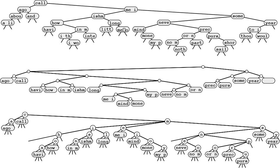
These diagrams show text-string indexes built from the text call me ishmael some years ago never mind how long precisely ... using a BST (top), a patricia trie (center), and a TST (bottom). Nodes with string pointers are depicted with the first four characters at the point referenced by the pointer.
Figure 15.20 Text-string index examples
Strictly speaking, even a random string text does not give rise to a random set of keys in the corresponding index (because the keys are not independent). However, we rarely work with random texts in practical indexing applications, and this analytic discrepancy will not stop us from taking advantage of the fast indexing implementations that are possible with radix methods. We refrain from discussing the detailed performance characteristics when we use each of the algorithms to build a string index, because many of the same tradeoffs that we have discussed for general symbol tables with string keys also hold for the string-index problem.
For a typical text, standard BSTs would be the first implementation that we might choose, because they are simple to implement (see Program 12.10). For typical applications, this solution is likely to provide good performance. One byproduct of the interdependence of the keys—particularly when we are building a string index for each character position—is that the worst case for BSTs is not a particular concern for huge texts, since unbalanced BSTs occur with only bizarre constructions.
Patricia was originally designed for the string-index application. To use Programs 15.5 and 15.4, we need only to provide an implementation of bit that, given a string pointer and an integer i, returns the ith bit of the string (see Exercise 15.81). In practice, the height of a patricia trie that implements a text string index will be logarithmic. Moreover, a patricia trie will provide fast search implementations for misses because we do not need to examine all the bytes of the key.
TSTs afford several of the performance advantages of patricia, are simple to implement, and take advantage of built-in byte-access operations that are typically found on modern machines. They also are amenable to simple implementations, such as Program 15.9, that can solve search problems more complicated than fully matching a search key. To use TSTs to build a string index, we need to remove the code that handles ends of keys in the data structure, since we are guaranteed that no string is a prefix of another, and thus we never will be comparing strings to their ends. This modification includes changing the definition of eq in the item-type interface to regard two strings as equal if one is a prefix of the other, as we did in Section 12.7, since we will be comparing a (short) search key against a (long) text string, starting at some position in the text string. A third change that is convenient is to keep string pointers in each node, rather than characters, so that every node in the tree refers to a position in the text string (the position in the text string following the first occurrence of the character string defined by the characters on equal branches from the root to that node). Implementing these changes is an interesting and informative exercise that leads to a flexible and efficient text-string–index implementation (see Exercise 15.80).
Despite all the advantages that we have been discussing, there is an important fact that we are overlooking when considering the use of BSTs, patricia tries, or TSTs for typical text indexing applications: the text itself is usually fixed, so we do not need to support the dynamic insert operations that we have become accustomed to supporting. That is, we typically build the index once, then use it for a huge number of searches, without ever changing it. Therefore, we may not need dynamic data structures like BSTs, patricia tries or TSTs at all. The basic algorithm that is appropriate for handling this situation is binary search, with string pointers (see Section 12.4). The index is a set of string pointers; index construction is a string pointer sort. The primary advantage of using binary search over a dynamic data structure is the space savings. To index a text string at N positions using binary search, we need just N string pointers; in contrast, to index a string at N positions using a tree-based method, we need at least 3N pointers (one string pointer, to the text, and two links). Text indexes are typically huge, so binary search might be preferred because it provides guaranteed logarithmic search time but uses one-third the amount of memory used by tree-based methods. If sufficient memory space is available, however, TSTs will lead to a faster search for many applications because it moves through the key without retracing its steps, and binary search does not do so.
If we have a huge text but plan to perform only a small number of searches, then building a full index is not likely to be justified. In Part 5, we consider the string-search problem, where we want to determine quickly whether a given text contains a given search key, without any preprocessing. We shall also consider a number of string-search problems that are between the two extremes of doing no preprocessing and building a full index for a huge text.
Exercises
![]() 15.76 Draw the 26-way DST that results when you build a text-string index from the words
15.76 Draw the 26-way DST that results when you build a text-string index from the words now is the time for all good people to come the aid of their party.
![]() 15.77 Draw the 26-way trie that results when you build a text-string index from the words
15.77 Draw the 26-way trie that results when you build a text-string index from the words now is the time for all good people to come the aid of their party.
![]() 15.78 Draw the TST that results when you build a text-string index from the words
15.78 Draw the TST that results when you build a text-string index from the words now is the time for all good people to come the aid of their party, in the style of Figure 15.20.
![]() 15.79 Draw the TST that results when you build a text-string index from the words
15.79 Draw the TST that results when you build a text-string index from the words now is the time for all good people to come the aid of their party, using the implementation described in the text, where the TST contains string pointers at every node.
![]() 15.80 Modify the TST search and insertion implementations in Programs 15.10 and 15.11 to provide a TST-based string index.
15.80 Modify the TST search and insertion implementations in Programs 15.10 and 15.11 to provide a TST-based string index.
![]() 15.81 Implement an interface that allows patricia to process C string keys (that is, arrays of characters) as though they were bitstrings.
15.81 Implement an interface that allows patricia to process C string keys (that is, arrays of characters) as though they were bitstrings.
![]() 15.82 Draw the patricia trie that results when you build a text string index from the words
15.82 Draw the patricia trie that results when you build a text string index from the words now is the time for all good people to come the aid of their party, using a 5-bit binary coding with the ith letter in the alphabet represented by the binary representation of i.
15.83 Explain why the idea of improving binary search using the same basic principle on which TSTs are based (comparing characters rather than strings) is not effective.
15.84 Find a large (at least 106 bytes) text file on your system, and compare the height and internal path length of a standard BST, patricia trie, and TST, when you use these methods to build an index from that file.
15.85 Run empirical studies to compare the height and internal path length of a standard BST, patricia trie, and TST, when you use these methods to build an index from a text string consisting of N random characters from a 32-character alphabet, for N = 103, 104, 105, and 106.
![]() 15.86 Write an efficient program to determine the longest repeated sequence in a huge text string.
15.86 Write an efficient program to determine the longest repeated sequence in a huge text string.
![]() 15.87 Write an efficient program to determine the 10-character sequence that occurs most frequently in a huge text string.
15.87 Write an efficient program to determine the 10-character sequence that occurs most frequently in a huge text string.
![]() 15.88 Build a string index that supports an operation that returns the number of occurrences of its argument in the indexed text, and supports, in the same manner as sort, a search operation that visits all the text positions that match the search key.
15.88 Build a string index that supports an operation that returns the number of occurrences of its argument in the indexed text, and supports, in the same manner as sort, a search operation that visits all the text positions that match the search key.
![]() 15.89 Describe a text string of N characters for which a TST-based string index will perform particularly badly. Estimate the cost of building an index for the same string with a BST.
15.89 Describe a text string of N characters for which a TST-based string index will perform particularly badly. Estimate the cost of building an index for the same string with a BST.
15.90 Suppose that we want to build an index for a random N-bit string, for bit positions that are a multiple of 16. Run empirical studies to determine which of the bytesizes 1, 2, 4, 8, or 16 leads to the lowest running times to construct a TST-based index, for N = 103, 104, 105, and 106.