Chapter 8. Printing in Excel
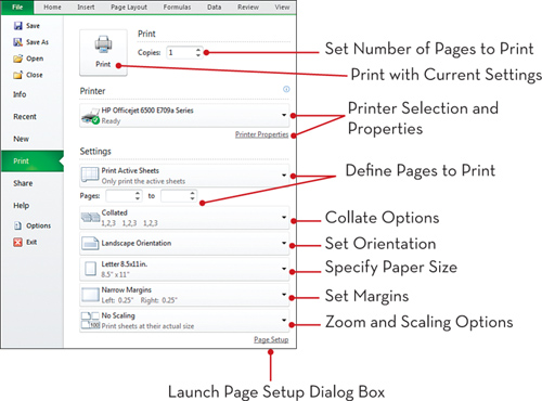
Printing options in Excel 2010 haven’t changed that much since Excel 2003. However, it would be foolish not to mention that Excel 2010 does consolidate most printing options into the Backstage View. You can get to the Backstage View by clicking on the File tab on the Ribbon. Although there are several methods of getting to print options, the Excel 2010’s Backstage View provides an easy way to quickly configure Excel’s print options.
And as you will see, Excel does have a plethora of print options. Don’t worry—Excel does allow you to print your worksheets by using basic print settings if that’s all you need. But Excel also offers a bevy of settings that enable you to enhance your printouts. Some of these options include orientation adjustments, scaling, paper size options, page numbering, adding headers, adding footers, and more.
In this chapter, you get a tour of the printing options available to you.
Print Options Via the Backstage View
Using Print Preview
Worksheets with lots of data can generate large print jobs, possibly containing hundreds of pages. Waiting until all these pages are printed to verify that the information is printed correctly can cost a lot in both time and printing supplies. To help prevent printing mistakes, use Print Preview to ensure that all the necessary elements appear on the pages before printing.
![]()
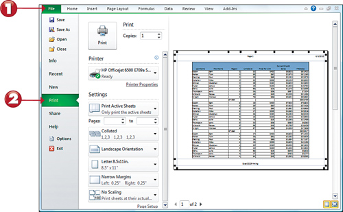
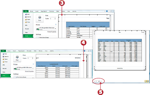
![]() With the worksheet you want to print open, click the File tab on the ribbon.
With the worksheet you want to print open, click the File tab on the ribbon.
![]() Click Print to display the worksheet’s Print Preview.
Click Print to display the worksheet’s Print Preview.
Note: Paging Through the Print Preview
![]()
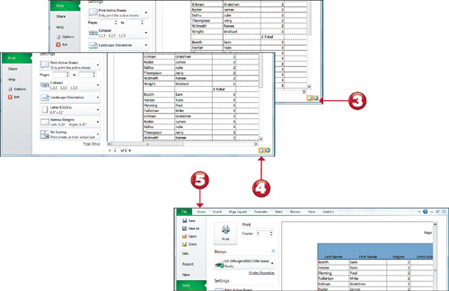
Note the navigation spinner in the lower left-hand corner of the Print Preview. In this case, the navigation spinner reads 1 of 2. You not only can use this to determine how many pages will be printed, but you can cycle through the pages by clicking the left and right arrows.
Tip: Page Break Preview Button
![]()
Click Page Break Preview on the View Tab to see and modify exactly what is selected to print (in the print area). If you haven’t set the print area, see “Setting the Print Area.”
![]() Click the Zoom button to increase the viewable size of the worksheet in Print Preview mode. (Click Zoom again to return to the original page size.)
Click the Zoom button to increase the viewable size of the worksheet in Print Preview mode. (Click Zoom again to return to the original page size.)
![]() Click Margins to toggle between displaying the margin indicators, which you can drag to set more or less of your worksheet to print.
Click Margins to toggle between displaying the margin indicators, which you can drag to set more or less of your worksheet to print.
![]() Click the Home tab to return to the worksheet’s Normal view.
Click the Home tab to return to the worksheet’s Normal view.
![]()
Tip: Zoom with your Mouse Wheel
![]()
You can also use your mouse wheel to zoom in and out of a print preview. Hold down the Ctrl key on your keyboard while you spin your mouse wheel. This increases or reduces magnification of your Print Preview depending on the direction you spin (up or down).

Setting the Print Area
Worksheets can include several rows and columns; setting the print area enables you to specify which rows and columns to print. If you don’t set a print area, all cells that contain data will print. The worksheet in this task contains four tables that span seven pages. By default, all will print unless you set a print area.
![]()
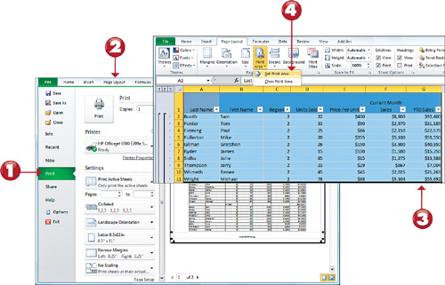
![]() Click the File tab, then select Print to see a Print Preview of your worksheet.
Click the File tab, then select Print to see a Print Preview of your worksheet.
![]() Should your print area need adjusting, click on the Page Layout menu option to return to Normal view.
Should your print area need adjusting, click on the Page Layout menu option to return to Normal view.
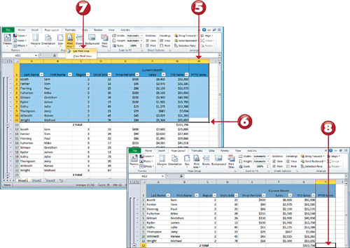
![]() Select the exact cells you want to print (in this example, all the cells in the first two tables in this worksheet).
Select the exact cells you want to print (in this example, all the cells in the first two tables in this worksheet).
![]() Click the Print Area command on the ribbon, and select Set Print Area. This will store the print area as part of the worksheet. Now, only the cells in the print area will print.
Click the Print Area command on the ribbon, and select Set Print Area. This will store the print area as part of the worksheet. Now, only the cells in the print area will print.
![]()
Tip: Another Way to Choose the Print Area
![]()
You can also Set the Print Area from the traditional Page Setup dialog box. To get there, go to the Page Layout tab and click the Page Setup dialog launcher. Once the Page Setup dialog box activates, you can click on the Sheet tab. There, you can set the Print Area input to the cell range you want to print.
![]() Insert a row or column into your worksheet (PYTD Sales, for example). Parts of the table now fall outside the current print area.
Insert a row or column into your worksheet (PYTD Sales, for example). Parts of the table now fall outside the current print area.
![]() Select the exact cells you want to print (now including the extra column).
Select the exact cells you want to print (now including the extra column).
![]() To reset the print area to include the new row or column, choose Print Area from the Page Layout Tab, and select Set Print Area.
To reset the print area to include the new row or column, choose Print Area from the Page Layout Tab, and select Set Print Area.
![]() Your new print area is stored as part of this worksheet. If the new print area falls outside the margins, see the next task.
Your new print area is stored as part of this worksheet. If the new print area falls outside the margins, see the next task.
![]()
Note: Long and Short Dashes
![]()
The long dashed lines in your worksheet indicate the print area, and the smaller dashed lines indicate the current page margins. If your print area data falls outside the current page margins, you need to alter the page margins.
Adjusting Page Margins
Margins affect where data is printed on a page. They also determine where headers and footers are printed. Occasionally, margins might need to be changed to make room for a letterhead or logo on preprinted stationery. When in Print Preview mode, Excel enables you to simultaneously alter your column widths and margins.
![]()
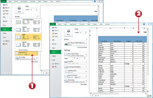
![]() When in Print Preview mode, if you have a page that displays some carryover data from another page, click the Margins button. You can select from one of the default margin settings or customize.
When in Print Preview mode, if you have a page that displays some carryover data from another page, click the Margins button. You can select from one of the default margin settings or customize.
![]() Excel activates Print Preview’s margin lines. Press page up or page down to display the page in your worksheet on which you want to fit all the data.
Excel activates Print Preview’s margin lines. Press page up or page down to display the page in your worksheet on which you want to fit all the data.
Note: Entering Specific Margins
![]()
If you need to enter specific margin measurements, the Page Setup dialog box is a better option. Go to the Page Layout tab and click the Page Setup dialog launcher. Once the Page Setup dialog box activates, you can click on the Margins tab and alter the margins as necessary (Left, Right, Top, Bottom, Header, Footer). Click the OK button to return to your worksheet or Print to print immediately.

![]() Drag the Left Margin line from the default 1” to 0.34”. (You can see the exact measurement in the bottom-left corner of the screen.)
Drag the Left Margin line from the default 1” to 0.34”. (You can see the exact measurement in the bottom-left corner of the screen.)
![]() Click and drag the Right Margin line from the default 1” to 0.34”. (Again, you can see the exact measurement in the bottom-left corner of the screen.)
Click and drag the Right Margin line from the default 1” to 0.34”. (Again, you can see the exact measurement in the bottom-left corner of the screen.)
![]() Thanks to the margin change, the total number of pages to print is reduced.
Thanks to the margin change, the total number of pages to print is reduced.
![]()

Inserting Page Breaks
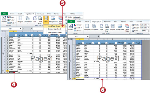
When a worksheet page is filled to the margins with data, Excel automatically inserts a page break for you. There may be times, however, when you want to manually insert a page break. For example, if you create a report with multiple topic sections, you might want each topic to begin on a new page. Inserting a page break enables you to print each page separately. The best way to insert page breaks is using Page Break Preview view (instead of Normal view).
![]()
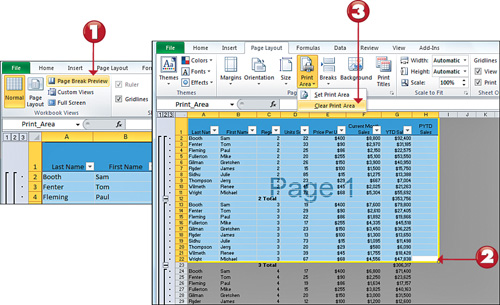
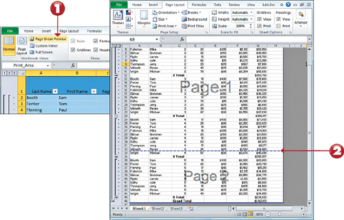
![]() Open the View tab and choose Page Break Preview to change to Page Break Preview mode.
Open the View tab and choose Page Break Preview to change to Page Break Preview mode.
![]() Press the page up and page down keys on the keyboard to move through your worksheet in Page Break Preview. Notice that cells outside the print area are grayed out.
Press the page up and page down keys on the keyboard to move through your worksheet in Page Break Preview. Notice that cells outside the print area are grayed out.
![]() Open the Page Layout tab, choose Print Area, and select Clear Print Area to eliminate any current print area settings.
Open the Page Layout tab, choose Print Area, and select Clear Print Area to eliminate any current print area settings.
Note: Removing Page Breaks
![]()
To remove a page break, place the active cell so that one of the cell borders is touching the page break line. Then, select the Page Layout tab and choose Remove Page Break. (You can also do this in Normal view.)
Note: Page Break Intersection
![]()
A page break is always inserted as an intersection between rows and columns. If the active cell isn’t in the first column, the page break will be inserted as four quadrants.
![]() Click the cell below and in the left-most column in which you want to insert a page break.
Click the cell below and in the left-most column in which you want to insert a page break.
![]() On the Page Layout tab choose Breaks, Insert Page Break to insert the page break.
On the Page Layout tab choose Breaks, Insert Page Break to insert the page break.
![]() The page break is inserted.
The page break is inserted.
![]()
Tip: Why Not Simply Add More Rows
![]()
Suppose you want each of two tables that fit on one page to print on separate pages. Instead of inserting a page break, you could add several blank rows to the end of the first table, which automatically kicks the second one onto a second page. If, however, you later add any rows to the first table and forget to delete the same number of blank rows before the second one, the tables might not print correctly.
![]()
Working in Page Break Preview Mode
Page Break Preview mode displays the area you have selected for your set print area. It also enables you to click and drag where your page breaks are instead of using the Insert, Page Break command. You can also edit the text and data just as you can in Normal view.
![]()
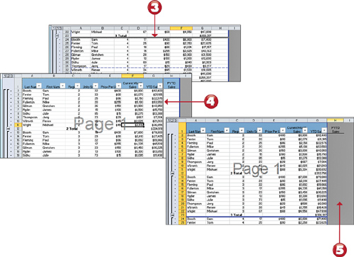
![]() Click Page Break Preview from the View tab on the ribbon. If a print area has been set, it is displayed; if not, the entire worksheet is displayed.
Click Page Break Preview from the View tab on the ribbon. If a print area has been set, it is displayed; if not, the entire worksheet is displayed.
![]() Move through the worksheet to find page breaks (if any). Naturally occurring page breaks appear as blue dashed lines, and inserted page breaks appear as solid blue lines.
Move through the worksheet to find page breaks (if any). Naturally occurring page breaks appear as blue dashed lines, and inserted page breaks appear as solid blue lines.
Note: Clearing the Print Area
![]()
If you need to set only the print area to print a portion of data in your worksheet once, you probably want to clear the print area after you print. Go to the Page Layout tab, click the Print Area command, and select Clear Print Area.
![]() To move a page break that is poorly placed, click and drag it to a better location. (Moving a natural page break changes it to an inserted break—solid-blue.)
To move a page break that is poorly placed, click and drag it to a better location. (Moving a natural page break changes it to an inserted break—solid-blue.)
![]() To exclude a column or data to the right of your set print area, click and drag the vertical page break.
To exclude a column or data to the right of your set print area, click and drag the vertical page break.
![]() The excluded column outside the print area is grayed out.
The excluded column outside the print area is grayed out.
![]()
Tip: Removing a Page Break
![]()
To remove a page break in Page Break Preview mode, click and drag the page break line off to the right/left/top/bottom of the worksheet.

Printing a Worksheet on One Page
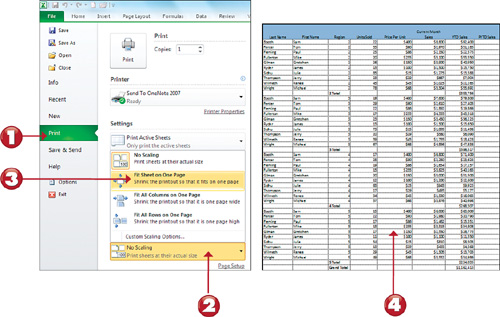
By default, Excel prints your worksheet at a scale of 100%. You can decrease this percentage if you want to fit more data on a page, or increase it to fit less data on a page. In addition, you can have Excel fit your entire worksheet on one page. (If your worksheet is large, the data might become too tiny to read when scaled down.)
![]()
![]() Go the File tab and click Print.
Go the File tab and click Print.
![]() Click the Zoom and Scaling drop-down.
Click the Zoom and Scaling drop-down.
![]() Select the Fit Sheet on One Page option.
Select the Fit Sheet on One Page option.
![]() Your worksheet appears in Print Preview mode, all on one page.
Your worksheet appears in Print Preview mode, all on one page.
![]()
Tip: Changing from Letter to Legal
![]()
To choose a different paper size for your printout, click the Paper Size dropdown on the Print pane of the Backstage View. There, you can select Legal. The scaling setting automatically adjusts to the selected paper size.
Note: Returning to the Default Scale
![]()
When you want to return the preview of your worksheet to the default scale, return the Scaling dropdown to the No Scaling option.
Printing in Portrait or Landscape Orientation
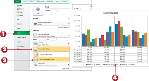
Not all Excel reports are the same. Some reports have just a few columns, while others are very wide with many columns. Depending on your report, you will either print in Portrait or Landscape orientation. The default orientation in Excel is Portrait, meaning the report can fit vertically on one page without the sides being cut off. Landscape orientation means that your page is printed horizontally (on its side) so that you get that extra room on the sides for more columns to fit.
![]()
![]() Go the File tab and click Print.
Go the File tab and click Print.
![]() Click the Orientation drop-down.
Click the Orientation drop-down.
![]() Select the Landscape Orientation option.
Select the Landscape Orientation option.
![]() Your report is now in Landscape orientation.
Your report is now in Landscape orientation.
![]()

Centering a Worksheet on a Page
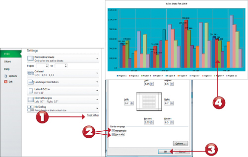
If you want a cleaner, more professional looking printout for a presentation, you might want to center your worksheet data on the page before you print it. This is a particularly good idea if you plan to print your worksheet on one page.
![]()
![]() Go to the Print pane in the Backstage View and click the Page Setup link.
Go to the Print pane in the Backstage View and click the Page Setup link.
![]() On the Margins tab, click the Horizontally and/or Vertically check boxes in the Center on page area.
On the Margins tab, click the Horizontally and/or Vertically check boxes in the Center on page area.
![]() Click OK.
Click OK.
![]() Your worksheet appears in Print Preview mode, centered.
Your worksheet appears in Print Preview mode, centered.
![]()
Tip: Centering Vertically or Horizontally
![]()
You don’t have to center your data both vertically and horizontally. You can choose one or the other, depending on how you want your printed worksheet to look.
Printing Gridlines and Row/Column Headers
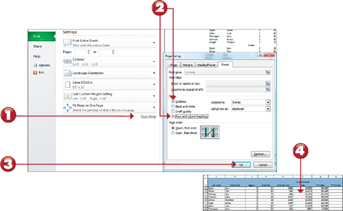
By default, Excel doesn’t print worksheet gridlines or row/column headers. You can, however, instruct Excel to print them. Gridlines help you read information in a printed worksheet, keeping rows and columns of data visually organized. Row and column headers can help you quickly find data in your worksheet.
![]()
![]() Go to the Print pane in the Backstage View and click the Page Setup link.
Go to the Print pane in the Backstage View and click the Page Setup link.
![]() On the Sheet tab, click the Gridlines and Row and column headings check boxes in the Print area to select them.
On the Sheet tab, click the Gridlines and Row and column headings check boxes in the Print area to select them.
![]() Click OK.
Click OK.
![]() Your worksheet appears in Print Preview mode with gridlines and row/column headers visible.
Your worksheet appears in Print Preview mode with gridlines and row/column headers visible.
![]()
Note: Repeating Titles
![]()
Displaying row and column headers is not the same as printing repeating titles. Repeating titles are column headers and row headers that you have assigned in your worksheet. For more information, see the task “Printing Repeating Row and Column Titles” later in this chapter.
Printing Cell Comments
Some cells contain data or formulas that require an explanation or special attention. Comments provide a way to attach this type of information to individual cells. A red triangle in the upper-right corner of the cell indicates that a comment is present. Check Chapter 3, “Entering and Managing Data,” for more information on using comments.
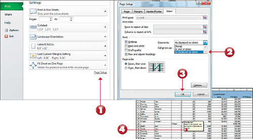
This task shows you how to print your worksheets so that the printouts include the information in your comments, either as they appear in the worksheet or at the end of the worksheet.
![]()
![]() Go to the Print pane in the Backstage View and click the Page Setup link.
Go to the Print pane in the Backstage View and click the Page Setup link.
![]() On the Sheet tab, click the Comments field down arrow and choose either At End of Sheet, to print the comments, As Displayed on Sheet, or (None).
On the Sheet tab, click the Comments field down arrow and choose either At End of Sheet, to print the comments, As Displayed on Sheet, or (None).
![]() Click OK.
Click OK.
![]() View your worksheet in Print Preview mode to review the comments as displayed in your worksheet (as in this example) or at the end of your worksheet.
View your worksheet in Print Preview mode to review the comments as displayed in your worksheet (as in this example) or at the end of your worksheet.
![]()
Note: As Displayed on Sheet
![]()
You must have your comments “showing” in your worksheet (choose View, Comments) for them to display when the As Displayed on Sheet Option is selected. If they aren’t showing, they won’t display in the printout or in Print Preview.
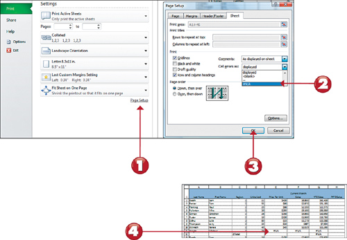
Printing Cell Error Indicators
When you print worksheets for friends or colleagues (or even yourself), calculation errors that appear on your worksheet can create a negative impression, which is why they’re not printed by default. If you want these errors to be visible in your printout, however, you can display them or replace them with any of the following: <blank>, --, or #N/A.
![]()
![]() Go to the Print pane in the Backstage View and click the Page Setup link.
Go to the Print pane in the Backstage View and click the Page Setup link.
![]() On the Sheet tab, click the down arrow next to the Cell errors as field and choose displayed, <blank>, --, or #N/A depending on how you want errors to be displayed.
On the Sheet tab, click the down arrow next to the Cell errors as field and choose displayed, <blank>, --, or #N/A depending on how you want errors to be displayed.
![]() Click OK.
Click OK.
![]() View your worksheet in Print Preview mode to review how cells containing errors display.
View your worksheet in Print Preview mode to review how cells containing errors display.
![]()
Note: Errors That Print
![]()
All the error messages explained in Chapter 5, “Working with Formulas and Functions,” (#DIV/o!, #Name?, #Value!, #REF!, and Circular Reference errors) will print.
Printing Repeating Row and Column Titles
You might have noticed that when a worksheet spans multiple pages, it is difficult to keep the column and row titles organized. A quick way to rectify this is to make particular titles repeat on each page of the printed worksheet.
![]()
![]() Go to the Page Layout tab and click the Page Setup dialog launcher.
Go to the Page Layout tab and click the Page Setup dialog launcher.
![]() Click the Rows to repeat at top selection box in the Print titles area. Excel shrinks the Page Setup dialog box, making your focus the worksheet on your desktop.
Click the Rows to repeat at top selection box in the Print titles area. Excel shrinks the Page Setup dialog box, making your focus the worksheet on your desktop.
![]() Click the row containing the titles that you want to repeat on each page of your worksheet, and press Enter to reopen the Page Setup dialog box with your selection inserted.
Click the row containing the titles that you want to repeat on each page of your worksheet, and press Enter to reopen the Page Setup dialog box with your selection inserted.
![]() Click OK. If you want, view the worksheet in Print Preview mode to get an idea of what your printed worksheet will look like with repeating row headings.
Click OK. If you want, view the worksheet in Print Preview mode to get an idea of what your printed worksheet will look like with repeating row headings.
![]()
Note: Repeating Column Headings
![]()
To repeat column headings across several pages, follow the steps in this task, but click the Columns to repeat at the left selection box in step 2. Then, click the columns you want to repeat, and proceed as normal.
Adding Headers and Footers
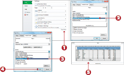
Headers and footers appear at the top and bottom of printed pages of Excel worksheets and can display the filename, the date and time the worksheet was printed, and the worksheet’s name, or you can create your own custom header or footer.
![]()
![]() Go to the Print pane in the Backstage View and click the Page Setup link.
Go to the Print pane in the Backstage View and click the Page Setup link.
![]() On the Header/Footer tab, click the down arrow next to the Header field, and scroll through the header options. If you see one you like, click it to see what it looks like.
On the Header/Footer tab, click the down arrow next to the Header field, and scroll through the header options. If you see one you like, click it to see what it looks like.
![]() Click the down arrow next to the Footer, and scroll through the footer options. If you see one you like, click it to see what it looks like.
Click the down arrow next to the Footer, and scroll through the footer options. If you see one you like, click it to see what it looks like.
![]() Click OK.
Click OK.
![]() You can view the worksheet in Print Preview mode to get an idea of what your printed worksheet will look like with headers and footers.
You can view the worksheet in Print Preview mode to get an idea of what your printed worksheet will look like with headers and footers.
![]()
Printing Worksheets
Printing a worksheet, workbook, or chart sheet is quite simple, but setting the options for printing can be complex. The number of options that must be set before printing depends on the amount of data stored in the workbook, how it is arranged, how much of it needs to be printed, and how you want the printout to look.
![]()
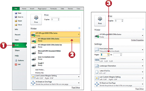
![]() Go the File tab and click Print.
Go the File tab and click Print.
![]() Click the down arrow next to the Printer Name field to choose the printer or fax you want to use.
Click the down arrow next to the Printer Name field to choose the printer or fax you want to use.
![]() In the Print range area, click Page(s) From and To, and type the pages you want to include in the range (for example, from 2 to 5) or keep the All (default).
In the Print range area, click Page(s) From and To, and type the pages you want to include in the range (for example, from 2 to 5) or keep the All (default).
Note: Vertical or Horizontal Page Order
![]()
If you work with a large worksheet, you can specify the page order for your worksheet. Go to the Page Layout tab and click the Page Setup dialog launcher. Once the Page Setup dialog box activates, you can click on the Sheet tab. Review the options of Down, then over (default) and Over, and then down in the Page order area of the Page Setup dialog box.
Note: Setting Additional Print Options
![]()
To set additional print options, such as the paper size, graphic options, font options, and printer details, click the Printer Properties link in the Print section of Backstage view.
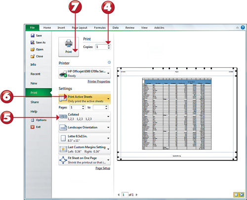
![]() Type the number of copies you want to print in the Number of Copies field, which defaults to 1.
Type the number of copies you want to print in the Number of Copies field, which defaults to 1.
![]() If you want the printed pages to be collated, click the Collate drop-down to set that option.
If you want the printed pages to be collated, click the Collate drop-down to set that option.
![]() In the Settings group, click either Selection (only selected cells), Active Sheet(s) (currently sheets), or Entire workbook (all worksheets and chart sheets).
In the Settings group, click either Selection (only selected cells), Active Sheet(s) (currently sheets), or Entire workbook (all worksheets and chart sheets).
![]() Click the Print button to send your printout to the printer.
Click the Print button to send your printout to the printer.
![]()
Tip: Quick Printing
![]()
You can add the Quick Print command to your Quick Access Toolbar. This allows you to print your entire worksheet without going to the Backstage View. But Revisit Chapter 1 “Working with the Excel User Interface” for a refresher on how to add commands to the Quick Access Toolbar.

