
Raman spectroscopy for biological identification
T.J. Ronningen, J.M. Schuetter, J.L. Wightman, A. Murdock and A.P. Bartko, Battelle Memorial Institute, USA
Abstract:
Advancements in phenotypic identification technologies have overcome some limitations of currently deployed genomic-based systems for species-level biological identification. At the forefront of these advancing technologies, Battelle is applying Raman spectroscopic techniques to rapidly detect and identify prokaryotes and pathogens. Raman spectroscopy has been used for a variety of chemical detection and identification applications but has not been readily utilized for biological pathogen identification. Because the spectra of biological pathogens are exquisitely complicated, spectral features are exceedingly difficult to assign to specific unique molecular bonds within the biological material. However, biological pathogen identification is possible if the subtleties are carefully measured.
Key words
Raman spectroscopy; rapid microbial method; biological identification; optics; multivariate analysis; linear discriminant analysis; support vector machine
11.1 Introduction
Raman identification relies on the detailed analysis of the phenomenological response that results from the phenotypical and structural pathogen characteristics. Bacteria from the Bacillus genus were selected to demonstrate this identification technology. The species consist of genetic descendants of Bacillus cereus and include Bacillus thuringiensis, anthracis and cereus. Statistical analysis of the spectral signatures measured from individual cells of these species shows that the probability of separation is high and can be accomplished using a step-wise process. Lastly, statistical analyses of bacteria that have undergone gamma irradiation deactivation show that the organisms are easily differentiable from the native form. The spectral differences, with respect to the native viable species, suggest structural changes result from the gamma irradiation process. These structural changes may contribute to a further understanding of the phenomenological spectroscopic response from biological systems.
B. anthracis. the causative agent of anthrax, is a gram-positive rod-shaped organism. Virulent forms of B. anthracis contain two plasmids that are referred to as pXO1 and pXO2. The closest genetic relatives of B. anthracis are B. thuringiensis and B. cereus. B. cereus is a common bacterium found in soil. B. cereus can infect humans; however, it is typically not considered to be lethal. The spore form of B. thuringiensis is commonly used as an insecticide to control gypsy moths.
B. cereus, B. thuringiensis and B. anthracis are typically distinguished by genetic analysis of their respective plasmids, as their genomes are largely identical. Differential protein expression and plasmid composition also give rise to distinctive phenotypic differences that can be reliably measured using Raman spectroscopy. Raman spectroscopy is an analytical, materials characterization technique that has recently been adapted and assessed for its capabilities in the field of biology.
Because of improvements in lasers, photo detectors, optics and statistical classification algorithms, the historical problems associated with biological materials analysis – autofluorescence, low Raman sensitivity and spectral discrimination – have been overcome. These advances have enabled the identification of cells at the species level and, to some extent, at the strain level.
Differentiators within biological Raman spectra are primarily attributed to subtle differences in the composition and structure. Although biochemical information can be interpreted broadly as being representative of classes of chemical bonds that exist as resonances within the spectrum, specific spectral assignments are difficult because of the exquisitely complex nature of the organism. Therefore, Raman spectra are analyzed as phenomenological signatures rather than attempting to assign Raman resonances to specific bonding schemes, concentrations and geometries. However, some Raman resonances in the measured spectra can be specifically assigned to chemical bonds. For instance, the aromatic ring structure of the tyrosine and tryptophan amino acids results in a spectral resonance within the approximate range of 995 to 1004 cm−1. Moreover, the carbon–hydrogen and nitrogen–hydrogen spectral resonances occur at 2900 cm−1 and 3200 cm−1, respectively.
While it is beneficial to understand and assign features, it is not necessary to chemically interpret the full spectrum in order to make use of it for species-level classification. Raman spectra can be employed as phenomenological signatures for the purpose of classification. However, it is still necessary to understand and capture phenotypic variability resulting from environmental factors (extensive properties). Extensive properties, such as temperature, age and available nutrients, modulate the expression of organism composition and structure (intensive properties) and, correspondingly, result in small spectral differences that must be taken into account during the spectral analysis.
Extensive organism properties are exhibited in the Raman spectra as spurious and modulated intensity variations. Although irksome, these variations can be tempered and accounted for through appropriate algorithmic techniques, signal to noise optimization and careful optical system design.
The details of the algorithmic inclusion of extensive organism properties will be described in detail in a future manuscript. However, the thesis of this work will delineate the capability to discern species-level identification, based on the intensive properties, of genetic descendants of B. cereus.
11.2 Experimental methods used to capture intensive variability
11.2.1 Bacterium sample preparation
Numerous methods have been developed to identify B. anthracis in case of a bioterrorist attack. B. anthracis is classified as a Biosafety Level 3 (BSL-3) organism and thus must be handled under strict safety specifications. Because of these restrictions, several closely related organisms have been used as simulant organisms during the development and testing of identification methods. Three of these organisms, Bacillus anthracis Sterne strain (BaS), Bacillus cereus (Bc, ATCC #14579) and Bacillus thuringiensis var. Israelensis (Bti) have been selected for this study to act as surrogates for B. anthracis and demonstrate the capability to differentiate between closely related species using Raman spectroscopy. Bc and Bti are close genetic neighbors of B. anthracis and are almost indistinguishable to most assays.1 However, both are Biosafety Level 1 (BSL-1) organisms. BaS is a strain of B. anthracis that is missing the pXO2 plasmid, making it non-virulent. It is used as a vaccine strain in animals. BaS is a Biosafety Level 2 (BSL-2) organism. Many BaS spores and cells were subject to gamma irradiation prior to study in order to determine the effects of the deactivation process. All strains were obtained from Battelle stocks.
Stock suspensions of BaS, Bc and Bti were streaked onto Tryptic soy agar and incubated for 16–24 hours at 37 °C to produce isolated colonies. An isolated colony was used to inoculate 50 ml of Nutrient Broth in a 250 ml flask. The flask was shaken overnight at 37 °C at 200 revolutions per minute (rpm). To produce working cultures for sample preparation, 50 μl of overnight culture was pipetted into 400 ml of Modified G Broth in a 4l flask. The flasks were incubated at 37 °C with shaking at 200 rpm for 72 hours to allow sporulation. The cultures were then heat-shocked at 60 °C for 2 hours in an incubator shaker at 37 °C, 200 rpm. Both pre- and post-heat-shocked samples were plated to assess percent sporulation. Wet mounts of the cultures were examined under a light microscope using an oil immersion lens and the dark field to confirm the presence of spores. The cultures were washed by centrifugation and resuspension in sterile distilled water (SDH2O) a total of three times.
A second suspension of BaS was rendered non-viable by gamma irradiation. A 0.1 ml aliquot of pre-inactivated product was plated onto a trypticase soy agar (TSA) plate. The remaining 500 ml stock suspension (approximately 106 colony forming units/ml) was irradiated with a 60Co source with a fluence of 42.8 kGy for 155 minutes. Afterwards, ten TSA plates were inoculated with 0.1 ml inactivated product. An uninoculated plate was the negative control. All were incubated at 37 °C for 72 days. The positive control TSA plate showed confluency. The TSA plates with inactivated product and the negative control showed no growth, verifying BaS non-viability.
Washed biological suspensions were diluted either 1:100 or 1:50 in SDH2O prior to sample preparation. A 5 μl drop of diluted slurry was placed on the centerof an aluminized glass slide. The slide was placed on a heat block resting on an orbital shaker. The drop of suspension was allowed to dry at 55 °C for 1 minute while shaking at approximately 60 rpm. The dried droplet was analyzed within 72 hours of preparation.
Despite the care and handling of the biological suspension, samples generally have a mixture of target materials, cell debris, grown media and insoluble contaminants. Moreover, samples that are collected from the environment are typically laden with particulate matter that must be algorithmically separated from the targeted biological materials of interest.
11.2.2 Raman micro-spectroscopy
Raman spectra were collected using a Battelle designed system that automatically collects microscope images of the sample, identifies particles within those images and collects the spectra of particles of interest. The process, established by Battelle for the detection and identification of microbiological materials, is entitled the Resource Effective Bio-identification System (REBS). REBS combines high numerical aperture micro-Raman spectroscopy with the means to determine the organism’s species-level identity. The system is controlled by Battelle proprietary software, running on a standard personal computer, which interfaces with all hardware and electronic elements and also carries out image and spectral analysis. The system uses three Newport stages – two VP-25XA for horizontal motion and one VP-5ZA for vertical – to adjust the sample position. These stages have a resolution below 0.1 μm and repeatability below 0.3 μm in order to study target particles as small as 0.3 μm.
For imaging, the system uses a dark-field ring illuminator and a 100 ×, 0.95 NA Olympus microscope objective. The illuminated field of view is an 85 μm diameter circle. The image is recorded using a Charge Coupled Device (CCD) camera and analyzed using edge detection to identify any particles present. The system then repositions the sample in order to record the Raman spectrum of each particle selected. The particles can be selected based on their size, shape and illumination properties. For this study, all particles with an equivalent diameter of 0.75-5.0 μm were selected. This size range includes single cells of the Bacillus targets and small clusters of targets.
Confocal Raman spectra are measured using a top-illumination configuration; that is, the excitation laser and the scattered photons pass through the imaging objective above the sample. The excitation laser is a diode laser in the 640 nm spectral region. The laser is a proprietary Battelle design that incorporates a 250 mW laser diode and a grating stabilization so that the output has a spectral width less than 0.1 nm (full width at half maximum). The laser illumination spot on the sample is 1.0 μm in diameter and the laser power is limited to 12 mW in order to avoid heat damage to the target particles.
The Raman scattered photons are separated from the reflected and Rayleigh scattered photons using a Semrock RazorEdge, 45° dichroic filter followed by a RazorEdge long-pass filter, allowing photons within 150 cm−1 of the excitation radiation to reach the spectrometer. The spectrometer consists of a Headwall Raman Explorer spectrograph with a 10 μm slit aperture at the entrance and an Andor iDus CCD for detection. The spectrograph grating is customized to match the laser wavelength and disperse Raman shifted radiation across the range 1003150 cm−1 over the 1024 CCD sensor columns. The average spectral resolution is 3 cm−1. The dispersion of the spectrometer is calibrated using at least 20 emission lines from a low-pressure neon lamp. The positions of the lines are fitted, using a third order polynomial, against the National Institute of Standards and Technology atomic transition wavelength to obtain calibration coefficients. The laser wavelength is calibrated by recording the Raman spectrum of polystyrene and calculating the best fit to the 11 standardized peaks.2 Polystyrene validation measurements are performed on a daily basis.
Particles selected from the field of view are successively positioned under the excitation laser. The field of view is refocused after each particle is processed in order to ensure optimal signal collection. Each spectrum is recorded as a series of replicate spectra to avoid CCD saturation, for a total of 2 min. If only biological materials are being targeted, an initial spectral filter is applied to the first replicate. This filter uses the presence, or absence, of a carbon–hydrogen (CH) molecular bond stretch feature at 2850 cm−1 to determine whether to continue collecting a spectrum. Any spectra that lack a CH stretch feature are not analyzed further. All biological materials examined to date have possessed CH spectral features.
11.3 Multivariate spectral analysis methods
11.3.1 Spectral analysis
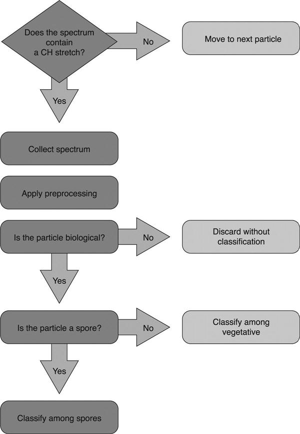
The procedure for processing each spectrum to determine the particle classification is shown diagrammatically in Fig. 11.1. This procedure is designed to eliminate inorganic and/or non-biological particles prior to classification. Next, the classification separates sporulated bacteria from vegetative bacteria and then assigns a species-level classification. Information on each of the steps is provided below.
11.3.2 Data processing
The spectral data are collected in a series of eight sequential, replicate measurements for each particle analyzed. The collection of replicates allows the spectral integration time to be increased without risking CCD saturation. The replicates are also intercompared in subsequent steps in order to identify and remove noise features. The replicate data are then summed into a single spectrum(e.g. the top spectrum in Fig. 11.2). After summation, noise peaks that arise from CCD signal fluctuations and cosmic spikes are detected and removed. Next, the baseline signal is removed using a modification of the rolling-circle filter.3,4 The spectrum is then mapped onto a nominal wavenumber grid using the spectrometer calibration and a cubic spline interpolation. This is the second stage illustrated in Fig. 11.2.
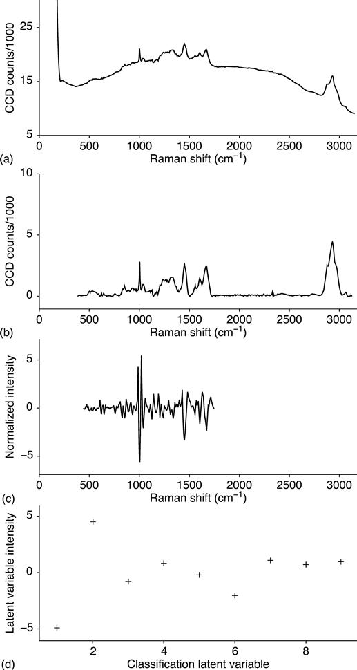
Subsequently, data from some spectral regions that are unimportant are discarded. These regions have been empirically determined not to contain information useful for biological species-level identification. Spectral data between approximately 400 and 1800 cm−1 are retained. This region is the ‘fingerprint’ region for Raman spectra. The smoothed second derivative of the spectral fingerprint region is then calculated using an 11-point Savitzky–Golay filter. Normalization is applied that adjusts the intensity of each data point so that the entire spectral fingerprint region has the same Euclidean length. This is the third stage illustrated in Fig. 11.2.
Finally, prior to each filter or classification step, a dimension reduction is performed using Partial Least Squares (PLS)5 so that each spectrum is then represented by nine values, each associated with a latent variable. These nine values are used for species classification. This is the final stage illustrated in Fig. 11.2, and this dimension reduction is discussed further below.
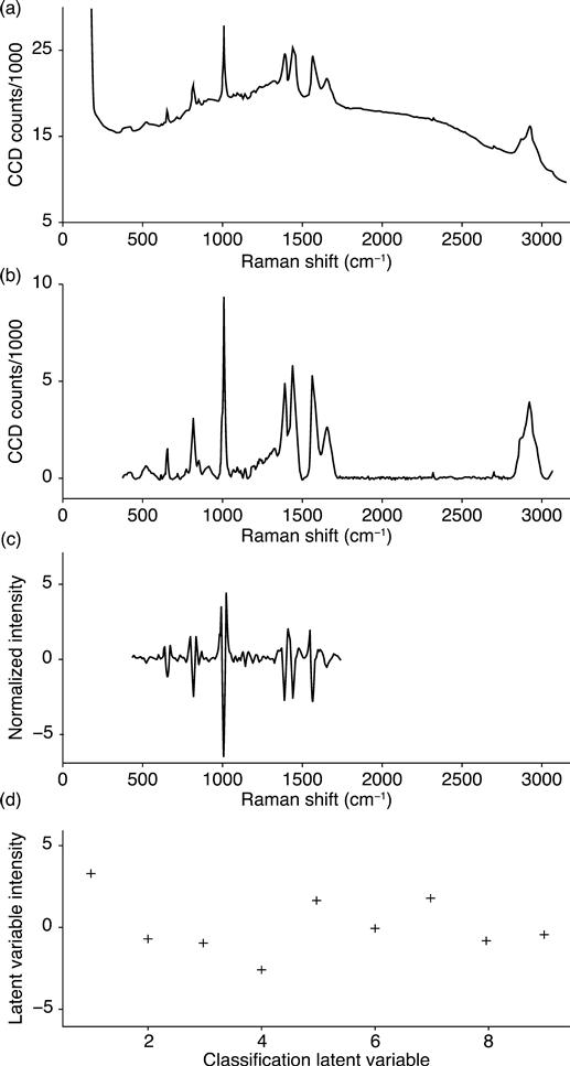
Figure 11.3 presents a second example of the data processing procedure. Both Fig. 11.2 and Fig. 11.3 are spectra of the BaS organism. The spectra differ because the cell in the latter has sporulated.
11.3.3 Dimension reduction
It is common in chemometric and other data analysis methods to reduce the dimensionality of the data. This reduction is often achieved by using a linear combination of the original variables to generate a new set of variables. In geometric terms, this is a coordinate system transformation. The linear combinations used for this transformation are referred to as loading vectors because they quantify the relative contribution from each original variable, that is, Raman shift space captured on the pixels of the CCD detector. The new sets of variables are referred to as latent variables because they can reveal information that is masked in the original coordinate system. A full coordinate system transformation would require that the number of latent variables be equal to the number of original variables. Chemometric methods reduce the number of latent variables to those that carry the most significant information and discard the less significant variables.
There are several reasons for reducing the dimensionality of the spectral data prior to classification. First, it is difficult to adequately train algorithmic classifiers that use a large number of variables. A correspondingly large amount of training data is required so that the significance of each variable can be determined. Also, it is often the case that not all of the variables, that is, all of the spectral regions, are equally significant in biological species-level classification. Regions that are not significant to classification can be removed entirely, as is done when spectra outside the fingerprint region are removed, or have their significance reduced by limiting their contribution through the loading vector. Finally, if any of the variables are highly correlated, it is valuable to remove this correlation and workinstead with latent variables that are not correlated. Spectral data tend to have high correlation across variables because a single spectroscopic peak is typically spread across multiple CCD pixels. All of the data in these pixels rise and fall together (i.e. are strongly correlated).
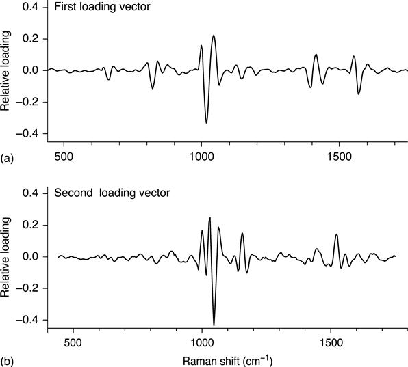
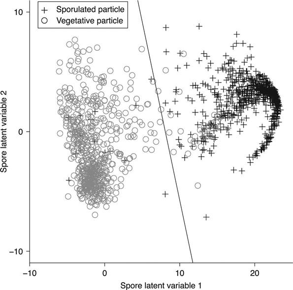
PLS dimension reduction achieves these objectives by determining which spectral features are most strongly correlated with the classification. As an example, the PLS reduction associated with separating sporulated bacteria from vegetative bacteria is illustrated in Figs 11.4 and 11.5. Figure 11.4 depicts the two loading vectors associated with the two retained latent variables. The first loading vector places emphasis on the spectral features at 658, 822, 1013, 1395 and 1572 cm−1. These are the spectral features associated with calcium dipicolinic acid (CaDPA),6 which is a major component of the spore coating. These features also stand out as the main differences between the spectra of a vegetative BaS cell in Fig. 11.2 and a sporulated BaS cell in Fig. 11.3. Figure 11.5 depicts the distribution of the spectra in this new, two-dimensional coordinate system. The spectra associated with sporulated cells cluster strongly on the right hand side of the graph, indicating that the classification information has been captured well by the first latent variable.
Moreover, the PLS dimension reduction approach is sensitive to the significant spectral components of the training set and weights their significance. The weighting helps to alleviate spurious signature elements that are the result of extensive properties or environmental variability of the organism that are not related to the species identification.
11.3.4 Classification techniques
Once the spectra have been processed and the dimensions reduced, it is necessary to classify them based on the values of the latent variables. Classification is based, fundamentally, on the similarity of spectra that arise from the same class. In the mathematical representations, this similarity causes the spectra from one species to cluster tightly together in the latent variable space and to be separated from the spectra of another class. This is illustrated in Fig. 11.5, where spectra of sporulatedcells cluster together on the right hand side while vegetative cells cluster to the left. A classification algorithm is used to automatically determine the class to which a test spectrum is most similar. Both linear discriminant analysis (LDA) and support vector machine (SVM) classification7 techniques are used in this analysis.
LDA classification assumes that the distribution within a class is a normal (Gaussian) distribution. The training spectra for a class are fitted to a multidimensional Gaussian, and the parameters derived from this fit are used to classify test spectra as either inside or outside this distribution. The line in Fig. 11.5 is the linear discriminant boundary that separates sporulated from vegetative cells.
SVM classification techniques analyze class distributions in order to find the optimal boundaries between classes. The points or class members that define these boundaries are the most significant data points–unlike LDA, where the points near the center of the class distribution are most significant. SVM does not assume a form for the distribution of the class members and is therefore better able, compared with LDA, to separate classes along irregular boundaries. Because SVM is most sensitive to data points along the boundaries, it sometimes requires a larger data set than other classification methods such as LDA.
11.4 Species-level biological identification results
Table 11.1 lists the number of spectra measured for this study in each classification category. The non-biological contaminants on the slide are designated as NT for ‘not a target’. Two types of BaS samples were measured, one with viable cells and the other with irradiated cells. In order to determine whether the irradiation process led to any changes in the spectral signature, the two types of cells were treated separately.
Table 11.1
Number of species in the spectral data set for each organism type
| Species | Number of spectra |
| BaS, irradiated | 509 |
| Bc | 138 |
| BaS, viable | 283 |
| Bti | 386 |
| NT | 903 |
| All | 1973 |
In order to measure classification performance, it was necessary to train the classification algorithms with a training set and then determine the performance with a test set. The test set must be kept separate from the training set in order to avoid overestimating the performance. It is also desirable to avoid biasing the results by a particular separation of training and testing data. In order to avoid this source of bias, 1000 distinct combinations of testing and training data were generated. For each combination of CH, biological and spore values (six total combinations), 1000 train/test sets were randomly generated from combinations of the measured spectra. In each case, the measured spectra from each species subclass was evenly split into the test or training group.
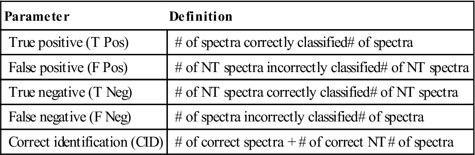
The performance at each filter stage, and for each test/train set, was captured by a confusion matrix. A confusion matrix compares the classification results with the established truth for each spectrum. The confusion matrices for each test/train set were averaged to obtain an unbiased confusion matrix, representative of the overall performance. These average confusion matrices are presented below. Each confusion matrix was also summarized by the five parameters defined in Table 11.2.
Table 11.2
Filter performance parameters for organic/inorganic, biological/non-biological, spore/non-spore and species-level determinations
| Parameter | Definition |
| True positive (T Pos) | |
| False positive (F Pos) | |
| True negative (T Neg) | |
| False negative (F Neg) | |
| Correct identification (CID) |
11.4.1 Spectral classification procedure
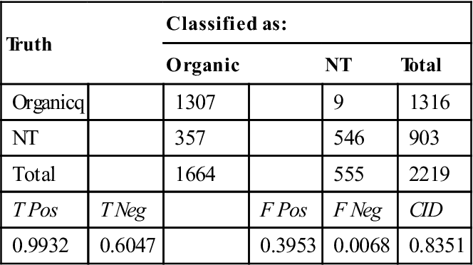
The first filtration step, as indicated in Fig. 11.1, is the determination of organic content using the CH stretch filter. This filter was implemented with a peak detection algorithm so that the result can be obtained quickly. The confusion matrix for the CH stretch filter is presented in Table 11.3. The high true positive rate of 99.32% was most critical for this filter, since a biological particle rejected at this stage has no chance of being identified correctly. The relatively high false positive rate of 39.53% indicates that unnecessary time was used to collect the spectra of NT material, but a significant amount of time was saved by rejecting the other 60.47% of the NT particles.
Table 11.3
Organic/inorganic determination performance based on CH stretch filter results for all particles spectrally measured
| Truth | Classified as: | ||||
| Organic | NT | Total | |||
| Organicq | 1307 | 9 | 1316 | ||
| NT | 357 | 546 | 903 | ||
| Total | 1664 | 555 | 2219 | ||
| T Pos | T Neg | F Pos | F Neg | CID | |
| 0.9932 | 0.6047 | 0.3953 | 0.0068 | 0.8351 | |
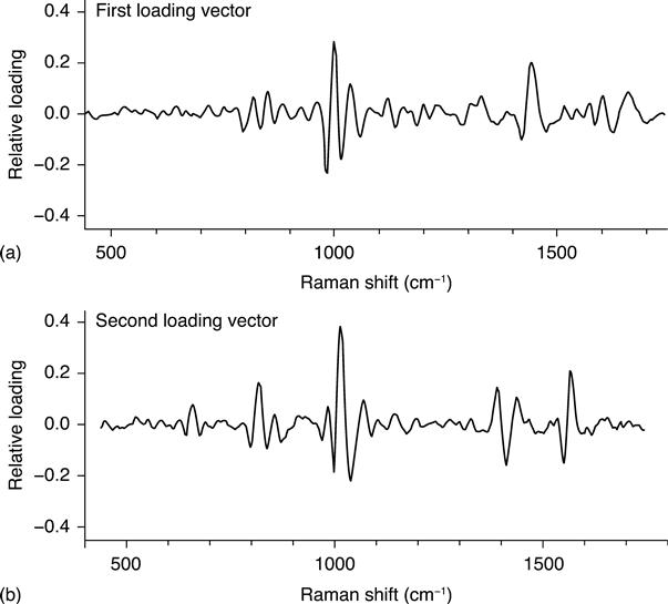
The second stage of filtration separates biological particles from non-biological particles. This filter uses a PLS reduction to two latent variables and a LDA classifier. The two PLS loading vectors are illustrated in Fig. 11.6. These vectors emphasize spectral features near 1004, 1445 and 1655 cm−1 that originate, respectively, from phenylalanine (ring breathing mode), CH2 and CH3 deformationmotions and the Amide I band (N–C = O stretching). These are relatively strong features that are shared by all biological particles, including viral and protein agglomerations.
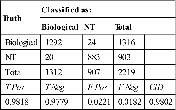
The distribution of test spectra in the two-dimensional, latent variable space of the biological filter is illustrated in Fig. 11.7. The LDA separation boundary is indicated by the line. The confusion matrix for this filter is presented in Table 11.4. The true positive, 98.18%, and the true negative, 97.79%, are high for this filter, indicating that it efficiently distinguished the two classes of material. Note that the NT spectra classified by the CH stretch filter as NT were not analyzed by the biological filter but instead remained classified as NT.
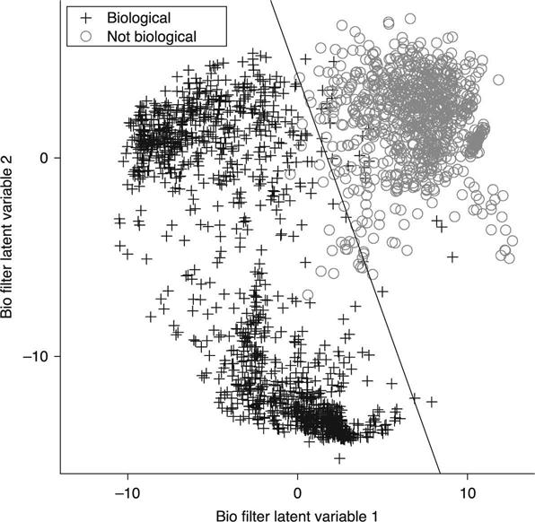
Table 11.4
Biological/non-biological determination performance based on the LDA of the spectral space reduced to two latent variables
| Truth | Classified as: | |||
| Biological | NT | Total | ||
| Biological | 1292 | 24 | 1316 | |
| NT | 20 | 883 | 903 | |
| Total | 1312 | 907 | 2219 | |
| T Pos | T Neg | F Pos | F Neg | CID |
| 0.9818 | 0.9779 | 0.0221 | 0.0182 | 0.9802 |
Spectra that were determined to be biological are then classified in two stages. The first stage of classification separates biological particles that are sporulated from those that are not. For this test set of Bacillus cells, non-sporulated particles are either vegetative or NT, but the filter also classifies gram negative bacteria, pollen, yeast, viruses or proteins as being non-sporulated. The spore filter usesPLS reduction to two dimensions and a LDA classifier. The loading vectors and the distribution of spectra in the space of the two latent variables are illustrated in Figs 11.4 and 11.5, respectively.
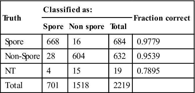
The confusion matrix for the spore filter is presented in Table 11.5. As with the biological filter, the separation performance was excellent, with 97.79% of sporulated particles classified correctly and 95.39% of vegetative cells classified correctly. Division of the particles into sporulated and vegetative classes allows the final stage of the classification algorithm to focus solely on features that separate spectra within their respective species.
Table 11.5
Spore/non-spore determination performance based on the LDA of the spectral space reduced to two latent variables
| Truth | Classified as: | Fraction correct | ||
| Spore | Non spore | Total | ||
| Spore | 668 | 16 | 684 | 0.9779 |
| Non-Spore | 28 | 604 | 632 | 0.9539 |
| NT | 4 | 15 | 19 | 0.7895 |
| Total | 701 | 1518 | 2219 | |
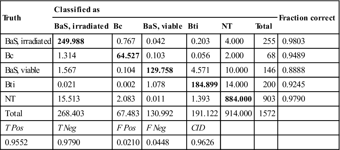
The results of the spore filter determined whether a spectrum was identified using a spore library classifier or a non-spore library classifier. These classifiers have distinct training sets, but both were found to be optimized using nine PLS latent variables. Both classifiers use a SVM classification algorithm. The confusion matrix for the separate classifiers is presented in Table 11.6 and the overall confusion matrix for this identification approach is presented in Table 11.7. The irradiated BaS spores and vegetative cells showed some misclassification at the spore filter, but, for the most part, the species was identified correctly. The vegetative BaS and Bti misclassification primarily takes place at the stage ofthe biological filter, where some cells were incorrectly classified as NT. The interspecies confusion was minimal, and therefore the overall correct identification rate was quite strong at 96.26%.
Table 11.6
Species-level classification performance based on the support vector machine analysis of separate spore and non-spore spectral libraries
| Truth | Classified as: | Fraction correct | |||||||||
| BaS spore, irradiated | BAS veg, irradiated | Bc spore | Bc veg | BaS spore, viable | BaS veg, viable | Bti spore | Bti veg | NT | Total | ||
| BaS spore, irradiated | 99.525 | 5.999 | 0.432 | 0.001 | 0.042 | 0.000 | 0.001 | 0.000 | 1.000 | 107 | 0.9301 |
| BaS veg, irradiated | 10.000 | 134.464 | 0.000 | 0.334 | 0.000 | 0.000 | 0.000 | 0.202 | 3.000 | 148 | 0.9085 |
| Bc spore | 0.967 | 0.000 | 22.031 | 0.000 | 0.002 | 0.000 | 0.000 | 0.000 | 1.000 | 24 | 0.9180 |
| Bc veg | 0.000 | 0.347 | 0.000 | 42.496 | 0.000 | 0.101 | 0.000 | 0.056 | 1.000 | 44 | 0.9658 |
| BaS spore, viable | 0.524 | 0.013 | 0.046 | 0.000 | 104.468 | 0.985 | 3.962 | 0.002 | 1.000 | 111 | 0.9412 |
| BaS veg, viable | 0.028 | 1.002 | 0.003 | 0.055 | 1.885 | 22.420 | 0.084 | 0.523 | 9.000 | 35 | 0.6406 |
| Bti spore | 0.017 | 0.000 | 0.000 | 0.000 | 0.636 | 0.000 | 98.347 | 0.000 | 2.000 | 101 | 0.9737 |
| Bti veg | 0.000 | 0.004 | 0.000 | 0.002 | 0.000 | 0.442 | 0.000 | 86.552 | 12.000 | 99 | 0.8743 |
| NT | 3.997 | 11.516 | 0.001 | 2.082 | 0.002 | 0.009 | 0.000 | 1.393 | 884.000 | 903 | 0.9790 |
| Total | 115.058 | 153.345 | 22.513 | 44.970 | 107.035 | 23.957 | 102.394 | 88.728 | 914.000 | 1572 | |
| TPos | T Neg | FPos | F Neg | CID | |||||||
| 0.9552 | 0.9790 | 0.0210 | 0.0448 | 0.9506 | |||||||
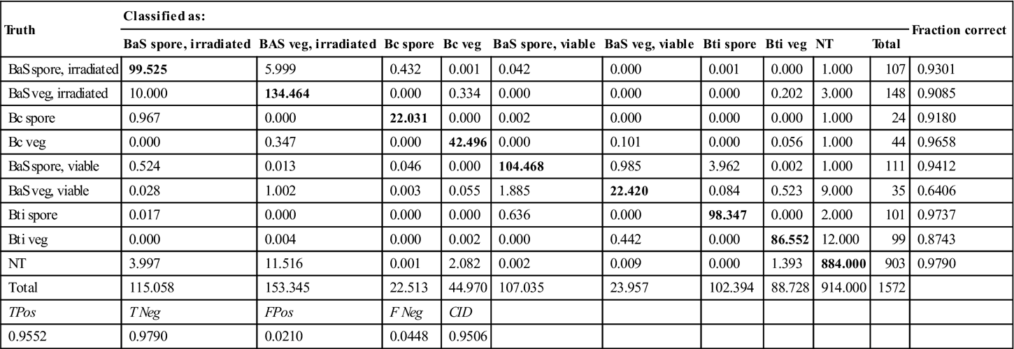
Table 11.7
Species-level classification performance based on the combined spore and non-spore classifications shown in Table 11.6
| Truth | Classified as | Fraction correct | |||||
| BaS, irradiated | Bc | BaS, viable | Bti | NT | Total | ||
| BaS, irradiated | 249.988 | 0.767 | 0.042 | 0.203 | 4.000 | 255 | 0.9803 |
| Bc | 1.314 | 64.527 | 0.103 | 0.056 | 2.000 | 68 | 0.9489 |
| BaS, viable | 1.567 | 0.104 | 129.758 | 4.571 | 10.000 | 146 | 0.8888 |
| Bti | 0.021 | 0.002 | 1.078 | 184.899 | 14.000 | 200 | 0.9245 |
| NT | 15.513 | 2.083 | 0.011 | 1.393 | 884.000 | 903 | 0.9790 |
| Total | 268.403 | 67.483 | 130.992 | 191.122 | 914.000 | 1572 | |
| T Pos | T Neg | F Pos | F Neg | CID | |||
| 0.9552 | 0.9790 | 0.0210 | 0.0448 | 0.9626 | |||
11.4.2 Biological deactivation by irradiation
The differentiable spectra between irradiated and viable BaS samples shows that the irradiation process changes the organism in a measurable and consistent way. However, it remains challenging to attribute changes caused by the irradiation process. It is clear that spore lysis is not the dominant deactivation mechanism, because neither the particle morphology nor the malachite-green staining response, examined in a separate study, changes (data not shown).
An examination of the spectra shows that the gamma irradiation-induced changes occur throughout the spectral space. As seen in Fig. 11.8, the difference spectrum for vegetative BaS shows variances across the spectral fingerprint region. The difference spectrum is calculated by subtracting the average viable target spectrum from the average irradiated target spectrum. The difference spectrum shows where the spectral responses are prevalent or diminished with respect to each other.
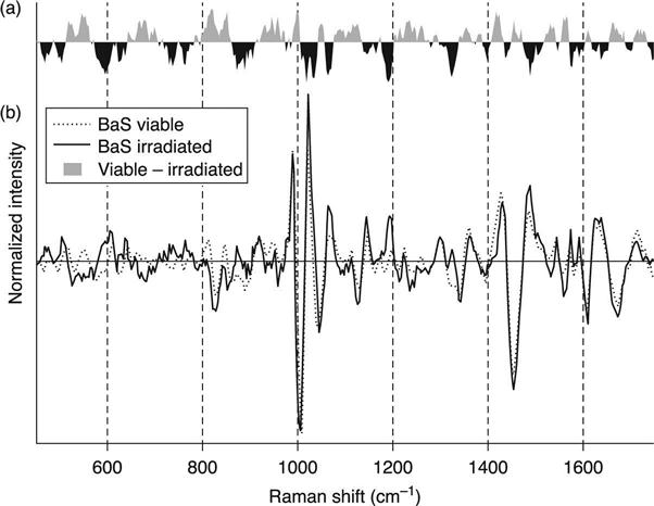
There are differences that can be attributed to regions of known molecular composition. For instance, the 1000 cm−1 region of the spectra is known to contain phenylalanine. The difference spectra show a complex differential between the viable and irradiated exemplar spectra in this region. Similarly, changes at approximately 1425 cm−1 may be attributed to Amide I bands or similarly polarizable molecular bonds. These areas in the spectra are well known and, potentially, may indicate how the gamma deactivation alters the organism. These findings will be shared in a future publication. Nonetheless, the alterations of the organisms are clear and consistent in the spectral space. Therefore, spectral library development cannot replace the spectral signature of a viable organism with its irradiated counterpart.
11.5 Conclusions
Battelle Memorial Institute has developed and tested a microbial identification system that is based on Raman spectroscopy (REBS) and has proved that it is well suited to detect and identify closely related individual Bacillus cells with greater than 96% probability of correct identification at the species level. Detailed assessments of Battelle’s approach have shown its applicability to security, defense and industrial applications, because results have shown that differentiationbetween near-neighbor Bacillus species is possible through Raman spectroscopic methods. Experimental studies also show that the technology can provide identification information faster than currently available technologies that utilize reagents or consumables. Having actionable information, in minutes rather than hours, will enable faster decisions about local environmental threats in security applications and provide heightened manufacturing process awareness in industrial applications. Ultimately, decreasing the time to an actionable result will lead to a safer society and more economical products.
Testing and evaluation strategies for rapid spectroscopic biological identification of systems typically use attenuated or deactivated pathogens, primarily for safety and convenience. Until recently, heat-killed or gamma-irradiated biological agentlike organisms have been used in testing and evaluation because the states of the killed material seldom change the outcome of genomic-based identification processes. Genomic-based identification processes target genomic content rather than organism integrity or completeness. Phenotypic-based identification systems rely on the pathogen’s structural integrity, which is often lost during neutralization. Therefore, heat-killed or gamma-irradiated organisms are not ideal for testing phenotypic methods such as spectroscopic identification. Nonetheless, phenotypic identification of irradiated organisms remains possible; however, the results of the testing and evaluation should be interpreted carefully, and a distinction made between viable and dead organisms.
11.6 Acknowledgments
The authors gratefully acknowledge R. Black, T. Petrel, K. Sadeski, L. Lynch, R. Daly, G. Assenheimer, D. Daugherty, R. Marzette, A. Schimmoeller, D. Jackson, R. Shoaf, G. Oliver, K. Guspan, C. Fortney, D. Mooney, C. Dingus, F. Todt, J. Regensburger, B. Ray, L. Aume, S. Rust, C. A. Morrow, B. Ross, L. P. Vassy and many other colleagues whose contributions to this effort were essential. Finally, the team gratefully acknowledges the vision and financial support from Battelle Memorial Institute.