CHAPTER 11
Tape Replay
The Return of Tape
When I was writing the first edition of Small Signal Audio Design in 2009, and indeed the second edition in 2015, it never occurred to me to include the technology of magnetic tape. It was gone and showed no signs of coming back. However, there were several vintage multi-track tape recorders displayed at the Paris AES Convention in June 2016, and reel-to-reel tape machines are now (2019) enjoying a revival. Perhaps that was inevitable after the vinyl revival, but few people predicted that cassette tapes would also come back to haunt us, and now they have. [1] Quite suddenly, there is a need for new tape machines to play back old formats. I would have bet a lot of money that the one format which would never come back would be the dreadful eight-track cartridge. I would have lost that money, because it’s happening at the time of writing in 2019; see [2]. Wax cylinders have already been revived once, by The Men Who Will Not Be Blamed For Nothing, though they might well be blamed for that. [3] It seemed unlikely the experiment would be repeated, but see Chapter 9 …
Another format that is probably, and this time regrettably, not coming back is the Elcaset [4] which looked like an enlarged compact cassette and used ¼-inch tape running at 3.75 ips. An important feature was that a tape loop was pulled out of the Elcaset by the transport, reducing the effect of imprecise cassette mechanics. Much better quality compared with compact cassette was easily obtainable, and three-head operation was standard. The Elcaset was a collaboration between Sony, Panasonic, and Teac, introduced in 1976. Unfortunately, at this time, compact cassette quality was rapidly improving due to the introduction of chromium tape and Dolby, and the system failed utterly in the marketplace, which is perhaps rather a pity, as it was technically very sound, and it was abandoned in 1980. And despite what I said at the start of this paragraph, at time of going to press, I discover that in 2017, Jeremy Hieden released an album called Blue Wicked on every obsolete format he could find, including Elcaset, making it the first ever pre-recorded album on Elcaset. Apparently only Laserdisc defeated him. (Note that Elcaset is the correct spelling, not Elcassette.)
Tape is unmistakably coming back, like it or not, and so I have added this chapter. Tape technology is complicated, even if we confine ourselves to the replay part of the process, which I think is reasonable given the small number of people who are going to be designing new tape recorders from scratch and a perceptible trend towards playback-only tape machines for pre-recorded tapes. I will only go into the recording side where it is necessary to understand something on the replay side. Even so, a really comprehensive book on tape replay would be at least as long as Electronics for Vinyl [5], which has 327 pages just on vinyl replay. If it comprehensively covered recording and tape transport as well, I think it would be a mighty tome. Wikipedia has some very good articles on tape technology, and I will give frequent references to these to keep the length of this chapter under control.
I should perhaps confess that while I have designed many amplifiers and many mixing consoles, to the point where I have lost count of both, I have only designed one tape recorder, back in the late 1970s. The replay amplifiers were all discrete-transistor technology, with some cunning crosstalk-cancellation (see later). It had no Dolby-B noise-reduction, as licenses to use it were expensive. It was not exactly high-end hi-fi, but it worked all right, and we sold quite a few.
A Brief History of Tape Recording
The first halfway practical magnetic recorder was built in 1898 by Poulsen. It used steel wire as the storage medium. The replay output was too low to be of use until valve amplifiers were introduced around 1909. Wire was later replaced by steel tape, the machines being called Blattnerphones after the inventor, Louis Blattner; it was a difficult medium to handle, and the BBC considered them acceptable for voice but not music. Steel tape was replaced by paper tape coated with ferric oxide in 1930s, and this was in turn replaced by oxide-coated PVC tape. The introduction of AC bias to reduce noise and distortion was a vital step to making tape recorders useful; its history and application are described in the next section.
The Basics of Tape Recording
This section is kept short to allow more room for consideration of the replay electronics. The tape recording process creates varying degrees of magnetisation on the tape by passing audio signal through the windings of the record head in contact with it; this by itself is not a very linear process, but the non-linearity is smoothed over by also applying a bias signal of higher frequency than the audio band being recorded.
The standard tape speeds are: 30 ips, 15 ips, 7.5 ips, 3.75 ips, and 1.875 ips [6], where ips means inches per second; the metric equivalent of cm/sec is rarely used, probably because it results in lots of awkward numbers such as 7.5 ips = 19.05 cm/sec. The faster the tape speed, the better the quality. Thus 1.875 ips is mainly used in compact cassettes [7], which were originally designed for recording dictation, where voice-only quality was acceptable. A lot of development work was required to make the compact cassette capable of producing decent audio. Even slower speeds exist; namely 15/16 ips and 15/32 ips are used in microcassettes [8], and these are just used for voice recording, though that should probably be were, as digital voice recorders are much superior. Higher speeds of 60 and 120 ips were once used for analogue data recorders but have never been used in audio.
The basic setup is shown in Figure 11.1. Frequencies below 100 Hz are frequently boosted to offset losses in the record/replay process. The record head has significant inductance, so to get a level response, it must be driven from a high impedance; using a high-value resistor usually loses too much voltage swing, so an amplifier with a current source output is used. A record head has fewer turns than a replay head and so lower inductance in order to minimise the extent of the problem. The bias signal is summed with the audio signal at the tape head. It is important to prevent the bias signal from being fed into the output of the record amplifier, as it will wreck its linearity or maybe stop it working altogether. This is pretty much universally accomplished by putting a parallel-LC circuit in series with the output of the recording amplifier, as in Figure 11.1. Inductors are relatively uncommon nowadays in electronic circuitry, but here they are still the best option. For example, the Sony TC-A590/A790, introduced in 1996, still used passive LC bias traps; this technology is likely to continue.

Extraordinarily, the use of AC bias (as opposed to crude and unsatisfactory DC bias) goes back to a 1921 patent by Carlson and Carpenter [9], but the technique was forgotten and reinvented several times until being finally and solidly reinvented by Walter Weber in 1941, when a record amplifier went into parasitic oscillation. [10] The bias oscillator normally has a low output impedance, which would shunt away the record amplifier signal, so the bias is injected either through a resistor (R5 in Figure 11.1) or a small capacitor, which may be an adjustable trimmer to set the bias level. The bias signal must be a clean sine wave with no DC component, or noise and/or distortion will be compromised.
Multi-Track Recording
Multi-track recording is the foundation of modern music. There can be anywhere between 4 and 32 tracks on the tape, each of which can be recorded and played back separately, allowing each instrument a dedicated track. The beauty of this is that one mistake does not ruin the whole recording; only a single part need be done again. (And again, and again, if necessary.) The multi-track process is in two basic halves: recording individual tracks (often called “tracklaying”) and mixdown to stereo. One track is usually dedicated to time-code, which in the 4-track case leaves only three audio tracks and makes recording rather difficult. I call 8-tracks the minimum; step forward the Fostex R8. (I have one.)
When recording, normally only one or two parts are recorded at once, though it is quite possible to dedicate five or six tracks to a drum kit or a backing vocal section. The initial sound, whether captured by a microphone or fed in directly from a synthesiser line output, is usually processed as little as possible before committing it to tape; subsonic filtering and perhaps compression or limiting are used, but most effects are carefully avoided because they are usually impossible to undo later. You can easily add reverberation, for example, but just try removing it. It is clearly essential that all the new parts are performed in time with the material already on tape and also that the recording engineer can make up a rough impression of the final mix as recording proceeds. This is done by using the record head as a replay head when it’s not recording, giving a “sync” output that is time aligned with what’s being recorded by another section of the same head. Continually replaying already-recorded material is as important as recording it in the first place. The sync signal is not of the same quality as the replay head output; in particular the HF response will be lacking because the record head has a larger gap than the replay head, but it is quite good enough for keeping musicians playing in time.
When the tracklaying process is complete, it is mixdown time. There are 7, 15 or more separate tape tracks that must be mixed down to stereo. Major manipulations of sound are done at this mixdown stage; since the multi-track tape remains unaltered, the resulting stereo being recorded on a separate two-track machine, any number of experiments can be performed without doing anything irrevocable.
Tape Heads
The electrical characteristics of tape heads are of crucial importance to correct operation, especially in the replay case, where the head inductance has a big effect on the noise performance of the replay amplifier. Figure 11.1 shows a three-head tape recorder. This allows the recorded material to be played back almost immediately to monitor quality and means the record and replay heads can be optimised for their different roles. Cheaper machines have only two heads, the record and replay being done by a single head, and this is pretty much standard for cassette machines, as it is difficult to fit three heads into the openings in a cassette. However, it can be done, and Nakamichi introduced the first three-head cassette decks, the 700 and the 1000 in 1973. Other manufacturers like Sony followed.
It is also possible to fit all three heads into one, giving a record/replay/erase head, sometimes called a Z-combo® head. The record/replay winding are on one half of the magnetic circuit and the erase windings on the other, with an extra pole-piece in the middle. [11] This is suited to use with hard surfaces such as striped film and magnetic cards. It reduces the time delay between erase and record/replay to the minimum.
Tables 11.1, 11.2, and 11.3 show typical head parameters, gathered from several reputable manufacturers. Where the output is not stated, it means the manufacturer didn’t state it, for reasons unknown.
| Function | Inductance mH | DC resistance Ω | Replay output μV |
|---|---|---|---|
| Record | 4 | 13 | n/a |
| Replay | 5 | 15 | 200 |
| Replay | 8 | 15 | 350 |
| Replay | 100 | 140 | |
| Replay | 650 | 650 | 200 |
| Erase | 0.17 | 3.0 | n/a |
| Erase | 1 | 12 | n/a |
| Erase | 1.5 | 18 | n/a |
| Inductance mH | DC resistance Ω | Replay output μV |
|---|---|---|
| 20 | 30 | 350 |
| 100 | 100 | 800 |
| 200 | 190 | 1200 |
| 400 | 350 | 1600 |
| 500 | 315 | 1700 |
| 800 | 640 | 2200 |
| Inductance mH | DC resistance Ω |
|---|---|
| 0.2 | 2.2 |
| 0.8 | 9.0 |
| 8.0 | 45 |
| Inductance mH | DC resistance Ω | Replay output μV |
|---|---|---|
| 20 | 50 | 750 |
| 80 | 110 | |
| 200 | 215 |
| Inductance mH | DC resistance Ω |
|---|---|
| 0.047 | 0.9 |
| 0.28 | 2.2 |
| 0.37 | 2.6 |
| 1 | 10 |
| 2 | 14 |
| 13 | 115 |
The majority of cassette machines are two-head, with the record and replay functions done by the same winding and core; they tend to have a relatively high inductance to get an adequate replay output voltage, but it is generally lower than for ¼-inch replay, where three heads is more common. Likewise, they have narrow gaps suited to replay such as 50 micro-inches rather than the 200 micro-inches used for record-only cassette heads.
Cassette erase heads tend to have a lower inductance than ¼-inch erase heads.
Many examples can be found in the Nortronics catalogue [11], which also has some good general information on tape recording and replay.
Tape Replay
The replay head produces only a small voltage; it is made as large as possible by giving the head coil a large number of turns and consequently a larger inductance than the record head. The replay head has a narrower gap than a replay head.
There are several possible causes of HF loss on tape replay:
- Replay head gap width. At a sufficiently high frequency, the head gap will see a complete cycle of tape magnetisation, and there will be no output. At a much lower frequency, the HF response will begin to droop in at the top of the audio band. This is commonly called gap loss.
- Azimuth error. If the vertical head gap is not exactly at right angles to the direction of tap travel, then the effective gap width is increased, leading to HF loss as described earlier.
- Spacing error. If the tape does not make good contact with the head, for example due to a buildup of oxide on the head face, the effective gap width is again increased, leading to HF loss.
All these issues depend on the relationship between the head gap and the wavelength on tape and so become more significant at lower tape speeds. Simple formulae for calculating the amount of loss are given in [11]. The problems are essentially mechanical and can be controlled by proper head design and regular maintenance and cleaning.
The HF response may also be affected by head resonance, which occurs between the head inductance and its internal stray capacitance, plus the external shunt capacitance from screened cable and added loading capacitors. The frequency must be comfortably above the desired audio HF response. Loading resistors, usually in the range 33 kΩ to 120 kΩ, are used to damp the resonance.
There also are limitations on the minimum frequency that a replay head can reproduce. At low frequencies, the magnetic field on the tape reaches the coil by other paths than just the gap, and partial reinforcements and cancellations put wobbles (that may be up to ±3 dB) in the response; these are sometimes called “head bumps”. Ultimately, the head output drops to zero as the recorded wavelength becomes much longer than the head gap. The longest wavelength is the mean of the lengths of the head pole and the window in the magnetic screening that allows the pole to contact the tape. A good low-frequency response requires a large window, which makes magnetic screening harder. The shape of the laminations in the head pole also affects the low-frequency response. The overall low-frequency loss is frequently called “contour effect”; it occurs only on playback. It is well described in [12].
Unlike vinyl discs, the maximum possible level from a tape is set by magnetic saturation, and there is no need for large amounts of headroom in the replay circuitry to cope with excessive recording levels or transients from scratches. In anything but low-cost machines, it is therefore often convenient to have a first preamplifier optimised for low noise and with a flat response that gets the signal up to a level where it is relatively immune from noise contamination in later circuitry. Equalisation and level control, etc., can therefore be done in separate stages, which simplifies the design process. Tape replay is also free from the subsonic disturbances created by vinyl (unless they are deliberately recorded –see “Auto-Dolby” in what follows), and subsonic filtering is not normally considered necessary.
Tape Replay Equalisation
The signal produced by the replay head is proportional to the rate of change of the magnetic field it sees. The output therefore doubles with each doubling of frequency, and to undo this, the basic replay equalisation is an integrator, i.e. a -6 dB/octave slope. This is modified by making the amplifier response level out at high frequencies, which is in effect HF boost. This compensates for the HF loss mechanisms listed earlier; the lower the tape speed, the greater the losses, and so the lower the frequency at which the gain is made to level out. The frequency is normally quoted as a time-constant, so a 90 μs time-constant T is equivalent to a turnover frequency of 1/T = 1768 Hz. The history of tape equalisation is very complicated [13], but Table 11.6 gives the most common values used.
There is also a levelling-off of gain at the low-frequency end for all speeds except 30 ips, which compensates for bass boost on recording and improves the LF signal-to-noise ratio.

Figure 11.2 Tape-replay equalisation responses from the amplifier in Figure 11.3 for 3.75 and 7.5 ips. The 15 ips response is below the curves shown, while the 1.875 ips response is above.
The equalisation for 3.75 ips is implemented in the replay amplifier of Figure 11.3. C3 performs the integration and is the central component on the equalisation feedback arm. The integration is limited by R2, which causes the gain to level out at HF. Similarly, R3 limits the increase in gain as frequency falls, giving a relative LF cut. R0 sets the overall gain in conjunction with the other feedback components. The gain of this circuit is +35 3 dB at 400 Hz; this frequency is chosen as it is in the “integrating” part of the response and is therefore unaffected by the levelling off at HF and LF.
| Tape speed ips | LF shelf μs | LF shelf Hz | HF shelf μs | HF shelf Hz |
|---|---|---|---|---|
| 30 | None | None | 17.5 | 9095 |
| 15 | 3180 | 50 | 50 | 3183 |
| 7.5 | 3180 | 50 | 50 | 3183 |
| 3.75 | 3180 | 50 | 90 | 1768 |
| 1.875 Fe | 3180 | 50 | 120 | 1326 |
| 1.875 Cr | 3180 | 50 | 90 | 1768 |
The simple Equation 11.1 is frequently given for calculating the equalisation breakpoints. Plug in a preferred value for C3, which will give the desired gain at 400 Hz, and calculate R2 and R3. Unfortunately, the equation is not entirely accurate, as the value of R0 has a significant effect on the response. Your options are then a) do the complex algebra that completely describes the circuit (I’m not aware anyone has done this) or b) determine the approximate value for R2 or R3 with Equation 11.1 and then put the results into a SPICE simulator, where the values of R2 and R3 can be fine-tuned to get exactly the desired break points; this is more my kind of approach to knotty problems. With values of R0 between 100 Ω and 1 kΩ, the corrections to R2 and R3 are unlikely to exceed ±20%. This crude but effective approach only works because the LF and HF levelling-out frequencies are far apart and do not significantly interact; it is not feasible with RIAA phono equalisation where the effects of the time-constants overlap (see Chapter 9).
In the case of 3.75 ips equalisation, the LF time-constant is 3180 μsec, equivalent to exactly 50 Hz. The HF time-constant is 90 μsec, equivalent to 1768 Hz. The calculate-and-tweak process gives R3 = 57k9 and R2 = 1220 Ω. The nearest 1xE24 values are 56 kΩ and 1200 Ω. The value for R2 looks pretty close, but its nominal value is still 1.6% out, and R3 is 3.4% awry. The 1xE96 format for R2 gives 1210 Ω and 0.83% error, while R3 gives 57k6, which has 0.5% error.
The 2xE24 format is usually more accurate than 1xE96, so R3 and R2 were recalculated giving R3 = 110k in parallel with 120k and R2 = 2200 Ω in parallel with 2700 Ω, as shown in Figure 11.3. R2 has 0.64% error in the nominal value and R3 has 0.88% error, which is not much of an improvement, but for both resistors, the effective tolerance is reduced by almost √2. And you don’t have to keep thousands of E96 values in stock.

Figure 11.3 Tape-replay amplifier with 2xE24 equalisation network for 3.75 ips.
| Tape speed ips | R0 | C3 nF | R2 exact Ω | R2A Ω | R2B Ω | R3 exact kΩ | R3A kΩ | R3B kΩ |
|---|---|---|---|---|---|---|---|---|
| 30 | 680 | 10 | 650 | 1300 | 1300 | 1M | – | – |
| 15 | 220 | 33 | 1270 | 2400 | 2700 | 130 | 180 | 470 |
| 7.5 | 100 | 68 | 633 | 1100 | 1500 | 57.9 | 110 | 120 |
| 3.75 | 100 | 68 | 1323 | 2200 | 2700 | 57.9 | 110 | 120 |
| 1.875 CrO2 | 100 | 68 | 1323 | 2200 | 2700 | 57.9 | 110 | 120 |
| 1.875 Fe | 100 | 68 | 1675 | 2700 | 4300 | 57.9 | 110 | 120 |
Table 11.7 shows the results of this process for common tape speeds, with ferric and chrome options for the 1.875 ips cassette speed. The shelving frequencies are all accurate to within ±1%.
The amplifier in Figure 11.3 was designed to keep the impedance of the feedback network as low as possible to minimise Johnson noise and the effect of opamp current noise. First R0 was set to 100 Ω, which means that C4 has to be quite large at 470 μF to avoid it affecting the equalisation accuracy at 20 Hz and below. At the higher tape speeds of 15 and 30 ips, the HF shelving is at so high a frequency that R2 becomes too low and loads the opamp output excessively. For these speeds, R0 is changed to 220 Ω, increasing the general impedance of the feedback network and allowing C4 to be reduced to 220 μF. This means C3 changes to 33 nF to maintain the same gain at 400 Hz.
A more radical change of impedance is required for the 30 ips case; here R0 is increased to 680 Ω and C3 reduced to 10 nF to make the value of R2 acceptably high. The gain is still +35.3 dB at 400 Hz. There is no LF shelving at 30 ips, so the value of R3 should theoretically be infinite. The typical input bias current of a 5534A is 400 nA, and 800 nA maximum; if we set R3 to 1 M Ω, we get good accuracy down to 10 Hz and a typical offset voltage across R3 of 400 mV. This appears at the opamp output but will not erode headroom much and preserves the simplicity of the amplifier, though the offset voltage will have to be DC-blocked at the output. If this is not acceptable, then a DC servo will have to be used to control the operating conditions of A1. The 5532 (from Fairchild and Texas, anyway) has a lower typical bias current of 200 nA; the maximum is still 800 nA.
Tape Replay Amplifiers
Figure 11.3 shows a typical opamp-based replay amplifier which incorporates the equalisation circuitry in its feedback network. A1 is shown as a 5534A because it is quieter than any JFET-opamps except rather expensive ones. Note that the input bias currents of a 5534 or 5532 are significant, and DC blocking between the opamp input and the head is definitely required.
Figure 11.4 shows a hybrid discrete/opamp amplifier which uses the low noise of the discrete BJT combined with the open-loop gain and load-driving ability of the opamp A1. The design is based on amplifiers used by Studer in open-reel tape decks. Rin loads the replay head to tame head resonance, and C1 fine-tunes the HF frequency response. The closed-loop gain is + 38.4 dB flat across the audio band. The DC conditions are set by the potential divider R7-R8, running from a sub-rail filtered by R3 and C2. The voltage on the non-inverting input of A1 is approximately -6.5 V; negative feedback sets the inverting input to the same voltage, and so the voltage across R2 is 6.5 V, setting the collector current of Q1 to 95 μA. This low value reduces the current noise of Q1, which is important when the input loading has a high impedance. Also, Q1 is a high-beta device, which minimises the base current Ib and therefore the current noise. (See Chapter 1 for more on this.) C4 gives dominant-pole stabilisation of the feedback loop.

Figure 11.4 Hybrid discrete/opamp tape-replay amplifier with flat response.
This amplifier implements crosstalk cancellation via R6; through this, each stage of a stereo pair of amplifiers injects an inverted signal into the other, at a level also fixed by R4, R5. Here the cross-feed is flat with frequency; the amount is usually adjusted with a preset control. In other cases, crosstalk rises with frequency, and R6 may be replaced with a small capacitor or a more complex R-C network to optimise the cancellation.
A notable feature is that the whole base current of Q1 flows through the replay head; presumably it is too low to cause head magnetisation problems. Hybrid circuitry like this often requires clamping circuitry so that a heavy base current is not drawn by Q1 during power turn-on and turn-off transients. Studer used safety circuitry that switched off both supply rails if one of them was lost to prevent unwanted head currents. Chapter 25 shows how to do this with a whole PSU; the Studer approach had separate lost-rail protection for each replay amplifier.
As for MM and MC phono cartridges, a tape head is a floating source, and so nothing can be gained by the use of balanced inputs. There should be no noise current flowing down the ground wire, as it has no connection to anything except the head and the head screening and so no voltage on the ground wire to cancel out. A balanced input would have the disadvantages of more noise and greater hardware complexity.
Replay Noise: Calculation
The first question is, how low do we need the electronic noise to be? In the case of vinyl replay, the groove noise can be confidently expected to be at least 11 dB above the amplifier noise (see Chapter 9). How much the noise of blank tape passing over the replay head is above the preamplifier noise is a rather harder question to answer, depending on tape coating formulation, tape speed, track width, tape thickness, head characteristics, noise reduction, and so on. So far as I can see, it is safe to assume that if tape noise is not at least 6 dB above the electronic noise, you need to look at your tape preamplifier.
The theoretical noise model is shown in Figure 11.5; note its similarity to the noise models for a moving-magnet cartridge and amplifier (Chapter 9) and guitar pickup and amplifier (Chapter 12). The head parameters Lgen and Rgen are taken from Table 11.4 and are in the middle range for cassette replay heads.
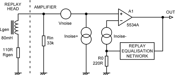
The contributions to the noise at the inputs of A1 are:
- The Johnson noise of the DC resistance of the replay head Rgen.
- The Johnson noise of the 33 kΩ head load resistor Rin. Some of the Johnson noise generated by Rin is shunted away from the amplifier input by the tape head, the amount shunted away decreasing with frequency as the head inductance Lgen increases in impedance. Here the fraction of Rin noise reaching the amplifier rises from 0.003 to 0.21 as frequency increases from 36 Hz to 17.4 kHz.
- The opamp voltage noise Vnoise. This contribution is unaffected by other components.
- The noise voltage generated by Inoise+ flowing through the parallel combination of the replay head impedance and Rin. This impedance increases with frequency due to Lgen. Here it increases from 111 Ω at 36 Hz to 6914 Ω at 17.4 kHz; the increase at the high-frequency end is limited by the shunting effect of Rin. This increase in impedance makes Inoise+ significant and so has an important effect on the noise behaviour. For the lowest noise, you must design for a higher impedance than you might think.
- The Johnson noise of R0. For the values shown, and with A1 assumed to be 5534A, ignoring the Johnson noise of R0 improves the calculated noise performance by only 0.35 dB. The other resistors in the RIAA feedback network are ignored, as R0 has a much lower value and so shunts their contribution to ground, but the replay equalisation frequency response must of course be modelled. More details of the very limited effect that R0 has on the noise performance of amplifiers are given in Chapter 9.
- The noise voltage generated by Inoise- flowing through R0. For normal values of R0, say up to 1000 Ω, this contribution is negligible, affecting the total noise output by less than 0.01 dB.
Using my TAPENOISE mathematical model on Figure 11.3 without replay equalisation gives Table 11.8. Values of Lgen= 100 mH and Rgen= 250 Ω were used to correspond with the heads used for measurements in the next section.
| Coil Lgen= 100 mH | Coil Rgen= 250R | Amp gain | Calc’d Noise out | Meas’d Noise out | Excess noise | |
|---|---|---|---|---|---|---|
| Device | EIN dBu | Noise figure dB | dB | dBu | dBu | dB |
| Noiseless amp | –121.93 | 0.00 | 29.9 | –92.03 | ||
| AD8656 | –120.42 | 2.25 | 29.9 | –90.52 | ||
| BC327 100uA | –120.35 | 2.32 | 29.9 | –90.45 | –86.8 | 5.23 |
| 2SB737 70uA | –119.85 | 2.82 | 29.9 | –89.95 | ||
| OPA828 | –119.11 | 3.56 | 29.9 | –89.21 | ||
| OPA2156 | –119.11 | 3.56 | 29.9 | –89.21 | ||
| 5534A | –118.56 | 4.11 | 29.9 | –88.66 | –86.2 | 3.01 |
| OPA1622 | –116.70 | 5.97 | 29.9 | –86.80 | ||
| 5532A | –116.05 | 6.62 | 29.9 | –86.15 | –85.8 | 2.86 |
| OPA2134 | –115.25 | 7.42 | 29.9 | –85.35 | –84.2 | 1.15 |
| LM4562 | –112.40 | 10.27 | 29.9 | –82.50 | –83.3 | –0.8 |
| TL072 | –109.03 | 13.64 | 29.9 | –79.13 | –78.8 | 0.33 |
| LM741 | –107.90 | 14.77 | 29.9 | –78.00 |
If you compare the table with the similar tables for moving-magnet cartridges (Chapter 9) and guitar pickup (Chapter 12), you will see that the order of merit for the various devices is quite different. This is because the tape head inductance is much lower, and so the effect of device current noise is also much less.
The OPA2134 gave good results with a guitar pickup, but here its relatively high voltage noise drops it down the table with a noise figure (NF) of 7.4 dB. Using an inexpensive 5534A reduces the noise figure 4.1 dB; to improve on that you’ll have to either shell out for some rather expensive new opamps or use a hybrid discrete/opamp amplifier. The much-lamented 2SB737 transistor gets the noise figure down to a rather impressive 2.8 dB, but its 2 Ω Rb is of no help here given the 250 Ω coil resistance of the head, and it is beaten by a BC327 (beta assumed to be 500) running at an Ic of 100uA. Its high beta reduces current noise and drops the NF to 2.3 dB; clearly Studer knew what they were about. The AD8656 wins with NF = 2.2 dB, but its high cost means that a BC327/5532 hybrid solution is very nearly as good and much cheaper.
Replay Noise: Measurements
As related in Chapter 12 on guitar electronics, measuring the noise performance of an amplifier whose input is loaded with a transducer sensitive to magnetic fields can be very difficult. The test amplifier used had a flat frequency response was similar to Figure 11.3 but without equalisation. The replay head used had an inductance of 100 mH, measured by using it in a parallel resonance circuit with a 100 nF capacitor. The resistance was measured as 250 Ω using a digital ohmmeter; if you do this, make sure to demagnetise the head before using it with tape.
The feedback network consisted of R3 = 10 kΩ and R0 = 330 Ω with C3 and R2 omitted, giving a flat gain of +30 dB. (OK, 29.9 dB to be more precise.) Some of the measured results are shown in the rightmost column of Table 11.8 for comparison with the calculated figures. The agreement is good for the TL072 but gets worse as the noise level decreases. This is not due to hum, as the measured noise was in no case significantly affected by switching in a 400 Hz filter, and further investigation is required. The amplifier and head were completely electrically shielded and connected by long leads to test gear approximately 2 metres away to avoid hum from mains transformers.
The BC327 measurement was obtained using a hybrid amplifier closely resembling Figure 11.4. Interestingly, both TL072 and 5532 worked fine for A1, with no measurable difference in noise performance.
You may be wondering how the LM4562 manages an excess noise of -0.8 dB. The answer is that the inputs to the noise calculations are the typical specs for voltage and current noise densities. Clearly I got a good one there.
I measured five samples of each device I had to hand to check out the part-to-part variations; the results are in Table 11.9. All results except for the 5532 are admirably consistent; the 5532s were by various manufacturers including Fairchild, Philips, Texas, and Signetics.
| dBu | dBu | dBu | dBu | dBu | ||
|---|---|---|---|---|---|---|
| Manufacturer | Sample | #1 | #2 | #3 | #4 | #5 |
| Texas | 5534A | –86.2 | –86.2 | –86.4 | –86.5 | –86.4 |
| Various | 5532A | –86.4 | –86.6 | –85.8 | –85.3 | –85.8 |
| Burr–Brown | OPA2134 | –84.1 | –84.2 | –84.2 | –84.3 | –84.2 |
| National | LM4562 | –83.3 | –82.8 | –82.9 | –83.3 | –83.7 |
| Texas | TL072 | –78.8 | –78.9 | –79.1 | –78.9 | –80.7 |
Load Synthesis
The noise performance of an MM phono preamplifier can be improved by 0.8 to 2.9 dB (depending on the noise performance of the basic amplifier) by means of load synthesis; see Chapter 9. This also applies to tape replay preamplifiers and even guitar pickup preamplifiers, because both have the same situation of a large inductance that must be loaded with a high resistance to avoid LF roll-off. The idea is that a high-value resistor can be emulated by a very high-value resistor (which has lower current noise, which is what counts here) if the end that would normally be grounded is driven with an inverted signal, so it appears to be a lower value than it is.
The application of load synthesis to tape replay amplifiers is considered in [14], where its use with a cassette tape head loaded with a 36 kΩ resistor reduced the electronic noise by 5.9 dB (IEC weighted), which is notably better than the phono cartridge case. Nevertheless, I am not aware it has ever been used in a commercial tape machine.
Noise Reduction Systems
It was clear that the basic noise performance of the Compact Cassette was too poor for anything resembling hi-fi, and in 1968, the Dolby-B system was unveiled. [15] (Dolby-A was a much more complex system for professional open-reel use, introduced in 1966.) Dolby-B was a compander system –the dynamic range on tape was reduced by boosting low-level HF content when recording and cutting it on replay, giving a noise reduction of up to 10 dB; this was enough to make cassettes acceptable. There were several other compander noise-reduction systems, such as dbx [16], Telefunken’s High Com [17], and Nakamichi’s High Com II [18], but none were anything like as successful as Dolby-B.
The market acceptance of Dolby-B stemmed from two factors; First, the companding was done by processing low-level signals, with the high levels going through untouched, so artefacts would be less noticeable. Even so, a significant challenge was the need for an acceptably linear variable-gain element, in this case the JFET; VCAs were being introduced but were far too expensive for consumer gear. The Dolby system would probably have never emerged without the invention of the JFET. Since the signal was only processed when it was at low levels, the non-linearity of the JFET was less important than it would have been otherwise. JFETs show considerable variation in their characteristics, and it was necessary to select them into batches and provide at least two adjustments by means of preset resistors.
Second, if you played a Dolby-B encoded tape without a decoder, it sounded brighter in the treble but was generally acceptable to listen to; given the variations in replay head azimuth about it often sounded better. I always used to play back Dolby-B cassettes without decoding in my car stereo, as the level-dependent HF boost helps in a noisy environment.
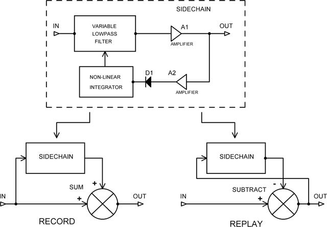
If a companding system is to operate without audible artefacts, the decoding process must be the exact inverse of the encoding process. It would be extremely hard to do this if the two processes were accomplished by different circuitry. An important feature of the Dolby system is that the encoding and decoding were performed by the same circuitry (or different instances of the same circuitry) so that only component tolerances could cause trouble. The heart of the Dolby-B system as shown in Figure 11.6 is the sidechain, which is an HF-only compressor. As the signal level increases, the cutoff frequency of the low-pass filter is reduced so that in Record mode, a decreasing amount of HF is added into the straight-through signal. In replay the sidechain is reconnected so that the output signal is low-pass filtered and then subtracted from the straight-through path, reducing the HF gain and so improving the noise performance.
Dolby-C [19] was a more ambitious consumer companding system introduced in 1980, and basically consisted of two Dolby-B characteristics, giving a noise reduction of about 15 dB (A-weighted). It does not give acceptable results without decoding. It arrived too late to have a major impact on consumer equipment, but found its niche in semi-pro multi-track tape machines such as the Fostex R8, which gave 8-tracks on ¼-inch tape running at 15 ips. My R8 was the centre-piece of my 8-track recording studio, along with the first prototype of the Soundcraft Delta mixer. I still have both.
Bang and Olufsen came up with a technique they called “Auto-Dolby”, which could detect if Dolby-B or Dolby-C was in use and select the correct decoding. You could have different Dolbys on the same tape. However, this only worked if the tape had been recorded on an Auto-Dolby machine in the first place, because subsonic tones were added to the signal to indicate which Dolby was in use. This doesn’t sound particularly useful, and not everyone (myself included) is happy with subsonic tones being added to their audio. The idea appears to have sunk without trace, and rightly so.
Dolby-SR (SR stands for spectral recording) was Dolby’s second professional noise reduction system, aimed at multi-track machines. It gave up to 25 dB of noise reduction at HF. [20] It was very complex, with multiple bands of companding, and never appeared in the consumer market.
Dolby-S was intended to be an advance on Dolby-C for consumer products. It was introduced in 1989, and Dolby claimed most people could not tell the difference between a CD and a Dolby-S cassette. Dolby-S is partly a development of Dolby-C and partly a simplified version of Dolby-SR; it uses one fixed LF band below 200 Hz and two bands working from 400 Hz upwards. The latter are divided into high- and low-level stages, with two 12 dB companders giving 24dB noise reduction at HF when both are fully active. It gives 10 dB of noise reduction at LF. The timing was bad, and it has so far seen little use; however, if we really are going to have a large-scale cassette revival, its day may now have come.
Dolby HX-Pro
A completely different approach to noise reduction was the Dolby HX-Pro variable-bias system [21], where HX stands for headroom extension. HX alone represents the feedforward system developed by Ken Gundry at Dolby [22] and HX-Pro a superior feedback system invented later by Bang and Olufsen in 1980 [23], and licensed to Dolby. When a recording is made with a lot of HF content, it effectively adds to the bias signal and limits the HF levels that can be recorded. HX-Pro reduces the bias level in the presence of high-amplitude HF audio, allowing recording at a higher level for the same distortion and relatively reducing noise. On cassette tape, the improvement is from 7 to 10 dB at 15 kHz. [24]
Figure 11.7 shows the basic principle. The record amplifier has a current-source output (indicated by the two-circle symbol), so it can drive a constant current into the inductive record head at all frequencies. The usual LC bias trap to keep bias out of the record amplifier is shown. The voltage across the head, the sum of the audio and bias signals, is sensed by a high-impedance amplifier (to avoid upsetting the drive/head operation) and then integrated to provide a representation of the current through the head. This is then high-pass filtered, so the feedback loop only works at HF and applied to a rectifier then an error amplifier which compares the total bias level detected with a desired reference level. This creates a correction signal to drive a VCA which controls the amount of bias applied to the head. The feedback operation means that the system works automatically with different signal levels and music spectra. It is only necessary to set the reference to the right bias level for the type of tape being used.
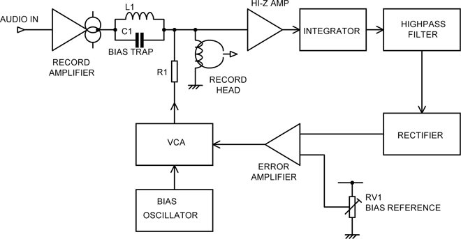
Figure 11.7 Block diagram of Dolby HX-Pro headroom extension system.
HX-Pro only operates when recording, so no decoder is required. It has always struck me as one of the cleverest ideas applied to tape technology. It received wide acceptance, as it did not manipulate the audio, and most HX-Pro machines have it permanently enabled, though some have it as switchable on/off. As an example, the Revox C287 open-reel 8-track machine had HX-Pro but, interestingly, no companding noise reduction.
Two separate HX-Pro circuits are required for stereo recording, as the audio HF content will not be the same in both channels. Only one bias oscillator is used, both for economy and to prevent beat notes. In cassette decks, the complete HX-Pro function was usually implemented by an IC called the uPC1297CA; an example is the Sony TC-D707 (1992). The uPC1297CA was a stereo HX-Pro controller; each channel had a push-pull output to drive a step-up transformer that was connected to the record head.
References
[1] The Guardian www.theguardian.com/music/2019/feb/23/cassette-tape-music-revival-retro-chic-rewind Accessed Sept 2019
[2] The Scotsman www.scotsman.com/arts-and-culture/entertainment/forget-vinyl-it-s-time-for-the-8-track-revival-1-4913166 Accessed Sept 2019
[3] Wikipedia https://en.wikipedia.org/wiki/The_Men_That_Will_Not_Be_Blamed_for_Nothing Accessed Aug 2019
[4] Wikipedia https://en.wikipedia.org/wiki/Elcaset Accessed Aug 2019
[5] Self, Douglas Electronics for Vinyl. Focal Press, 2018
[6] Wikipedia https://en.wikipedia.org/wiki/Audio_tape_specifications Accessed Aug 2019
[7] Wikipedia https://en.wikipedia.org/wiki/Cassette_tape Accessed Aug 2019
[8] Wikipedia https://en.wikipedia.org/wiki/Microcassette Accessed Aug 2019
[9] Carlson & Carpenter “Radio Telegraph System” US patent 1-640-881 (filed Mar 1921; issued Apr 1927)
[10] Engel, F. www.richardhess.com/tape/history/Engel_Walter_Weber_2006.pdf Accessed Aug 2019
[11] Nortronics www.jrfmagnetics.com/Nortronics_pro/nortronics_silver/Nortronics_silver_catalog.pdfAccessed Aug 2019
[12] Camras, M. Magnetic Recording Handbook. Springer, 1988, pp 204–206
[13] Pspatial Audio http://pspatialaudio.com/tape%20equalisation%20correction.htm Accessed Aug 2019
[14] Hoeffelman & Meys “Improvement of the Noise Characteristics of Amplifiers for Magnetic Transducers” Journal of Audio Engineering Society, Vol. 26, No. 12, Dec 1978, p 935
[15] Wikipedia https://en.wikipedia.org/wiki/Dolby_noise-reduction_system#Dolby_B Accessed Aug 2019
[16] Wikipedia https://en.wikipedia.org/wiki/Dbx_(noise_reduction) Accessed Aug 2019
[17] Wikipedia https://en.wikipedia.org/wiki/High_Com Accessed Aug 2019
[18] Wikipedia https://en.wikipedia.org/wiki/High_Com#High_Com_II Accessed Aug 2019
[19] Wikipedia https://en.wikipedia.org/wiki/Dolby_noise-reduction_system#Dolby_C Accessed Aug 2019
[20] Wikipedia https://en.wikipedia.org/wiki/Dolby_SR Accessed Aug 2019
[21] Wikipedia https://en.wikipedia.org/wiki/Dolby_noise-reduction_system#Dolby_HX/HX-Pro Accessed Aug 2019
[22] Gundry, K. “Headroom Extension For Slow-Speed Magnetic Recording Of Audio” JAES Preprint 1534, 64th Convention New York, Nov 1979
[23] Beoworld www.beoworld.org/article_view.asp?id=145 Accessed Aug 2019
[24] Jensen, J. “Recording with Feedback Controlled Effective Bias” JAES Preprint 1852 (J-5), 70th Convention New York, Oct/Nov 1981