CHAPTER 10

GAUSSIAN INFORMATION

In this chapter we look at linear systems with stochastic disturbances. Imagine, for example, that we want to determine a physical state of a certain object by repeated measurement. Then, the observed measurement results are always composed of the real state and some unknown measurement errors. In many important applications, however, these stochastic disturbances may be assumed to have a normal or Gaussian distribution. Together with accompanying observations, such a system forms what we call a Gaussian information. We are going to discuss in this chapter how inference from Gaussian information can be carried out. This leads to a compact representation of Gaussian information in the form of Gaussian potentials, and it will be shown that these potentials form a valuation algebra. We may therefore apply local computation for the inference process which exploits the structure of the Gaussian information. This chapter is largely based on (Eichenberger, 2009).

Section 10.1 defines an important form of Gaussian information that is used for assumption-based reasoning. This results in a particular stochastic structure, called precise Gaussian hint, which is closely related to the Gaussian potentials of Instance 1.6. In fact it provides meaning to these potentials and shows that combination and projection of Gaussian potentials reflect natural operations on the original Gaussian information. This gives sense to the valuation algebra of Gaussian potentials that was introduced in Instance 1.6 on a purely algebraic level. Section 10.2 starts with an illustrative example to motivate a necessary generalization of the concept of Gaussian information and also indicates how inference can be adapted to this more general form. Then, Section 10.3 rigorously carries through the sketched approach, which finally results in an important extension of the valuation algebra of Gaussian potentials. Section 10.2 will also be developed in another direction in Section 10.6. Here, we show that the extended valuation algebra of Gaussian potentials serves to compute Gaussian networks. Finally, Section 10.5 applies the results of this chapter to the important problems of filtering, smoothing and prediction in Gaussian time-discrete dynamic systems.

10.1 GAUSSIAN SYSTEMS AND POTENTIALS

In this section, we consider models that explain how certain parameters generate certain output values or observations. In a simple but still very important case, we may assume that they do this in a linear manner, which means that the output values are linear combinations of the parameters. Often, there are additional disturbance terms that also influence the output. Let us call the parameters x1, …, xn, the observed output values z1, …, zm and let the term which influences observation zi be ωi. The following model describes how the parameters generate the output values

where j = 1, …, m. This is often called a linear functional model. Then, the problem considered in this section is the following: Given this functional model and m observations z1, …, zm, try to determine the unknown values of the parameters x1, …, xm. Since the parameters are unknown, we replace them by variables X1, …, Xm and obtain for j = 1, …, m the system of linear equations

(10.1)

This system rarely has a unique solution for the unknown variables, and it is often assumed that the system is overdetermined, i.e. the number of equations exceeds the number of unknowns, m ≤ n. The method of least squares, presented in Section 9.2.5, provides a popular approach to this problem. It determines the unknowns x1, …, xn by minimizing the sum of squares

We propose a different approach from least squares that yields more information about the unknowns, but at the price of an additional assumption: we assume that the disturbances ωj have a Gaussian distribution with known parameters. For that purpose, it is convenient to change into matrix notation. Let A be the matrix with elements aj,i for i = 1, …, n and j = 1, …, m. X is the vector with components Xi and ω and z are the vectors with components ωj and zj respectively. System (10.1) can then be written as

(10.2)

The vector of disturbances ω is assumed to have a Gaussian distribution as in equation (1.20) with the zero vector 0 as mean and an m × m concentration matrix K. We further assume an overdetermined system where m ≤ n and also that matrix A has full column rank n. This setting is called a linear Gaussian system whereas more general systems are considered in Section 10.3. The following example of a linear Gaussian system is taken from (Pearl, 1988), see also (Kohlas & Monney, 2008; Eichenberger, 2009).

Example 10.1 This example considers the causal model of Figure 10.1 for estimating the wholesale price of a car. There are observations of quantities that influence the wholesale price (i.e. production costs and marketing costs) and quantities that are influenced by the wholesale price (i.e. the selling prices of dealers). Besides, each observation has an associated Gaussian random term that simulates the variation of estimations and profits. We are interested in determining the wholesale price of a car given the final selling prices of dealers and the estimated costs for production and marketing. Let W denote the wholesale price of the car, U1 the production costs and U2 the marketing costs. The manufacturer’s profit U3 is influenced by a certain profit variation ω3. We thus have

The selling prices Y1 and Y2 of two dealers are composed of the wholesale price and the mean profits Z1 and Z2 of each dealer. They are subject to variations ω1 and ω2:

The manufacturer’s production costs U1 are estimated by two independent experts. Both estimates I1 and I2 are affected by estimation errors v1 and v2:

The marketing costs U2 are also estimated by two independent marketing experts. Again, both estimates J1 and J2 are affected by errors λ1 and λ2:

We bring this system into the standard form:

This is an overdetermined system with m = 7 and n = 3. The corresponding matrix A has full column rank.

The idea of assumption-based reasoning is the following; although ω is unknown in equation (10.2), we may tentatively assume a value for it and see what can be inferred about the unknown parameter x under this assumption. First we note this system only has a solution if the vector z - ω is in the linear space spanned by the column vectors of A. The crucial observation of assumption-based reasoning is that all ω which do not satisfy this condition are excluded by the observation of z, since z has been generated by some parameter vector x according to the functional model (10.2). Thus, admissible disturbances ω are only those vectors for which (10.2) has a solution. In other words, the observation z defines an event

in the space of disturbances and we have to condition the distribution of ω on this event. The set vz is clearly an affine subspace of m. In order to compute this conditional distribution, we apply a linear transformation to the original system (10.2) which does not change its solutions. Since the rank of matrix A equals n, there must be n linearly independent rows in A. If necessary, we renumber the equations and can therefore assume that the first n rows are linearly independent. They form a submatrix A1 of A, and A2 denotes the submatrix formed by the remaining m - n rows. We then define the m × m matrix

where Im-n is the (m - n) × (m - n) identity matrix. Clearly, B has full rank m and has therefore the inverse

Let us now consider the transformed system TAX + Tω = Tz. Since the matrix T is regular this system has the same solutions as the original. This system can be written as

(10.3)

where

and z1, ω1 and z2, ω2 are the subvectors of the first n and the remaining m - n components of z and ω respectively. The advantage of the transformed system (10.3) is that the solution is given explicitly as a function of , whereas has a constant value. In this situation, the conditional density of given can be determined by classical results of Gaussian distributions (see appendix to this chapter). First, we note that the transformed disturbance vector with the components and has still a Gaussian density with mean vector 0 and concentration matrix

The correctness of the first equality will be proved in Appendix J.2. Then, the conditional distribution of given is still Gaussian and has concentration matrix ATKA (see Appendix J.2) and mean vector

Note now that according to (10.3) we have

Since the stochastic term has a Gaussian distribution, the same holds for X. In fact, it has the same concentration matrix ATKA as . Its mean vector is

We thus obtain for the unknown parameter in equation (10.2) a Gaussian density or a Gaussian potential

(10.4)

Assumption-based reasoning therefore infers from an overdetermined linear Gaussian systems a Gaussian potential. How is this result to be interpreted? The unknown parameter vector x is finally not really a random variable. Assumption-based analysis simply infers that for a feasible assumption ω about the random distributions, the unknown parameter vector would take the value . But this expression has a Gaussian density with parameters as specified in the potential above. So, a hypothesis about x, like x ≤ 0 for instance, is satisfied for all feasible assumptions ω satisfying , and the probability that the assumptions satisfy this condition can be obtained from the Gaussian density above. This is the probability that the hypothesis can be derived from the model. The Gaussian density determined by the Gaussian potential is also called a fiducial distribution. The concept of fiducial probability goes back to the statistician Fisher (Fisher, 1950; Fisher, 1935). For its present interpretation in relation to assumption-based reasoning we refer to (Kohlas & Monney, 2008; Kohlas & Monney, 1995).

Example 10.2 We first execute a diagnostic estimation/or the linear Gaussian system of Example 10.1. The term diagnostic means that observations are given with respect to the variables that are influenced by the wholesale price. These are the selling prices and the mean profits of both dealers, and inference is performed on the disturbance vector ω = [ω1 ω2]. We thus consider the first two equations of the system:

If σωii denotes the variance of the disturbance ωi associated to Yi we have

With respect to equation (10.4) we compute

and

Finally, we obtain the following Gaussian potential for the wholesale price W given Y1, Y1, Z1 and Z2 in the above system:

Example 10.3 Let us next execute a predictive estimation for the Gaussian system of Example 10.1. The term predictive means that observations are given with respect to the variables that influence the wholesale price. These are the production costs U1 and the marketing costs U2 which are estimated by two experts, and the industry profit U3 for which we have one estimation. We thus consider the remaining subsystem:

Observe that the last equation W = U1 + U2 + U3 + ω3 defines the wholesale price as a linear combination of the production costs, marketing costs and the industry profit. We may therefore conclude that the same holds for the Gaussian potential of the wholesale price given the estimations for the production costs, marketing costs and the industry profit. We have

where

and

A similar analysis as in Example 10.2 gives:

and

with

Next, we are going to relate the operations of combination and projection in the valuation algebra of Gaussian potentials from Instance 1.6 to linear Gaussian systems. For this purpose, we fix a set r of variables with subsets s and t. So, let X denote an (s ∪ t)-tuple of variables. We consider the system of linear equations with Gaussian disturbances composed of two subsystems,

Here, we assume that A1 is an m1 × s matrix, A2 an m2 × t matrix and z1, ω1 and z2, ω2 are m1 and m2-vectors respectively. Both matrices are assumed to have full column rank |s| and |t| respectively. Further, we assume that ω1 has a Gaussian density with mean 0 and concentration matrix K1, whereas ω2 has a Gaussian density with mean 0 and concentration matrix K2. Both vectors are stochastically independent. Now, we can either determine the Gaussian potentials of the two systems:

and

or we can determine the Gaussian potential of the combined system

Here, the disturbance vector has the concentration matrix

Remark that the matrix of this combined system has still full column rank |s ∪ t|. The Gaussian potential of the combined system is (μ, K) with

Note that this is exactly the concentration matrix of the combined potential G1 G2 given in equation (1.21). For the mean vector μ of the combined system we have:

Let now μ1 = (A1T K1A1)−1 A1K1z1 and μ2 = (A2TK2A2)−1 A2K2z2 be the mean vectors of the two potentials G1 and G2. We then see that we can rewrite the last expression above as

But this is the mean vector of the combined potential as shown in equation (1.22). Thus, we have shown that

Therefore, combining two linear Gaussian systems results in the Gaussian potential, which is the combination of the Gaussian potentials of the individual systems. This justifies the combination operation which itself is derived from multiplying the associated Gaussian densities. The combination of Gaussian potentials as defined in Instance 1.6 therefore makes much sense.

Example 10.4 Let us now assume that all values in the system of Example 10.1 have been observed. Then, inference can either be made for the complete model, or by combining the two potentials derived from the submodels in Example 10.2. We have

The two components of the combined potential are:

and

Note that since we are dealing with potentials over the same single variable, there is no need for the extensions in the definition of combination. This is an example of solving a rather large system by decomposition and local computation. However, we remark that the theory is not yet general enough since the subsystems for the decompositions do not always have full column rank.

Now, suppose that X is a vector of variables from a subset s r which represents unknown parameters in a linear Gaussian system (10.1). Inference leads to a Gaussian potential (μ, K) = ((ATKωA)−1 ATKωz, (ATKωA)). If t is a subset of s, and we are only interested in the parameters in , it seems intuitively reasonable that for this vector the marginal distribution of the associated Gaussian density is the correct fiducial distribution. This marginal is still a Gaussian density with the corresponding potential . It corresponds to the projection of the Gaussian potential (μ, K) to t as defined in Instance 1.6:

(10.5)

In fact, this can be justified by the elimination of the variables in the system (10.1), but it is convenient to consider for this purpose the equivalent system (10.3). The second part of this system does not contain the variables at all, and in the first part we simply have to extract the variables in the set t to get the system

The distribution of has not changed by this operation. This therefore shows that the fiducial density of is indeed the marginal of the fiducial density of X (for the marginal of a Gaussian density see Appendix J.2).

By these considerations, Gaussian potentials are strongly linked to certain Gaussian systems, and the operations of combination and projection in the valuation algebra of Gaussian potentials are explained by corresponding operations on linear Gaussian systems. The valuation algebra of Gaussian potentials therefore obtains a clear significance through this connection. In particular, Gaussian potentials can be used to solve inference problems for large, sparse systems (10.1), since they can often be decomposed into many much smaller systems. This will be illustrated in the subsequent parts of this chapter. However, it will also become evident that an extension of the valuation algebra of Gaussian potentials will be useful and even necessary for some important problems. We finally refer to Section 9.2.5 where a different interpretation of the same algebra based on the least squares method is given.

10.2 GENERALIZED GAUSSIAN POTENTIALS

The purpose of this section is to show that the valuation algebra of Gaussian potentials is not always sufficient for the solution of linear, functional models by local computation. To do so, we present an important instance of such models named time-discrete, dynamic system with Gaussian disturbances and error terms.

10.1 Gaussian Time-Discrete Dynamic Systems

Let X1, X2, … be state variables where the index refers to the time. The state at time i + 1 is proportional to the state at time i plus a Gaussian disturbance:

The state cannot be observed exactly but only with some measurement error. We denote the observation of the state at time i by zi such that

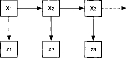
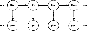
We further assume the disturbance terms ωi and the measurement errors vi to be mutually independent. The ωi are all assumed to have a Gaussian density with mean 0 and variance σw2, whereas the observation errors vi are assumed to have a Gaussian density with mean 0 and variance σv2. Such a system has an illustrative graphical representation which indicates that state Xi+1 is influenced by state Xi and observation zi by state Xi. This is shown in Figure 10.2. It resembles a Bayesian network like the one in Instance 2.1 with the difference that the involved variables are not discrete but continuous. The computational problem is to infer about the states of the system at time i = 1,2, … given the equations above and the measurements zi of the states at different points in time.

Let us now consider a manageable size of this instance where zi for i = 1, 2, 3 is given and the states X1, X2 and X3 are to be determined. Then, the equations above can be rewritten in a format corresponding to the linear Gaussian systems introduced in the previous section:

(10.6)

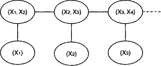
The first equation has been added to indicate an initial condition on state X1. If we consider each individual equation of this system as a piece of information, or as a valuation, then we obtain a covering join tree for the system as shown in Figure 10.3. Each equation of the system is on one of the nodes of the join tree. This constitutes a nice decomposition of the total system. If we could derive a Gaussian potential for each node, we could solve the problem specified above by local computation. However, although each equation represents a linear Gaussian system, it does not satisfy the requirement of full column rank imposed in the previous section. In fact, the single equations do not represent overdetermined systems, but rather underdetermined systems. So, unfortunately, we cannot directly apply the results from the previous section and work with Gaussian potentials. This indicates the need of an extension of the theory of inference in linear Gaussian systems.

In order to introduce the new concepts needed to treat such systems, let us have a closer look at the first two equations of system (10.6):

(10.7)

Its matrix and vector are

The disturbance vector ω = [ω1 ω2] has the concentration matrix

Finally, if X denotes the variable vector with components X1 and X2, the system (10.7) can be represented in the standard form (10.2) of Section 10.1:

This system has full column rank 2 and thus fulfills the requirement of assumption-based reasoning imposed in Section 10.1. We derive for X a Gaussian potential

with

The mean vector of X can be obtained from system (10.7) directly,

(10.8)

or from the results of Section 10.1. The fact that A has an inverse simplifies this way.

We now look at this result from another perspective. If we consider the second equation of system (10.7) in the form X2 = aX1 + ω1, we can read from it the conditional Gaussian distribution of X2 given X1 as a Gaussian density fX2|X1 with mean ax1 and variance σω2. This is the same conditional density as we would get from the Gaussian density of X above by conditioning on X1. Hence, this conditional density of X2 given X1 can also be obtained as the quotient of the density fX of X divided by the marginal density fX1 of X1, which is Gaussian with mean m and variance σω2. If we compute this quotient, we divide two exponential functions, and, neglecting normalization factors, it is sufficient to look at the exponent, which is the difference of the exponent of fX and fX1,

The second term of this expression can be written as

where KX1 = [1/σω2] is the one-element concentration matrix of X1. If we introduce this in the exponent of the conditional Gaussian density above, we obtain

This looks almost like a Gaussian density, except that the concentration matrix KX2|X1 in this exponent is only non-negative definite and no more positive definite, since it has only rank 1. We remark that this concentration matrix is essentially the difference of the concentration matrices of fX and fX1,

This observation leads us to tentatively introduce a generalized Gaussian potential (μ, KX2|X1) where μ is still given by (10.8). It is thought that this potential represents the conditional Gaussian distribution of X2 given X1. This will be tested in a moment.

Remark that from the first equation of (10.7), it follows that X1 has a Gaussian density fX1 with mean m and variance σω2. This is the marginal obtained from the density fX and it is represented by the ordinary Gaussian potential (m, 1/σω2). The vector X then has the Gaussian density fx = fX2|X1. Let us try whether we get this also by formally applying the combination rule to the Gaussian potential for X1 and the generalized potential of X2 given X1. So, let

According to the combination rule for potentials denned in Instance 1.6 we have

This is indeed the concentration matrix of fX. Let us see whether this also works for the mean vector. We first determine

According to the combination rule for potentials defined in Instance 1.6 we have

This is indeed the mean vector of fX It seems that the combination operation for ordinary potentials works formally also with generalized Gaussian potentials.

We shall see later that it is even more convenient to define the generalized Gaussian potentials as (Kμ, K). Indeed, we remark that the generalized Gaussian potential of X2 given X1 can also be determined directly from the second equation of system (10.8) which defines the conditional density. Let A = [a -1] be the matrix of this equation and Kω = [1/σω2] its concentration matrix. We consider the exponent of the exponential function defining the conditional density of X2 given X1:

From this we see that indeed

Further, we obtain

So, indeed, the generalized Gaussian potential is completely determined by the elements of the defining equation only. This approach can be developed in general, and it will be done so in Section 10.3. For the time being, we claim that the same procedure can be applied to the equations associated with the nodes of the join tree in Figure 10.3. We claim, and show later, that the extended Gaussian potentials form again a valuation algebra, extending the algebra of ordinary Gaussian potentials. The Gaussian potential of the total system (10.6) can therefore be obtained by combining the generalized Gaussian potentials. The fiducial densities of the state variables is then obtained by projecting this combination of potentials to each variable. Thus, the inference problem stated at the beginning of this section can be solved by local computation with very simple data rather than by treating system (10.6) as a whole. This example is a simple instance of a general filtering, smoothing and projection problem associated with time-discrete Gaussian dynamic systems. It will be examined in its full generality in Section 10.5. Moreover, can also be seen as an instance of a Gaussian Bayesian network. This perspective will be discussed in Section 10.6.

10.3 GAUSSIAN INFORMATION AND GAUSSIAN POTENTIALS

In this section, we take up the approach sketched in the previous Section in a more systematic and general manner by considering arbitrary underdetermined linear systems with Gaussian disturbances.

10.3.1 Assumption-Based Reasoning

Let us assume a linear system with Gaussian disturbances

(10.9)

which, in contrast to Section 10.1, is underdetermined. Here, X is an n-vector, A an m × n matrix with m ≤ n and z an m-vector. The stochastic m-vector ω has a Gaussian density with mean vector 0 and concentration matrix Kω. Further, we assume for the time being that A has full row rank m. More general cases will be considered later.

We first give a geometric picture of this situation based on the approach of assumption-based reasoning. Note that, under the above assumptions, system (10.9) has a solution for any vector . So, in contrast to the situation in Section 10.1 with overdetermined systems, no ω has to be excluded, and for any the solution space is an affine space + y(ω) in n. Here, is the kernel (see Section 7.2) of the system and y(ω) any particular solution of the system with a fixed ω. It is evident that the different assumptions lead to disjoint, parallel, affine spaces. Therefore, we sometimes call the focal space associated with ω. It is also clear that if ω varies over m, then their focal spaces cover the whole space n. The Gaussian probability distribution of ω induces also an associated Gaussian probability of the focal spaces. Such a structure is also called a hint: Each assumption ω out of a set of possible assumptions determines a set of possible values for

the unknown parameter x, and the assumptions are not all equally likely but have a specified probability distribution. We refer to (Kohlas & Monney, 1995) for a general theory of hints and to (Kohlas & Monney, 2008) for the connection of hints with statistical inference. If B is a regular m × m matrix, then the transformed system BAX + and has the same family of parallel focal spaces as the original system and also the same Gaussian density over the focal spaces. Such hints, which differ from each other only by a regular transformation, are therefore called equivalent. If m = n, we have an important special case: the focal spaces then reduce to single points, i.e. the unique solutions y(ω) = A−1 (z - ω) of the system for a fixed assumption ω. We refer to the system (10.7) and its analysis in the previous Section 10.2 as an example for such a situation. It induces an ordinary Gaussian density with mean vector A−1z and concentration matrix ATKωA. This case is also covered in Section 10.1, and the Gaussian density corresponds to the Gaussian potential (A−1z, ATKω A) associated with the system. This can indeed be verified from (10.4) in Section 10.1: for the concentration matrix we have the same expression. The mean vector in (10.4) can be developed in this particular case as follows:

Hints with one-point focal spaces result from assumption-based reasoning according to Section 10.1 from any overdetermined system.

In the following, we usually assume m strictly smaller than n. We show that in this case Gaussian conditional densities can be associated with linear Gaussian systems (10.9) and thus also with generalized Gaussian potentials as exemplified in the previous section. Since A has full row rank m, there is at least one m × m regular submatrix of A. By renumbering columns we may always assume that the first m columns of A are linearly independent. We decompose A into the regular submatrix A1 composed of the first m columns and the remaining m × (n - m) submatrix A2, that is A = [A1, A2]. Let us further decompose the vector of variables X accordingly into the m-vector X1 and the (n - m)-vector X2. Then, the system (10.9) can be written as

Applying the regular transformation B = A1−1 yields the equivalent system

where and . The stochastic vector still has a Gaussian density with mean 0 and concentration matrix as shown in the appendix of this chapter. Using the transformed system, we can express X1 by X2,

If we fix X2 to some value x2, we can directly read the Gaussian conditional density of X1 given X2 = x2 as a Gaussian density with mean-vector μX1 | x2 and concentration matrix Kx1|x2 obtained as follows:

This conditional Gaussian density of X1 given X2 has the exponent

(10.10)

Next, we are going to associate a generalized Gaussian density to this conditional Gaussian density in a way similar to that of the previous Section 10.2: To do so, we introduce two undetermined vectors μ1 and μ2 which are linked by the relation

This also means that

(10.11)

The vectors μ1 and μ2 are only used temporarily and will disappear in the end. We introduce this expression into the exponent of equation (10.10):

This looks like the exponent of a Gaussian density with concentration matrix

Since this matrix is only non-negative definite, we call it a pseudo-concentration matrix. The conditional Gaussian density above has an undetermined mean vector μ with components μ1 and μ2, but this mean vector disappears if we consider

The last equality follows from (10.11). To sum it up, we have associated a generalized Gaussian potential

(10.12)

with the original linear Gaussian system (10.9). We have done this via a conditional density extracted from the system (10.11). Note that there may be several different conditional Gaussian densities that can be extracted from (10.11), depending on which set of m variables we choose to solve for. But the final generalized conditional Gaussian potential is independent of this choice. It only depends on the Gaussian information expressed by the system (10.9). Let us verify this assertion by considering an m × m regular matrix B and the corresponding transformed system , where . The generalized potential associated with this transformed system has concentration matrix

Similarly, we obtain for the first part of the generalized potential

So, the transformed equivalent system has the same potential as the original system. In other words: equivalent systems have identical generalized Gaussian potentials.

10.3.2 General Gaussian Information

Linear Gaussian information can be represented in a compact form by generalized Gaussian potentials. How are natural operations with linear Gaussian information reflected by Gaussian potentials? Here, we look at the operations of combination. For subsets s and t of some set of indices of variables let X be an (s ∪ T)-vector and consider two pieces of linear Gaussian information, one referring to the group of variables in s

(10.13)

where A1 is an m1 × s matrix and ω1 and z1 are m1-vectors. ω1 has a Gaussian density with mean vector 0 and concentration matrix Kω1. The second piece of linear Gaussian information refers to the set t of variables,

(10.14)

where A2 is an m2 × t matrix and ω2 and z2 are m2-vectors. ω2 has a Gaussian density with mean vector 0 and concentration matrix Kω2. Together, the two systems provide linear Gaussian information for the total vector X,

(10.15)

The (m1 + m2)-vector ω has a Gaussian density with mean vector 0. Since we assume that the vectors ω1 and ω2 are stochastically independent, its concentration matrix is

The (m1 + m2)-vector z is composed of the two vectors z1 and z2. Finally, the (m1 + m2) × (s ∪ t) matrix A is composed of the matrices A1 and A2 as follows:

(10.16)

Now, even if the two matrices A1 and A2 have full row rank, this is no more guaranteed for the matrix A. Therefore, we need to extend our assumption-based analysis to the case of a general linear Gaussian system

(10.17)

before we can return to the combined system above. Here, we assume A to be an m × n matrix of rank k ≤ m, n. The number of equations m may be less than, equal to or greater than the number of variables n. So, the following discussion generalizes both particular cases studied so far. The vectors ω and z have both dimension m, and ω has a Gaussian density with mean 0 and Kω as concentration matrix. As usual, we consider the system to be derived from a functional model where the linear, stochastic function Ax + ω determines the outcome or the observation z. Then, by the usual approach of assumption-based reasoning, we first remark that, given the observation z, only assumptions ω in the set

may have generated the observation z. The set vz is an affine space in the linear space m and in general different from m. These are the admissible assumptions. Then, each admissible assumption determines the set of possible parameters x by

As before, these are parallel affine subspaces of n which cover n completely. It is also possible that the affine spaces are single points. Different admissible assumptions ω have disjoint focal spaces Γ(ω).

Next, we need to determine the conditional density of ω, given that ω must be in the affine space vz. As in Section 10.1, we transform the system (10.17) in a convenient way which allows us to easily derive the conditional density. For this purpose, we select an m × k matrix B1 whose columns form a basis of the column space of matrix A. For example, we could take k linearly independent columns of A, which is always possible since A has rank k. Consequently, the matrix B1 has rank k. Then, there is a k × m matrix such that A = B1 . We complete B1 with an m × (m - k) matrix B2 such that B = [B1 B2] is a regular m × m matrix and define T = B−1. We decompose

such that T1 is a k × m and T2 an (m - k) × m matrix. Then, we see that

since TB = I implies that T2B1 = 0. Now, the matrix TA has rank k because T is regular. This implies that the k × m matrix T1A has full row rank k. The focal spaces for ω can now be described by

and the admissible assumptions by

This corresponds to the transformed system

(10.18)

where and . The transformed vector is composed of the components . It is still Gaussian with mean 0 and concentration matrix

(10.19)

From the system (10.18) it is now easy to determine the conditional Gaussian density of given . According to equation (10.19) it has concentration matrix B1T KωB1 and mean vector (see Appendix J.2)

Finally, we obtain from system (10.18) the following linear Gaussian system

(10.20)

where

(10.21)

This is now a linear Gaussian system with full row rank k. Therefore, we can apply the results from Section 10.3.1 to derive its generalized potential.

We now argue that this is also the generalized Gaussian potential associated with the original system. In fact, the selection of the basis B1 was arbitrary, and the resulting system depends on this choice, but the associated generalized Gaussian potential does not, as we show next. A linear Gaussian system like (10.17) is fully determined by the three elements A, z and Kω. Therefore, we represent it by the triplet (A, z, Kω) and define the mapping

The image of this mapping looks like a generalized Gaussian potential. In fact, it is one, but it remains to verify that the matrix AT Kω A is non-negative definite. This however is a consequence of the following theorem:

Theorem 10.1 Let l = (A, z, Kω) describe a linear Gaussian system (10.17) with an m × n matrix A of rank k, and

a system with full row rank derived from it as in (10.20) and (10.21). Then, e(l) = e(h).

Proof: We define

It follows that . But then, if B is the matrix used in transforming the system (A, z, Kω) and T = B−1

Further,

So, indeed the generalized Gaussian potential of h equals e(l).

Since e(h) is indeed a generalized Gaussian potential, it follows that e(l) is one too. Thus, by the mapping e(l), we associate a uniquely determined generalized Gaussian potential to each linear Gaussian information of the form (10.17) without any restriction on the rank of the system. We may say that two linear Gaussian systems l and l’ are equivalent if they induce equivalent systems h and h’ with full row rank. Since we have seen that equivalent systems h and h’ generate the same generalized Gaussian potential, this also holds for equivalent Gaussian systems.

10.3.3 Combination of Gaussian Information

We are now able to compute the generalized Gaussian potential (v, K) of the combined system (10.15) with the combined matrix (10.16). Note first that the generalized Gaussian potential (v1, K1) corresponding to the first subsystem (10.13) is given by

(10.22)

and

(10.23)

For the second subsystem (10.14), we have similar results, essentially replacing A1 by A2, Kω1 by Kω2 and z1 by z2. Now, the second part of the potential (v, K) of the combined system (10.15) is given by

The last equality can be concluded from equation (10.22).

Next, we compute the first part of the potential (v, K) of the combined system

This shows how generalized Gaussian potentials can be combined in order to reflect the combination of the linear Gaussian information. Namely, if the potential (v1, K1) has domain s and (v2, K2) has domain t,

10.3.4 Projection of Gaussian information

After the operation of combination, we examine the operation of information extraction or projection. We start with a linear Gaussian system

(10.24)

where X is an s-vector of variables, A an m × s matrix, representing m equations over the variables in s, z an m-vector and ω a stochastic m-vector having Gaussian density with mean vector 0 and concentration matrix Kω. We want to extract from this Gaussian information the part of information relating to the variables X↓t for some subset t s. To this end, we decompose the linear system according to the variables X↓s-t and X↓t,

(10.25)

Here, A1 is the m × (s - t) matrix containing the columns of A which correspond to the variables in s - t, and A2 the m × t matrix containing the columns of A which correspond to the variables in t. Extracting the information bearing on the variables in t means to eliminate the variables in s - t from the linear system above. This operation has already been examined in Chapter 9. But here, we additionally look at the stochastic component ω in the system. To simplify the discussion, we first assume that A1 has full column rank |s - t| = k. This implies that there are k linearly independent rows in the matrix A1. By renumbering rows, we may assume that the first k rows are linearly independent such that the matrix A1 decomposes into a regular k × k submatrix A1,1 composed of the first k rows and the (m - k) × k submatrix A2,1 containing the remaining rows. If we decompose system (10.25) accordingly into the system of the first k equations and the m - k equations, we obtain

Here, A1,2 is a k × (s t) matrix and A2,2 an (m - k) × (s t) matrix. The vectors ω1 and z1 have dimensions k, whereas ω2 and z2 have dimension m - k. Since A1,1 is regular, we can solve the first part for X↓s-t and replace these variables in the second part of the system,

This is a new linear Gaussian system

(10.26)

with

(10.27)

and

We note that in the second part of the linear system (10.26) the variables in s - t are eliminated. Therefore, this part of the system represents the part of the original Gaussian information (10.24) bearing on the variables in t, that is

(10.28)

Here, the matrix corresponds to the right lower element of the matrix . This linear Gaussian information can be represented by the generalized Gaussian potential , where

(10.29)

In order to fully determine this potential, it only remains to compute . For this purpose, note that with the matrix

The inverse of this matrix is

From this we obtain the concentration matrix of ,

(10.30)

Here, A1 is the matrix of X↓s-t in the system (10.25), whereas

denotes the lower row in the decomposition of Kω. We finally obtain the concentration matrix of the marginal density of , and it is shown in Appendix J.2 that this also corresponds to the concentration matrix of ,

(10.31)

We have completely determined the information for X↓t, once as extracted from the original system and then as the associated generalized Gaussian potential. It is very important to remark that these results do not depend on the particular choice of the regular submatrix A1,1 of A1, which is used in the variable elimination, since only the matrix A1 appears in the generalized Gaussian potential.

We want to see whether and how this potential relative to the extracted information can directly be obtained from the generalized Gaussian potential (v, C) of the original system (10.24). As we have shown, equivalent systems have identical potentials. So, instead of computing the potential of system (10.24), we can as well compute the potential of the transformed system (10.26) with the matrix as defined in (10.27). For the pseudo-concentration matrix we have

The matrix denotes the left-hand column of the matrix in (10.27), whereas denotes the right-hand column. Here, C is decomposed with respect to s - t and t. The blocks of C are as follows, if the internal structure of matrix in (10.27) is used:

The last term equals the left upper element of in (10.30). We thus obtain

If and denote the submatrices of corresponding to the decomposition with respect to s - t and t, we obtain for the lower right element of C using (10.30)

Next, we compute the lower left element of C:

By the symmetry of the matrix C it finally follows that

These elements are sufficient to establish the relation between the concentration matrix C in the potential of the original system (10.24) and the concentration matrix in the potential of the reduced system (10.28). In fact, we conjecture that the same projection rule applies as for ordinary Gaussian potentials (10.5) in its transformed form (Cμ, C), i.e.

see Appendix J.2. This can easily be verified by using the above results for the submatrices Ci,j to obtain

see equation (10.29). Similarly, we examine the first part v of the potential,

We find for its two components

We next want to apply the projection rule for ordinary Gaussian potentials from equation (10.5) to the first part of the potential. This requires first transforming the rule to the new form of the potential. From v = Cμ we derive

From this we obtain

So, the conjecture is

In fact,

see equation (10.29). Putting things together, we conclude that generalized and ordinary Gaussian potentials essentially share the same projection rule

This, however, does not yet cover the general case, since we assumed for the extraction of information that the matrix A1 has full column rank, i.e. that all columns of A1 are linearly independent, which is not always the case. Fortunately, it is now no more difficult to treat the general case. So, we return to the original system (10.24) together with its decomposition (10.25) according to the variables in s - t and t. But this time we allow that the rank k of A1 may be less than the number of columns, k < |s - t|. Then, there are k linearly independent columns in A1 and we again assume that these are the k first columns. Denote the matrix formed by these k linearly independent columns by A1’ and the matrix formed by the remaining |s - t| - k columns by A1“. The columns in the second matrix can be expressed as linear combinations of the first k columns. This means that there is a k × (m - k) matrix such that

Within the matrix A1’ of these first k columns there is a regular k × k submatrix. Now, if we decompose the matrix A of the system (10.24) according to k, |s - t| - k and |t| columns and the rows according to the first k and the remaining m - k rows, we have

The system (10.24) then decomposes accordingly, if x denotes the set of variables associated with the first k columns of A1 and y the set of variables associated with its remaining columns such that x ∪ y = s - t, we have

As before, the first part of this system can be solved for X↓x + λX↓y which gives

We observe that ω is transformed into just as before and consequently, still has the concentration matrix as computed in (10.30). It follows from equation (10.31) that the same holds for . As above we define the matrix

where the submatrices (left-hand column), and (right upper and lower submatrices) are still the same. As a consequence, the generalized Gaussian potential of the projected system

does not change and equation (10.29) still holds. In contrast, the potential of the original system changes somewhat. If we define

we obtain

Writing Ci,j for the submatrices above and i, j = 1,2,3, we remark that C1,1 is the old C1,1 computed above, C3,3 is the old C2,2, C3,1 and C1,3 are the old C2,1 and C1,2. It only remains to compute the new C2,2 C2,1, C3,2 and the symmetric C1,2 and C2,3. From the matrix above one easily obtains

The remaining matrices C1,2 and C2,3 are the transposes of C2,1 and C3,2. As before, it follows from these remarks that

More generally, it is now easy to verify that

and also that

This clarifies the general situation concerning extraction of information or projection. The following theorem summarizes this important result:

Theorem 10.2 Consider the linear Gaussian system l: AX + ω = z for the set s of variables and the system for t s obtained by eliminating the variables in s - t. If (v, C) = e(l) is the generalized Gaussian potential for the system l, then there is a subset x y = s - t such that C↓x is regular of rank rank(C↓x) = rank(C↓y). For each such subset x,

There may be several subsets x s - t for which the statement of the theorem holds, and for each such subset the generalized potential e(l↓t) is the same. In practice, this projected potential will be computed from the original potential (v, C) by successive variable elimination. Gaussian potentials summarize the information contained in a linear Gaussian system. In the following section, we show that these potentials form a valuation algebra that later enables the application of local computation for the efficient solution of large, linear Gaussian systems. Illustrations are given in Section 10.5 and 10.6.

10.4 VALUATION ALGEBRA OF GAUSSIAN POTENTIALS

In the previous section, we defined combination of generalized Gaussian potentials, representing union of the underlying linear Gaussian systems, and projection of generalized Gaussian potentials, representing extraction of information in the corresponding linear Gaussian system. In this section, we show that the generalized Gaussian potentials form a valuation algebra under these operations and that the valuation algebra of ordinary Gaussian potentials introduced in Instance 1.6 essentially is a subalgebra of this valuation algebra. For this purpose, we show that hints form a valuation algebra isomorphic to the algebra of generalized Gaussian potentials.

To start, we formally define the algebra under consideration. Let r be a set of variables and D the subset lattice of r. For any non-empty subset s r we consider pairs (v, C) where C is a symmetric, non-negative definite s × s matrix and v an s-vector in the column space of C. Denote by Φs the set of all such pairs. For the empty set we define . Finally, let

to be the set of all pairs (v, C) with domain subset of r. The elements of Φ are called generalized Gaussian potentials, or shortly, potentials. Note that ordinary Gaussian potentials in the form (Kμ, K) also belong to Φ. Within Φ we define the operations of a valuation algebra as follows:

Instead of directly verifying the valuation algebra axioms for these operations, it is easier to examine a corresponding algebra of hints. Indeed, we know that potentials faithfully represent the associated operations with linear Gaussian systems, in particular with Gaussian hints. It turns out to be easier to verify the axioms of a valuation algebra with hints rather than with potentials. We remember however that operations with hints are not uniquely defined. For example, depending on how the variables in s - t are eliminated in a hint h: AX + ω = z on variables s, the reduced systems are different, but equivalent. Therefore, rather than considering individual hints h, we must look at classes of equivalent hints [h]. So, as with potentials, we define Ψs to be the family of all classes [h] where h are hints relating to the subset s r of variables and

As above, we represent hints h by triplets (A, z, K) where A is an m × s matrix with full row rank, hence m ≤ |s|, z is an m-vector and K a symmetric, positive definite s × s matrix. In order to define the basic operations of labeling, combination and projection with hints we denote the operation of the union of two linear systems l1 = (A1, z1, K1) and l2 = (A2, z2, K2) on variables s and t respectively by

Similarly, for a system l = (A1, z1, K1) on variables in s and t s, let

denote a system like (10.28) were the variables in s - t have been eliminated. Finally, if l is a linear Gaussian system, then let h(l) denote the equivalence class of hints derived from l. We are now able to define the basic operations in Ψ:

These operation are all well-defined, since equivalent systems have equivalent unions and projections. The very technical proof of the following theorem can be found in Appendix J.1.

Theorem 10.3 The algebra of hints (Φ, D) with labeling, combination and projection satisfies the axioms of a valuation algebra.

We show that the algebra of generalized Gaussian potentials (Φ, D), which consists of the potentials associated to the hints , also forms a valuation algebra. We first recall that the mapping e: Ψ → Φ, defined by e([h]) = e(h), respects labeling, combination and projection

This has been shown in Section 10.3. Further, we claim that the mapping is onto. In fact, let (v, C) be an element of Φ. C is therefore a symmetric, non-negative definite s × s matrix and v an s-vector in the column space (C) of C. For any symmetric non-negative definite s × s matrix C of rank k ≤ |s|, there exists a k × s matrix A of rank k such that C = AT A. This is a result from (Harville, 1997). The columns of C span the same linear space as AT and therefore, there is a k-vector z such that

Consequently, h = (A, z, Ik) is a hint on s such that

The fact that (Ψ, D) is a valuation algebra then implies that (Φ, D) is a valuation algebra, too, and that both algebras are isomorphic.

We have seen in Section 10.1 that Gaussian hints h = (A, z, K), where A has full column rank, are represented by ordinary Gaussian potentials

that in turn determine Gaussian densities. Such a potential can also be one-to-one transformed into a generalized Gaussian potential (ATKz, ATKA), and combination as well as projection of ordinary Gaussian potentials correspond to the operations on generalized Gaussian potentials. Thus, the original valuation algebra of ordinary Gaussian potentials can be embedded into the valuation algebra of generalized Gaussian potentials and can therefore be considered as a subalgebra of the latter. These insights are summarized in the following theorem:

Theorem 10.4 Both algebras of hints (Ψ, D) and generalized Gaussian potentials (Ψ, D) are valuation algebras and e: Ψ Φ is an isomorphism between them. The valuation algebra of ordinary Gaussian potentials is embedded into (Φ, D).

Consequently, we may perform all computations with hints also with generalized Gaussian potentials. This will be exploited in the remaining sections of this chapter.

10.5 AN APPLICATION: GAUSSIAN DYNAMIC SYSTEMS

Linear dynamic systems with Gaussian disturbances are used in many fields, for instance in control theory (Kalman, 1960) or in coding theory (MacKay, 2003). The basic scenario is the following: the state of a system changes in time in a linear way and is also influenced by Gaussian disturbances. However, the state cannot be observed directly, but only through some linear functions, again disturbed by Gaussian noise. The problem is to reconstruct the unknown present, past or future states from the available temporal series of measurements. This is a very well-known and much studied problem, usually from the perspective of least squares estimation or of maximum likelihood estimation. Here, we shall look at this problem from the point of view of local computation in the valuation algebra of generalized Gaussian potentials. Therefore, this section will be an illustration and application of ideas, concepts and results introduced in previous parts of this chapter. Although the main results will not be new, the approach is dramatically different from the usual ways of treating the problem. This results in new insights into the well-known problem which is a value in itself. We should, however, credit (Dempster, 1990a; Dempster, 1990b) and also refer to (Kohlas, 1991; Monney, 2003; Kohlas & Monney, 2008)

for applying the theory of Gaussian hints to this problem. But the use of generalized Gaussian potentials, as proposed here, is different and more straightforward. We also refer to Instance 9.2 for a simplified version of a similar problem.

10.2 Kalman Filter: Filtering Problem

The basic model of a time-discrete, linear dynamic system with additive Gaussian noise is as follows:

(10.32)

(10.33)

(10.34)

(10.35)

for k = 1,2, … Here, Xk are n-dimensional vectors, the matrices Ak are n × n real-valued matrices, the vectors Yk are m-vectors, and Hk denote m × n real-valued matrices. The n-vector disturbances ωk and m-vector disturbances vk are distributed normally with mean vectors 0 and variance-covariance-matrices Qk and Rk respectively. Equation (10.32) defines a first order Markov state evolution process. Further, equation (10.33) defines the measurement process for state variables, namely how the measurement Yk will be determined from the state Xk. In equation (10.34) the actually observed value yk is introduced into the system. Finally, equation (10.35) fixes the initial condition of the process. Although this is usually introduced as part of the system, this information is not really needed in our approach. We come back to this point later in the development. Such a linear Gaussian system is called a Kalman filter model after the inventor of the filter solution associated with the system. We can easily transform this system into the standard form of a linear Gaussian system,

(10.36)

(10.37)

(10.38)

Note that we substituted the observation equation (10.34) directly into (10.33) as suggested in the previous Section 10.6. This has the effect that the variables Yk disappear from the model. In fact, the Kalman filter model is also an instance of a Gaussian Bayesian network as discussed in the following Section 10.6. Figure 10.4 represents the system graphically. Alternatively, if conditional Gaussian densities instead of the linear Gaussian systems are given in the graph of Figure 10.4, we speak of a hidden Markov chain. It will be shown in Section 10.6 that we may reduce this model to a Kalman filter model.

If we consider the standard form of the Kalman filter model given above, but with the variables Yk eliminated, we see that we may cover this system by the join tree of Figure 10.5. Each subsystem (10.36) is assigned to the nodes labeled with Xk, Xk+1. We point out that node labels in join trees usually correspond to either sets of variables or indices. Here, it is more convenient to refer to the node labels by the vectors directly. So, the subsystems (10.37) are affected to the nodes with label Xk, and the initial condition (10.38) is on the node labeled with X0. To each of these linear Gaussian subsystems belongs a corresponding generalized Gaussian potential. Let Ψk,k+1 for k = 1, 2, … denote the potential on node Xk, Xk+1, Ψ0 the potential on node X0 and Ψk are the potentials on the nodes Xk. According to equation (10.12) these potentials are

(10.39)

and

(10.40)

Assume now that measurements yk are given for k = 1, …, h. The information about the whole system (10.32), (10.33), (10.34) and (10.35) for k = 1, …, h is then represented by the potential

Computing means to infer about the state Xh given the Kalman filter model and state measurements for k = 1 up to k = h. This is called the filter problem for time h. It can easily be solved by orienting the join tree of the Kalman filter model in

Figure 10.5 towards node Xh and applying the collect algorithm from Section 3.8. In fact, due to the linear structure of the join tree in Figure 10.5, after the messages are passed up to node Xh-1, this node contains the valuation . Then, the message is sent from node Xh-1 to node Xh-1, Xh where it is combined with the node content Ψh-1h. Finally, the result is projected to h and sent to the root node Xh where it is again combined to the node content. The root node then contains

(10.41)

This is a recursive solution of the filtering problem. The recursion starts with the initial condition and is applied iteratively for each time step h = 1, 2, … incorporating the new state measurements at time h. The message

(10.42)

sent from node Xh-1, Xh to node Xh is also called the one-step forward prediction. It corresponds to the inference about the state variable Xh before the measurement yh of this state becomes available. Note that these results do not yet depend on the actual valuation algebra instance, but they only reflect the linear form of the join tree.

The recursive computation of the potentials (10.41) can be translated into corresponding matrix operations for the elements involved in the potentials, if we use the definitions of combination and projection of the algebra of generalized Gaussian potentials given by (10.39) and (10.40). The recursion (10.41) can now be transformed step-wise into the corresponding operations on the associated generalized Gaussian potentials. To start with let

where for k = 0 we have the initial condition

We now apply the valuation algebra operations for generalized Gaussian potentials defined in Section 10.4. If follows from the rule of combination that

From this we compute the projection or one-step forward prediction (10.42),

(10.43)

(10.44)

Here, we tacitly assume that the matrix AkTQk−1 Ak + Ck is regular. This is surely the case if either Ak or Ck is regular, since then either AkTQk−1 Ak or Ck is symmetric, positive definite. If this is not the case, then Theorem 10.2 must be applied to compute the projection. We further define

with

(10.45)

(10.46)

This determines the one-step forward prediction. Finally, we obtain the filter potential (10.41) for Xk+1, given the observation y1, …, yk+1, again by the combination rule for generalized Gaussian potentials:

So, we have

(10.47)

(10.48)

The equations (10.45), (10.46), (10.47) and (10.48) define a general recursion scheme for the filtering solution of a linear dynamic system with Gaussian disturbances. Note that in this general solution no assumptions about the initial condition of X0 are needed. In fact, it is not necessary that Ψ0 is an ordinary Gaussian potential as assumed above. Further, no regularity assumptions about the matrices Ak are needed; provided that for the computation of the one-step forward projection the general projection rule of Theorem 10.2 is used. However, in the usual Kalman filter applications as discussed in the literature, see for instance (Roweis & Ghahramani, 1999), the initial condition Ψ0 in the form of an ordinary Gaussian potential is assumed and the matrices Ak are assumed to be regular. Consequently, all the filter potentials are ordinary Gaussian potentials, which of course simplifies the interpretation of the filter solution as well as the computations. That the potentials are ordinary Gaussian potentials in this case follows by induction over k. Indeed, is an ordinary Gaussian potential by assumption. Assume then that this holds also for which means that in the generalized Gaussian potential the matrix Ck is positive definite, hence regular. But then, as remarked above, the same holds for Ck,k+1 and by the same argument it then also holds for Ck defined in (10.48).

We propose in this case to compute directly with the mean vector and the variance-covariance matrix of the different potentials. If is an ordinary

Gaussian potential, i.e. the matrix Ck is regular and Ck−1 = ∑k is the variance-covariance matrix of the filter solution at time k, then

is an ordinary Gaussian potential too. It represents a two-component vector, where the first component is the filter solution at time k and the second component the one-step forward prediction to time k + 1. It has the variance-covariance matrix

(10.49)

This can easily be verified. Then, since vk = Ckμk if μk is the mean value of the ordinary potential representing the filter solution at time k, we conclude that

where is the mean vector of the one-step forward prediction. It follows that

This, by the way, is a result which could also be derived from elementary probability considerations. For the variance-covariance matrix of the one-step forward prediction we read directly from equation (10.49) that

Next, we go for the filter . According to equation (10.48), the inverse of Ck+1 is the variance-covariance matrix of the filter solution at time k + 1,

Here, we use a well-known and general identity from matrix algebra (Harville, 1997):

and . This result together with equation (10.47) can be used to compute the mean value μk+1 of the filter solution,

This determines the classical Kalman filter for linear dynamic systems with Gaussian noise. Often, the gain matrix

is introduced and the filter equations become

(10.50)

(10.51)

We finally remark that these recursive equations are usually derived by the least squares or by maximum likelihood methods as estimators for the unknown state variables. In contrast, they result from assumption-based reasoning in our approach and the potentials represent fiducial probability distributions. Although the results are formally identical, they differ in their derivation and interpretation.

10.6 AN APPLICATION: GAUSSIAN BAYESIAN NETWORKS

Graphical models such as the Bayesian networks of Instance 2.1 are popular tools for probabilistic modeling, in particular using discrete probability distributions. These models serve to generate a factorization of a probability distribution into a product of conditional distributions, which is then amenable to local computation. A similar scheme applies also to Gaussian densities.

10.3 Gaussian Bayesian Networks

We recall that a Bayesian network is a directed, acyclic graph G = (V, E) with a set V of nodes representing variables and a set E of directed edges. We number the nodes from 1 to m = |V| and denote the variable associated with node i by Xi. The parent set pa(i) of node i contains all the nodes j with a directed edge from j to i, i.e. pa(i) = {j V: (j, i) E}. Nodes without parents are called roots. Let Xpa(i) denote the vector of variables associated to the parents of node i. Then, a conditional Gaussian density function fXi|Xpa(i) is associated with every node . If i is a root, this is simply an ordinary Gaussian density fXi. The graph gives rise to a function f of m variables which is the product of the conditional Gaussian densities associated with the nodes,

Theorem 10.5 The function f(x1, …, xm) is a Gaussian density.

Proof: It is always possible to number the nodes in the graph G in such a way that any parent j of a node i has a smaller number than i, i.e. j < i if j pa(i). Such an order of the nodes is called a construction order (Shafer, 1996). Let us now assume that the nodes of G are numbered in a construction order. We then have

Clearly, each subproduct from j = 1 up to some i ≤ m is a Gaussian density, hence this holds for the whole product.

The factorization of a Gaussian density f(x1, …, xm) into a product of conditional Gaussian densities as induced by a Bayesian network is very particular. We may have much more general factorizations of Gaussian densities,

(10.52)

where is a family of pairs (h, t) of subsets h, t of the index set {1, …, m} of the variables X1, …, Xm. The set h is called the head and the set t the tail of the conditional density fxh|xt (xh | xt). The symbols xh and xt represent the vectors of variables over the index sets h and t respectively. Similarly, xh and xt represent the corresponding real-valued vectors of the variable vectors. Of course, the collection of conditional Gaussian densities fxh|xt (xh|xt) must satisfy some conditions to turn f(x1, …, xm) into a Gaussian density. In fact, it is necessary and sufficient that the conditionals can be brought in such an order (hj, tj) for j = 1, …, n that the following conditions are satisfied:

Theorem 10.6 If these conditions above are satisfied, the product

is a Gaussian density for all i = 1, …, n.

Proof: We proceed by induction: The theorem holds for i = 1 since

is a Gaussian density. Assume that the theorem holds for i - 1, i.e.

where {1, …, k} = d1 ∪ ˙˙˙ ∪ di-1 is a Gaussian density. Then

is a Gaussian density too, because ti+1 is a subset of the variables 1 to k of the prior f(x1, …, xk) and hi represents variables outside the prior (see Appendix J.2).

A sequence of pairs (hj,tj) satisfying these conditions is called a construction sequence (Shafer, 1996) for the Gaussian density of equation (10.52).

Example 10.5 Consider the linear dynamic Gaussian system discussed in the previous section. The dynamic equations (10.32) induce conditional Gaussian densities with head Xi and tail Xi-1 for i = 1,2, … The measurement equations (10.33) can be represented by conditional Gaussian densities with head Xi and tail Yi. If we further assume ordinary Gaussian densities for X0 and Yi (interpreted as “conditional” densities without tail) then a possible construction sequence is

There are other ones. Construction sequences are generally not unique.

The decomposition of a Gaussian density into a product of conditional densities is a problem of modeling. Bayesian networks may help. Subsequently, we assume a given factorization and focus on computational aspects. For local computation of marginals of such a factorized Gaussian density (10.52) we need a join tree that covers the domains d = h ∪ t of the head-tail pairs (h, t) as explained in Chapter 3. Let (V, E, λ, D) be such a join tree, where D is the lattice of subsets of the index set {1, …, m} of the variables of the Gaussian density f(x1, …, xm). So we have d λ(j) for every conditional (h, t) for some node j V. Assume that we want to compute the marginals of f(x1, …, xm) for all variables X1 to Xm. For that purpose, it suffices to compute the marginals of f(x1, …, xm) for all node labels λ(j) in the join tree. The one-variable marginals follow then by one last projection per variable. This can be achieved by the Shenoy-Shafer architecture of Section 4.1. As a preparation, we transform all the conditionals fxh|xt(xh|xt) into generalized Gaussian potentials (vh,t, Ch,t). To do so, we represent the conditional Gaussian density fxh|xt(xh|xt) with mean vector zh,t + Ah,txt and concentration matrix Kh,t by a linear Gaussian system

(10.53)

with concentration matrix Kωh,t = Kh,t. This transforms into the standard form of a linear Gaussian system

(10.54)

and then into the generalized Gaussian potential

(10.55)

according to equation (10.12) in Section 10.3. We then select an arbitrary node r V of the join tree as root node and execute the collect phase of the Shenoy-Shafer architecture with the generalized Gaussian potentials on the nodes of the join tree. At the end of the message-passing, the Gaussian potential of the marginal of f(x1, …, xm) to the root node label λ(r) can be obtained from the root node. This corresponds to an ordinary Gaussian potential since this marginal is a Gaussian density. After the distribute phase, the marginal of f(x1, …, xm) to each node label λ(i) can be obtained from the corresponding join tree node i V, and these marginals are all ordinary Gaussian potentials.

As long as we remain within the valuation algebra of the generalized Gaussian potentials, we have to use the Shenoy-Shafer architecture due to the absence of a division operator in this algebra. However, we may embed this valuation algebra into the larger valuation algebra of potentials (v, C), where C is only assumed to be symmetric, but no more non-negative definite. In this algebra, division is defined and the application of local computation architectures with division such as the Lauritzen-Spiegelhalter or the HUGIN architecture become possible for factorizations of Gaussian densities into conditional Gaussian densities. For details see (Eichenberger, 2009).

An essential aspect missing so far concerns observations. Assume that we have observed the values of some variables and want to condition the Gaussian density f(x1, …, xm) on these observations and again compute the marginals of the conditional density to all remaining variables. This amounts to adding simple equations like to the system. More generally, we may need to add general linear systems without disturbances. This gives a combination of linear Gaussian systems with ordinary linear systems of equations. We shall not treat this general case and refer to (Eichenberger, 2009) where an extension of the valuation algebra of generalized Gaussian potentials to a valuation algebra covering both ordinary linear equations and linear Gaussian systems is developed. Here, we treat only the simpler case of observations of single variables. Consider a Gaussian density f(x1, …, xm) defined by a factorization (10.52) and assume that the values of a subset of variables Xi with i o has been observed such that the equations for i o hold. We decompose the index set {1, …, m} into o and its complement oc and let Xo and Xoc denote the corresponding variable vectors. Then we want to compute marginals of the conditional density

where is the marginal of f with respect to o. This is clearly again a Gaussian density. In fact, it is simply the nominator renormalized to one. In view of the representation of Gaussian and conditional Gaussian densities by linear Gaussian systems and their associated generalized Gaussian potentials, the density f(x1, …, xm) is represented by the totality of the linear Gaussian systems associated with the conditional Gaussian densities into which f(x1, …, xm) is factorized. So, we may simply add the observation equations to this system. Or, we may simply replace all variables Xi with i o by their values in all these equations. This is exactly what we did in the linear dynamic Gaussian system discussed in the previous Section 10.5.

To be a little more explicit, consider a conditional fxh|xt(xh|xt) of the factorization (10.52) and its associated linear Gaussian system (10.54). Define h1 = h o, the set of observed head variables, h2 = h - h1 and similarly t1 = t o, the set of observed tail variables, t2 = t - t1. Decompose the matrix Ah,t according to theses subsets of h and t into

where A1,1 is a h1 × t1 matrix, A1,2 is h1 × t2, A2,1 is h2 × t1 and A2,2 is a h2 × t2 matrix. Decompose also the variable vector X accordingly, whereas ω and z are decomposed according to the head variables h1 and h2 of the conditional density. Then the system (10.54) reads as

If we introduce the observed values and into these equations and rearrange the equations to the standard form, we get the system

This permits to compute the associated generalized Gaussian potential and then to carry out local computation as above to get the marginals of the conditional Gaussian density f(x1, …, xm), given the observation for i o.

To conclude this section, we emphasize again that there is an alternative approach, which considers ordinary linear equations as information in the same way as conditional Gaussian densities or the associated linear Gaussian systems and which is based on an extension of both the valuation algebra of generalized Gaussian potentials and the information algebra of linear systems (Eichenberger, 2009). This approach has the advantage that more general linear system than simple observations can be considered. Further, observation can be added as they arrive by using update versions of local computation (Schneuwly, 2007). This approach is also more in line with least squares estimation. We further mention that mixed discrete Gaussian systems have been considered in connection to local computation (Cowell et al., 1999). These systems however do not fit anymore into the algebraic structure of valuation algebras.

10.7 CONCLUSION

The valuation algebra of Gaussian potentials was introduced in Chapter 1 in a pure algebraic context. In the first section of this chapter we gave meaning to this algebra. By dint of a technique called assumption-based reasoning, we showed that a Gaussian potential can be associated with an overdetermined, linear system with Gaussian disturbances, whose matrix has full column rank. Combination and projection for Gaussian potentials then mirror the operation of union of equations and variable elimination in the associated linear system. However, we then observed by studying certain time-discrete, dynamic systems that the requirement of an overdetermined system with full column rank is too strong for many interesting applications. This inspired a generalization of Gaussian potentials that correspond to conditional Gaussian distributions and that can be associated with arbitrary linear, Gaussian systems. This finally allows us to solve arbitrary linear systems with Gaussian disturbances by local computation. Two typical models of such systems and their local computation based solution were studied in the final part of this chapter. These models are Kalman filters and Gaussian Bayesian networks.

Appendix:

J.1 VALUATION ALGEBRA PROPERTIES OF HINTS

We are going to verify the axioms of a valuation algebra for the algebra of hints following (Kohlas & Monney, 2008). This supplies the missing poof of Theorem 10.3. We directly observe that the labeling (A2), projection (A3) and domain (A6) axioms follow directly from the definitions of labeling and projection. The remaining axioms are verified as follows:

(A1) Commutative Semigroup: Commutativity of combination follows from the equivalence of the linear systems and . Therefore,

For the associative law of combination, we note that

where h’ h(h1 h2). But then h’ is equivalent to h1 h2 and further h’ h3 is equivalent to ((h1 h2) h3 = (h1 (h2 h3)). This in turn is equivalent to h1 h” for a h” h(h2 h3). So, finally h’ h3 and h1 h” are equivalent. This implies that

This proves associativity of combination.

(A4) Transitivity: This axiom needs a somewhat longer reflection and is the most difficult part of the proof. We first generalize the approach to variable elimination, which is used to define projection. If h = (A, z, K) is a hint on s and t s, we decompose the linear systems into

Now, if A1 is an m × |s - t| matrix with rank k ≤ m, |s - t|, then there is an m × k matrix B1 which spans the column space C(A1) such that A1 = B1λ. Further, there is an m × (m - k) matrix B2 such that B = [B1 B2] is a regular m × m matrix. Let then T = B−1 and

where T1 is a k × m matrix and T2 an (m - k) × m matrix. The original system can be transformed into the equivalent system

Here, has concentration matrix BTKB or variance-covariance matrix TKT−1. In a decomposed form, the matrix TA is written as

and the transformed system becomes

In the second part of this system,

(J.1)

the variables in s - t have been eliminated. The stochastic vector has a Gaussian density with concentration matrix (T2K−1T2T)−1 as the marginal with respect to t of the Gaussian vector . Since the matrix T is regular and A has full row rank, it follows that TA has full row rank and therefore, the matrix T2 A2 has full row rank too. Hence,

is a hint. It represents [h]t because the solution space of (J.1) is a projection of the solution space of the original system for every disturbance ω. This is a generalization of former approaches to compute a projection of a linear Gaussian system, see Section 10.3.4.

An (m - k) × m matrix like T2 which has the property

is called a projection matrix for A to t. A matrix A may have different projection matrices to t, but they all lead to equivalent systems. In fact, if T and are projection matrices for A to t, then , then also , which shows that the rows of both matrices and T are bases of the null space of A1T. This implies that there is a regular (m - k) × (m - k) matrix C such that . Hence, the system is the same as the system , which is equivalent to the system .

Further, elimination of the same variables in equivalent hints results in equivalent hints. Indeed, if h1 = (A, z, K) and are equivalent hints, then both A and are m × s matrices for some m and s and there is a regular m × m matrix T such that

For , decompose the matrix of the first system for the elimination of the variables in s - t into

where A1 is an m × k matrix of rank k ≤ |s - t| spanning the column space of the submatrix As-t. The matrix A2 has dimension m × t. We decompose

such that T1 is a k × m and T2 an (m - k) × m matrix and obtain

The matrix T1A1 has rank k and is regular, because T is regular, hence T1 has rank k as well as A1. It follows that the matrix

is a projection matrix for to t. Indeed, we have

The system reduced with projection matrix P is or also PTAX + PTω = PTz. But the last system is the reduced system of AX + ω = z with projection matrix PT. This proves the equivalence of the reduced systems, hence of projected hints h1 and h2, stated in the following lemma. We remark for later reference in the proof of the combination axiom that these considerations can be generalized to arbitrary linear Gaussian systems. We have proved the following lemma:

Lemma J.1 Projections of equivalent systems are equivalent.

These results about projection of hints with the aid of projection matrices finally permit to prove the transitivity axiom of projection. Let h = (A, z, K) be a hint with label x and s t x. Select a projection matrix P1 for A to t. Decompose the matrix A into . We then obtain for the hint h projected to t,

According to the discussion above, this unambiguously defines the projection of hint [h]. Further, let P2 be a projection matrix for P1A to s, such that

(J.2)

The matrix P1P2 is indeed a projection matrix, since and , hence

Both matrices P1 and P2 have full row rank which implies that P2P1 has full row rank too. More precisely, P1 is an (m - rank(A↓x-t)) × m matrix and P2 an (m - rank(A↓x-t) - rank(P1A↓t-s)) × (m - rank(A↓x-t)) matrix. It holds that

Thus, rank(P2) = rank(P2P1). But this implies that P2P1 is a projection matrix for A to s. Therefore, P2P1 is also the projection of [h] to s, hence

and transitivity holds.

(A5) Combination: The results about projection matrices also help to verify the combination axiom. Let h1 = (A1, z1, K1) and h2 = (A2, z2, K2) be two hints with A1 an m1 × x matrix and A2 an m2 × y matrix. The vectors z1 and z2 have dimension m1 and m2 respectively, whereas K1 and K2 are m1 × m1 and m2 × m2 matrices. Accordingly, we have d([h1]) = x and d([h2]) = y and assume . Select a projection matrix P for A2 to y z such that with rank rank(P) = . We then have

The combined linear system of the two hints h1 and is

On the other hand, we define the matrix

and it follows that

We note that for the rank of we have

and also . Therefore, is a projection matrix for to z. Finally, this shows that

but it also holds by definition of combination and projection that

This proves the combination axiom.

J.2 GAUSSIAN DENSITIES

Let be an n-vector, μ an n-vector and K a symmetric, positive definite n × n matrix, then the function

is the Gaussian density with parameters μ and K. The matrix K is called the concentration matrix of the density and the square root of the fraction in front of the exponential is the normalization factor, which ensures that the integral over the Gaussian density equals 1. The vector μ is the expected value or mean of the density and ∑ = K−1 is the variance-covariance matrix of a random n-vector X with the Gaussian density above. The matrix ∑ is also symmetric and positive definite.

Let Y = c + BX be an affine transformation of the random vector X having a Gaussian density with expected value μX and variance-covariance matrix ∑X, where c is an m-vector and B an m × n matrix. Then, Y still has a Gaussian distribution with expected value c + Bμ and variance-covariance matrix B∑BT. In the particular case that m = n and the matrix B is regular with inverse T the Gaussian density of the random vector Y has the expected value

and concentration matrix

Let s be a subset of {1, …, n}. The marginal of the Gaussian density with respect to s is still a Gaussian density with expected value and variance-covariance matrix . Its concentration matrix is

if K = ∑−1. If K is decomposed according to the sets s and t = {1, …, n} - s,

the concentration matrix of the marginal can also be written as

The conditional distribution of a random vector X with Gaussian distribution is still a Gaussian distribution. Let again s be a subset of {1, …, n}, t = {1, …, n} - s and the concentration matrix K be decomposed according to s and t as above. Then, the conditional Gaussian density of the random vector given has expected value

and concentration matrix

If f denotes a Gaussian density over variables the marginal density with respect to the subset and the conditional density of given , then

More generally, if f is a Gaussian density over a set of variables s and g a conditional Gaussian density over variables in a set h given variables in a set t, such that t s and , we claim that for ,

is a Gaussian density. To verify this, consider the generalized Gaussian potentials (v1, K1) and (v2, K2) of f and g. Then, the product above is associated with the generalized Gaussian potential (v1, K1) (v2, K2) = (v, K) and in particular

Now, assume the conditional Gaussian density g is associated with a system of linear equations like (10.53) having the concentration matrix Kh,t. Then, the associated concentration matrix is given according to (10.55) by

From this we deduce that

This matrix is positive definite, since K1 and Kh,t are both positive definite. Hence, the generalized potential (v, K) associated with the product is indeed an ordinary Gaussian potential and therefore this product is a Gaussian density.

PROBLEM SETS AND EXERCISES

J.1 * Develop the prediction for k + 1, k + 2, … in the Kalman filter model, given observations up to time k, by continuing the collect algorithm beyond the node for time k in the join tree.

J.2 ** Develop a general smoothing algorithm for nodes i = 1, …, k - 1 in the Kalman filter model given observations up to time k. Take node i as the root of the join tree for the collect algorithm and show that the smoothing solution at time i is given as the combination of potentials for the filtering solution at time i and a backward filtering from time k backwards to i.

J.3 ** Develop the backward filtering found in the preceding exercise in terms of generalized Gaussian potentials.

J.4 ** Develop the backward filtering in terms of mean vectors and variance-covariance matrices assuming that the potential Ψk at time k is ordinary Gaussian and that the matrices Ak are regular. Solve the smoothing problem in this case.

J.5 ** Study the updating of the smoothing solution if a new measurement at time k + 1 is added.

J.6 ** Solve the filtering, prediction and smoothing problem for the discrete state hidden Markov chain model.

J.7 *** Solve the filtering, prediction and smoothing problem for a general semiring valuation algebra.

J.8 *** In this chapter, we studied linear systems with Gaussian disturbances and showed that the corresponding operations of combination and variable elimination are mirrored by the operations for Gaussian potentials in Instance 1.6. Parts of this theory for linear systems with disturbances can be developed without the assumption that the disturbances are Gaussian (Kohlas & Monney, 2008). Abstract the theory of this chapter in such a way that other distributions can be assumed for the disturbances. Does this induce valuation algebras based on other classes of densities? This question is closely related to Exercise A.7 of Chapter 1.