
CHAPTER 9
SPARSE MATRIX TECHNIQUES
We learned in Section 7.2 that the solution spaces of linear equation systems form a valuation algebra and even an information algebra. This hints at an application of local computation for solving systems of linear equations. However, in contrast to many other inference formalisms studied in this book, the valuations here are infinite structures and therefore not directly suitable for computational purposes. On the other hand, the equations themselves are finite constructs and provide a linguistic description of the solution spaces. It is thus reasonable for linear systems to perform the computations not on the valuation algebra directly but on the associated language level. This is the topic of the present chapter. Whereas solving systems of linear equations is an old and classical subject of numerical mathematics, looking at it from the viewpoint of local computation is new and leads to simple and clear insights especially for computing with sparse matrices. It is often the case that the matrix of a system of linear equations contains many zeros. Such matrices are called sparse, and this sparsity can be exploited to economize memory and computing time. However, it is well-known that zero entries may get lost during the solution process if care is not taken. Matrix entries that change from a zero to a non-zero value are called fill-ins and they destroy the advantages of sparsity. Therefore, much effort has been spent on developing method that maintain sparsity. We claim that local computation offers a very simple and easy to understand method for controlling fill-ins and thus for maintaining sparsity. This is not only true for ordinary, real-valued linear equations, or linear equations over a field, but also for linear equations over semirings. We have seen in Chapter 6 that path problems induce semiring fixpoint equation systems, where the sparsity often comes from an underlying graph. Independently, local computation maintains the sparsity in all these applications.
An interesting aspect that arises from studying equation systems in the context of valuation algebras is the necessity to distinguish between factorizations and decompositions. The generic local computation methods from Chapter 3 and 4 solve inference problems that consist of a knowledgebase of valuations which factor the objective function. Where do these valuations come from? A key note behind the theory of valuation algebras is that information exists in pieces and comes from different sources, which indicates that factorizations occur naturally. This is for example the case in the semiring valuation systems of Chapter 5, where factorizations are often the only mean to express the objective function, due to the exponential complexity behind these formali{ms. In contrast, linear systems are polynomial, and it is often more realistic that a total linear system exists, from which the knowledgebase must be artificially fabricated. We then speak about a decomposition rather than a factorization. We will continue the discussion of factorizations and decompositions throughout this chapter and show that both perspectives are equally important when dealing with linear systems.
In the beginning two sections of this chapter, we treat ordinary systems of linear equations by examining arbitrary systems in Section 9.1 and the important case of systems with symmetric, positive definite matrices in Section 9.2. As an application, the method of least squares is shown to fit into the local computation framework. Formally, this is very similar to the problems that we are going to treat in Chapter 10; only the semantics of the two systems are different. This uncovers a first application of the valuation algebra from Instance 1.6 in Chapter 1. The remaining sections are devoted to the solution of linear fixpoint equation systems over semirings. Section 9.3 focuses on the local computation based solution of arbitrary fixpoint equation systems with values from quasi-regular semirings. The application of this theory to path problems over Kleene algebras is compiled in Section 9.3.3.
9.1 SYSTEMS OF LINEAR EQUATIONS
We first give a short review of Gaussian variable elimination.
9.1.1 Gaussian Variable Elimination
Consider a system of linear equations with real-valued coefficients,
We make no assumptions about the number m of equations or the number n of unknowns and neither about the rank of the matrix of the system. So this system of linear equations may have no solution, exactly one solution or infinitely many solutions. In any case, the solutions form an affine space as explained in Section 7.2. The computational task is to decide whether the system has a solution or not. If it has exactly one solution, then this solution must be determined. If it has infinitely many solutions, then the solution space must be determined. The usual way to solve systems of linear equations is by Gaussian variable elimination. Assuming that the element a1,1 is different from zero, an elimination step based on a1,1 proceeds by first solving the first equation for X1 in terms of the remaining variables,
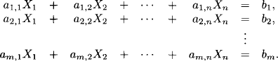
(9.2) ![]()
Then, the variable X1 is replaced by the right-hand expression in all other equations. After rearranging terms this results in the new system of linear equations
This is called a pivoting step with a1,1 as pivot element. Variable X1 is called the pivot variable and the first equation, where the pivot element is selected from, is called the pivot equation. It eliminates variable X1 and reduces the system of equations to a new system with one less variable and one less equation. The new system is equivalent to the old one in the following sense:
1. If (x1, x2, …, xn) is a solution to the original system, then (x2, …, xn) is a solution of the new system.
2. If (x2, …, xn) is a solution of the new system, then (x1, x2, …, xn) with
![]()
is a solution to the original system.
This procedure is called Gaussian variable elimination and can be repeated on the new system. In order to execute a pivot step on a variable Xi there must be at least one equation with a non-zero coefficient of Xi. If there is no such equation, Xi can be eliminated from the system without further actions. In fact, in this case Xi has zero coefficients in all equations which is tantamount to say that Xi does not appear in the system. So, Gaussian elimination permits to reduce the system stepwise by eliminating one variable after the other until only one variable remains. Several cases may arise during the elimination of variables: assume that the variables X1 to Xp have been successfully eliminated. Then, the following three cases may arise:
1. All coefficients on the left-hand side of the new system vanish, but on the right-hand side there is at least one element different from zero. In this case the system has no solution.
2. All coefficients on both sides of an equation vanish. Then, this equation can be eliminated. If no equations remain after elimination, then the variables Xp+1 to Xn can take arbitrary values.
3. There remains a non-vanishing system of linear equations with at least one equation less than the system before pivoting on Xp. Then, a next pivot step can be executed.
The first case identifies contradictions in the system. For this, we do not necessarily need to continue the pivoting process until all coefficients on the left-hand side of the system vanish. Instead, we may stop the process when the first equation arises, where all coefficient on the left-hand side vanish, but the right-hand side value is different from zero. These three cases solve the linear system in the following sense:
1. If case 1 occurs, the system has no solution.
2. In case 2 a certain number of variables X1, …, Xp can be expressed linearly by the remaining variables Xp+1, …, Xn. This determines the solution space.
3. All variables up to and including Xn-1 can be eliminated. Then Xn gets a fixed value in the last system, and a unique solution exists for the system. It can be found by backward substitution of the values of Xn, Xn-1, …
Note that which of the above cases arises does not depend on the order in which variables are eliminated.
The equations in the system after the first pivot step clearly show that original zero coefficients of certain variables may easily become non-zero in a pivot step. This is called a fill-in. The number of fill-ins depends on the choice of the pivot element or, in other words, there may be many fill-ins if the pivot element is not carefully chosen. Selection of the pivot element is partially a question of selecting elimination sequences of variables, but also of selecting the pivot equation. In the next section, we show how local computation allows to fix an elimination sequence such that fill-ins can be controlled and bounded. It should, however, be emphasized that limiting fill-ins is not the only consideration in selecting pivot elements. Numerical stability and the control of numerical errors are other important aspects that may be in contradiction to the minimization of fill-ins. The reader should keep this aspect in mind, although we here only focus on the limitation of fill-ins.
9.1.2 Fill-ins and Local Computation
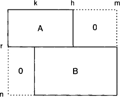
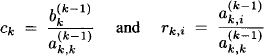
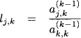
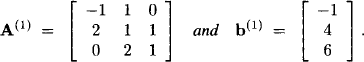
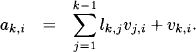
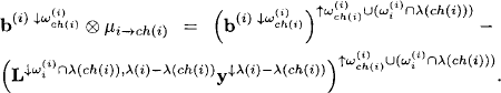
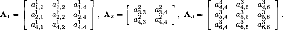
To discuss a concrete scenario we assume that in our system of linear equations (9.1) we have aj,i = 0 for all j = 1, …, r and i = h, …, n and also for j = r + 1, …, m and i = 1, …, k for some r < m and k < h < n. This corresponds to a decomposition of the system into a first subsystem of r equations, where only the variables X1 to Xh occur with non-zero coefficients and a second subsystem of m, − r equations where only the variables Xk+1 to Xn occur. The corresponding matrix decomposition is illustrated in Figure 9.1. We denote by A the r × h matrix of the first subsystem for the variables X1 to Xh and by B the (m − r) × (n − k) matrix of the second subsystem for the variables Xk+1 to Xn. It is already clear that if we select the pivot elements for the variables X1 to Xk in the first subsystem, then pivoting does not change the second subsystem, and in the first subsystem only the coefficients of the variables X1 to Xh change. So the zero-elements outside the two subsystems are maintained. This is how fill-ins are controlled by a decomposition.
Figure 9.1 A first decomposition of a system of linear equations into two subsystems and the associated zero-pattern of the coefficients.
If we want to eliminate the variables X1 to Xk, we have to distinguish two cases:
1. First, assume that r < k, i.e. there are less equations than variables to be eliminated. Then, we may eliminate at most r variables. Let us eliminate the variables in the order of their numbering X1, …, Xr. Then, it either turns out that the first subsystem has no solution, which implies that the whole system has no solution, or X1, …, Xr are at the end of the elimination process linearly expressed by the remaining variables Xr+1, …, Xh of the subsystem. We have for i = 1, …, r,
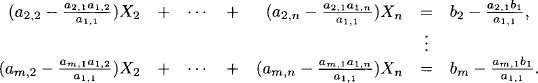
![]()
Here, the first variables Xr+1 to Xk can freely be chosen because they do not appear in the remaining second part of the system, whereas the last variables Xk+1 to Xh are determined by the second part of the system which can be solved independently of the first part.
2. In the second case, if k ≤ r, the elimination of the variables X1, X2, … may already show that the system has no solution. Otherwise, the variables X1 to Xk are eliminated from at least k equations of the first subsystem and there remain at most r − k equations containing only the variables Xk+1 to Xh. This system is added to the second subsystem which still contains only the variables Xk+1 to Xn. We thus obtain a new linear system for the variables Xk+1 to Xn. The eliminated variables X1, …, Xk are linearly expressed by the variables Xk+1, …, Xh. Once the second subsystem is solved for Xk+1, …, Xn we can backward substitute the solution into the expressions for X1, …, Xk.
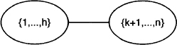
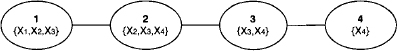
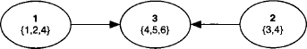
This describes a simple local computation scheme: the decomposition of the system can be represented by the two-node join tree of Figure 9.2. The variables of the first subsystem are covered by the label of the left-hand node and the variables of the second subsystem by the label of the right-hand node. The message sent from the left to the right node is obtained from eliminating all variables outside the intersection of the node labels. These are the variables X1 to Xk. The message is either empty or consists of the remaining system of the first subsystem after eliminating the variables X1 to Xk. If the elimination of the variables in the first subsystem already shows that the total system has no solution, then no message needs to be sent. Otherwise, the arriving message is simply added to the subsystem of the receiving node. Then, the variable elimination is continued in the new system until either a solution is found in the sense of the previous subsection, or it is seen that no solution exists. In the first case, assume that the variables Xk+1 to Xl are expressed by the remaining variables Xl+1, …, Xn. Note that since we did not make any assumption about the rank of the matrix, we cannot be sure that all this holds for all variables Xk+1 to Xh, but only for some l ≤ h. Then, the expression of the variables Xk+1 to Xl may be backward substituted into the expressions of the variables X1 to Xr if r < k, or to Xk obtained in the process of variable elimination in the first subsystem.
Figure 9.2 The join tree corresponding to the decomposition of Figure 9.1.
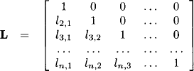
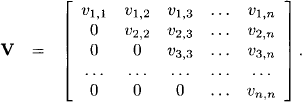
Let us point out more explicitly how the above scheme is connected to the local computation framework. We know from Section 7.2 that solution spaces of linear systems form a valuation algebra. Sets of equations provide a formal description of solution spaces and can therefore be considered as a representation of the latter. The domain of a set of equations consists of all variables that have at least one non-zero coefficient in this system. In the above description, we combined sets of equations by simple union. The original system therefore corresponds to the objective function and the knowledgebase factors are subsets of equations, whose union builds up the total system. This corresponds to the decomposition view presented in the introduction of this chapter. When producing such a decomposition from an existing system, we should keep the factor domains as small as possible. Otherwise, we will need large join tree nodes to cover these factors, which results in a bad complexity. In the case at hand, we can provide a factorization with minimum granularity where each factor contains exactly one equation. Then, the above procedure can be generalized as follows: we assume a covering join tree (V, E, λ, D) for the knowledgebase where each node i ![]() V contains a subsystem of linear equations whose variables are covered by the node label λ(i). This join tree decomposition reflects a certain pattern of zeros in the original total system. Note also that these systems may be empty on certain nodes, which mirrors the assignment of identity elements in Section 3.6. If we then execute the collect algorithm, the messages correspond to the description above. At the end of the message-passing, the root node contains the total system from which all variables outside the root label have been eliminated. We determine the remaining variables from this system and, if it exists, build the total solution by backward substitution. The depicted variable elimination process clearly maintains the pattern of zeros represented by the join tree decomposition. Consequently, join tree decompositions control fill-ins in general sparse systems of linear equations. This process will be formulated more precisely in Section 9.1.3 for the important case of regular systems that always provide a unique solution. There, we also point out that backward substitution in fact corresponds to the construction of solution configurations according to Section 8.2.1, see also Exercise H.1.
V contains a subsystem of linear equations whose variables are covered by the node label λ(i). This join tree decomposition reflects a certain pattern of zeros in the original total system. Note also that these systems may be empty on certain nodes, which mirrors the assignment of identity elements in Section 3.6. If we then execute the collect algorithm, the messages correspond to the description above. At the end of the message-passing, the root node contains the total system from which all variables outside the root label have been eliminated. We determine the remaining variables from this system and, if it exists, build the total solution by backward substitution. The depicted variable elimination process clearly maintains the pattern of zeros represented by the join tree decomposition. Consequently, join tree decompositions control fill-ins in general sparse systems of linear equations. This process will be formulated more precisely in Section 9.1.3 for the important case of regular systems that always provide a unique solution. There, we also point out that backward substitution in fact corresponds to the construction of solution configurations according to Section 8.2.1, see also Exercise H.1.
To identify the complexity of this approach, we consider a system that gives the most of work, i.e. a regular system of n variables and n equations. Eliminating one variable from this system takes a time complexity of ![]() (n2) and eliminating all variables is thus possible in
(n2) and eliminating all variables is thus possible in ![]() (n3). Backward substitution takes linear time for one variable and is repeated n times which result in
(n3). Backward substitution takes linear time for one variable and is repeated n times which result in ![]() (n2). Altogether, the time complexity of Gaussian elimination without taking care of fill-ins is
(n2). Altogether, the time complexity of Gaussian elimination without taking care of fill-ins is ![]() (n3). If local computation is applied, each join tree node contains a system of at most ω* + 1 variables, where ω* denotes the treewidth of the inference problem derived from the total system. The effort of eliminating one variable is
(n3). If local computation is applied, each join tree node contains a system of at most ω* + 1 variables, where ω* denotes the treewidth of the inference problem derived from the total system. The effort of eliminating one variable is ![]() ((ω* + 1)2), and a complete run of the collect algorithm that eliminates all variables takes
((ω* + 1)2), and a complete run of the collect algorithm that eliminates all variables takes
Backward substitution is performed n times with the equations that result from the variable elimination process and which contain at most ω* variables. We therefore obtain a time complexity of ![]() (nω*) for the complete backward substitution process. Because each node stores a matrix whose domain is bounded by the treewidth, we obtain the same bound as (9.3) for the space complexity. If the treewidth is small with respect to n, then big savings may be expected.
(nω*) for the complete backward substitution process. Because each node stores a matrix whose domain is bounded by the treewidth, we obtain the same bound as (9.3) for the space complexity. If the treewidth is small with respect to n, then big savings may be expected.
9.1.3 Regular Systems
In this section we examine more closely and more precisely the local computation scheme and the related structure of fill-ins for regular systems AX = b, where A is a regular n × n matrix. This assumption means that there is a unique solution to this system. In particular, we look at the fusion algorithm of Section 3.2.1 for computing the solution to this system. We choose an arbitrary elimination sequence for the n variables. By renumbering the variables and applying corresponding permutations of the columns of the matrix A, we may without loss of generality assume that the elimination sequence is (X1, X2, …, Xn). Further, by a well-known theorem of linear numerical analysis, it is also always possible to permute the rows of the matrix A such that in the sequence of the elimination of the variables X1, …, Xn all diagonal elements are different form zero (Schwarz, 1997). Again, without loss of generality, we may assume that the rows of A are already in the required order. This means that the following process of variable elimination works fine.
In the first step variable X1 is eliminated. Since by assumption a1,1 ≠ 0 we may solve the first equation for X1
![]()
where
for i = 2, …, n. Using this linear expression, we replace the variable X1 in the remaining equations to obtain
![]()
for j = 2, …, n with
Let us define
![]()
for j, i = 2, …, n. Then, the new system can be written as
![]()
By assumption ![]() is different from zero, variable X2 can be eliminated by solving the first equation of the new system and so forth. In the k-th step of this elimination process, k = 1, …, n, we similarly have
is different from zero, variable X2 can be eliminated by solving the first equation of the new system and so forth. In the k-th step of this elimination process, k = 1, …, n, we similarly have
where
for i = k + 1, …, n. Further, with
for j, i = k + 1, …, n, where
we get the system
![]()
In this process we define ![]() . For k = n − 1 it remains a simple system
. For k = n − 1 it remains a simple system
![]()
with one unknown that can easily be solved. By backward substitution for k = n − 2, …, 1, using equation (9.6), we obtain the solution of the regular system.
In order to study the control of fill-ins by local computation, we consider the join tree induced by the above execution of the fusion algorithm as described in Section 3.2.2. To each eliminated variable Xi corresponds a node i ![]() V in the join tree (V, E, λ, D) with a certain label λ(i)
V in the join tree (V, E, λ, D) with a certain label λ(i) ![]() D = P({1, …, n}). Let us now interpret the fusion algorithm as a message-passing scheme in this join tree according to Section 3.5. To start with, consider node 1 where the variable X1 is eliminated. Let
D = P({1, …, n}). Let us now interpret the fusion algorithm as a message-passing scheme in this join tree according to Section 3.5. To start with, consider node 1 where the variable X1 is eliminated. Let
![]()
define the index set of all equations which contain the variable X1. Only these equations are changed when variable X1 is eliminated. Further, let
![]()
be the set of variables that occur in the subset of equations with indices in ![]() (1). Note that the first equation is in
(1). Note that the first equation is in ![]() (1), since by assumption a1,1 ≠ 0. Hence, also the variable X1 is in the label λ(1) of node 1. When we now look at the elimination process of variable X1 according to the equations (9.4) and (9.5) above, then we remark that r1,i = 0 for i ∉ λ(1) and lj,1 = 0 for j ∉
(1), since by assumption a1,1 ≠ 0. Hence, also the variable X1 is in the label λ(1) of node 1. When we now look at the elimination process of variable X1 according to the equations (9.4) and (9.5) above, then we remark that r1,i = 0 for i ∉ λ(1) and lj,1 = 0 for j ∉ ![]() (1) and also
(1) and also
![]()
This shows that zeros in the first row and the first column of A are maintained when eliminating variable X1. Further, it exhibits the locality of the process by showing that only equations which contain variable X1 will change. The message sent to the child node ch(1) of node 1 in the join tree is determined by the coefficients
![]()
for j ![]()
![]() (1) − {1} and i
(1) − {1} and i ![]() λ(1) − {1}. These coefficients specify the new system of equations after elimination of variable X1. This process is repeated for variables Xk and nodes k for k = 1, …, n − 1. For node k of the join tree, where the variable Xk is eliminated, we define as above
λ(1) − {1}. These coefficients specify the new system of equations after elimination of variable X1. This process is repeated for variables Xk and nodes k for k = 1, …, n − 1. For node k of the join tree, where the variable Xk is eliminated, we define as above
![]()
for the equations containing variable Xk after k − 1 elimination steps and
![]()
for the variables contained in these equations. Again, by assumption, ![]() ≠ 0. Hence, the k-th. equation belongs to
≠ 0. Hence, the k-th. equation belongs to ![]() (k) and the variable Xk belongs to λ(k). So, we may eliminate variable Xk from the k-th equation. Similar to the first step, we remark that rk,i = 0 for i ∉ λ(k) and lj,k = 0 for j ∉
(k) and the variable Xk belongs to λ(k). So, we may eliminate variable Xk from the k-th equation. Similar to the first step, we remark that rk,i = 0 for i ∉ λ(k) and lj,k = 0 for j ∉ ![]() (k) and also
(k) and also
![]()
The message sent from node k to its child ch(k) is given by the coefficients
![]()
for j ![]()
![]() (k) − {k} and i
(k) − {k} and i ![]() λ(k) − {k}. The process stops at node n. This discussion permits to clarify how the zero-pattern of the matrix A is controlled and maintained by this fusion algorithm.
λ(k) − {k}. The process stops at node n. This discussion permits to clarify how the zero-pattern of the matrix A is controlled and maintained by this fusion algorithm.
Lemma 9.1 The k-th equation of the system AX = b is covered by some node i ≤ k of the join tree (V, E, λ, D). More precisely, there exists an index i ≤ k such that
![]()
Proof: Let i be the least index of the variables occurring in the k-the equation. Since the k-th equation contains no variables with indices h < i, we conclude that k ∉ ![]() (h) for h ≤ i and hence ak,l(i) = ak,l for l = 1, …, n and ak,i(i) = ak,i ≠ 0. So, the k-th equation belongs to
(h) for h ≤ i and hence ak,l(i) = ak,l for l = 1, …, n and ak,i(i) = ak,i ≠ 0. So, the k-th equation belongs to ![]() (i) and is therefore covered by λ(i).
(i) and is therefore covered by λ(i).
This result allows us to assign each equation k to some node i ≤ k of the join tree, and we have ak,h = 0 for h ∉ λ(i). This zero-pattern is maintained through the variable elimination process due to the remarks of the analysis above, i.e. ![]() = 0 for h ∉ λ(i) and l ≤ i.
= 0 for h ∉ λ(i) and l ≤ i.
To complete the description of the fusion algorithm in the case of a regular system of linear equations, we summarize it as a message-passing scheme: The system of equations assigned to the node k of the join tree is denoted by ![]() k for k = 1, …, n. Some of these systems may be empty. A system
k for k = 1, …, n. Some of these systems may be empty. A system ![]() k determines the affine space ψk of its solutions. If the system is empty, the affine space consists of all possible vectors. In other words, ψk is then the neutral valuation in the information algebra of affine spaces. The problem of finding the solution to the system AX = b can then be written for k = 1, …, n as the inference problem
k determines the affine space ψk of its solutions. If the system is empty, the affine space consists of all possible vectors. In other words, ψk is then the neutral valuation in the information algebra of affine spaces. The problem of finding the solution to the system AX = b can then be written for k = 1, …, n as the inference problem
![]()
Given the uniqueness of the solution, each such projection is just a number.
Now, the fusion algorithm is described in terms of the information elements ψk as follows: at step 1, node 1 sends the message
![]()
to its child node ch(1). This is done by transforming the systems of equations ![]() 1 according to the above procedure, i.e. by solving the first equation with respect to X1 and replacing the variable X1 in the remaining equations of
1 according to the above procedure, i.e. by solving the first equation with respect to X1 and replacing the variable X1 in the remaining equations of ![]() 1. The resulting system is denoted by
1. The resulting system is denoted by ![]() 1→ch(1) and represents the message μ1→ch(1). The message is combined to the content of node ch(1) to get
1→ch(1) and represents the message μ1→ch(1). The message is combined to the content of node ch(1) to get
![]()
This new system is simply represented by
![]()
More generally, let ψi(k) be the information element on node i before step k of the fusion algorithm. We therefore have ψi(1) = ψi. The associated system of equations is denoted by ![]() i(k). At step k, node k sends the message
i(k). At step k, node k sends the message
![]()
to node ch(k) by solving the first equation of the system ![]() k(k) with respect to Xk and replacing the variable Xk in the remaining equations, which gives the system
k(k) with respect to Xk and replacing the variable Xk in the remaining equations, which gives the system ![]() k→ch(k) representing the message. This message is added to the system in the child node ch(k) to yield
k→ch(k) representing the message. This message is added to the system in the child node ch(k) to yield
![]()
All other nodes remain unchanged, i.e. ![]() for i ≠ ch(k). This process is repeated for k = 1, …, n − 1. At the end, the root node n contains the valuation
for i ≠ ch(k). This process is repeated for k = 1, …, n − 1. At the end, the root node n contains the valuation ![]() ↓(Xn) which is represented by the system
↓(Xn) which is represented by the system
This is the end of the fusion algorithm interpreted as message-passing scheme, or equivalently, of the collect algorithm as described in Section 3.8, executed on the particular join tree that is induced by the fusion algorithm.
Since we are dealing with an idempotent valuation algebra, we can use the corresponding architecture from Section 4.5 for the distribute phase to compute the complete solution ![]() →{Xi} for all i = 1, …, n. We first transform equation (9.10) on the node n into the equivalent form
→{Xi} for all i = 1, …, n. We first transform equation (9.10) on the node n into the equivalent form
from which we determine the solution value
![]()
This in fact defines the single-point affine space ![]() →{Xn} = {xn}. Observe now that if n − 1 is a neighbor to node n such that ch(n − 1) = n, it follows by the construction of the join tree from the fusion algorithm that λ(n − 1)
→{Xn} = {xn}. Observe now that if n − 1 is a neighbor to node n such that ch(n − 1) = n, it follows by the construction of the join tree from the fusion algorithm that λ(n − 1) ![]() λ(n) = λ(n − 1) − {Xn-1} = {Xn}. So, the message sent from node n to node n − 1 in the distribute phase is
λ(n) = λ(n − 1) − {Xn-1} = {Xn}. So, the message sent from node n to node n − 1 in the distribute phase is
![]()
This means that equation (9.11) is added to the system ![]() containing the equation
containing the equation
besides possibly a second system that represents the message from node n − 1 to n in the collect phase. This second system is redundant with the equation (9.11) and can be eliminated. Finally, the solution xn from equation (9.11) can be introduced into (9.12) to yield the solution value for Xn-1 determining the affine space ![]() →{Xn-1}. In the general step of the distribute phase, node k receives a message
→{Xn-1}. In the general step of the distribute phase, node k receives a message
![]()
from its child node ch(k). By the induction assumption this message is a single-point affine space given by the solution values x1 for i ![]() λ(k) − {k}. The system of equations on node k contains the equation
λ(k) − {k}. The system of equations on node k contains the equation
![]()
The solution values contained in the message are introduced into this equation to get the solution value for Xk,
![]()
So, by induction, distribute corresponds to the construction of the solution values of the variables Xk on the nodes k of the join tree by backward substitution. This is in fact a consequence of the theory of solution construction developed in Chapter 8 applied to context valuation algebras. In Exercise H.4 we proposed to define solution sets in context valuation algebras by their associated set of models. The computations in the relational algebra of solution sets performed by the solution construction algorithms of Section 8.2 therefore correspond to computations in the context valuation algebra itself. Hence, the above execution of the idempotent distribute phase coincides with the application of the generic solution construction procedure from Section 8.2.3. We continue this discussion in Section 9.2 and Section 9.3.2, where other valuation algebra are studied that do not belong to the class of context valuation algebras. There, the solution construction procedures will be applied explicitly.
This completes the picture of the solution process as a message-passing procedure on the join tree induced by the fusion algorithm. In particular, the discussion shows that locality as represented by the join tree is also maintained during the distribute phase. It is important to understand that a similar process can be executed on an arbitrary join tree, where λ(k) ![]() λ(ch(k)) = λ(k) − {Xk} does not necessarily hold. Here, we have chosen the very particular join tree of the fusion algorithm for illustration purposes, i.e. exactly one variable is eliminated from the equation system between two neighboring join tree nodes. It follows a numerical example:
λ(ch(k)) = λ(k) − {Xk} does not necessarily hold. Here, we have chosen the very particular join tree of the fusion algorithm for illustration purposes, i.e. exactly one variable is eliminated from the equation system between two neighboring join tree nodes. It follows a numerical example:
Example 9.1 Consider a regular 4 × 4 matrix A and a corresponding vector b,

We solve the linear system AX = b by elimination of the variables X1, X2 and X3 in this order. Eliminating X1 yields the following new matrix A(1) and the new right-hand side vector b(1):
We remember also the non-zero r- and l-elements r1,2 = 1 and l2,1 = 2. Next, we eliminate X2 and obtain
![]()
In addition we have r2,3 = −1 and l3,2 = −2. It remains to eliminate X3 giving
![]()
with l4,3 = 2/3 and r3,4 = ![]() . We can now solve the equation
. We can now solve the equation
![]()
for X4 and obtain the solution value x4 = 14.
Figure 9.3 shows the join tree induced by the fusion algorithm described above. We may assign the first two equations to the left-most node and the last two equations to the second node from the left. Eliminating the variable X1 generates the equation
Figure 9.3 The join tree induced by the variable elimination in Example 9.1.
![]()
as the message sent to the next node. There, this equation is added to the two equations already hold by this node. This yields the linear system defined by the matrix A(1) and the vector b(1). Next, eliminating the variable X2 generates the system described by the matrix A(2) and the vector b(2) as the message to be sent from the second to the third node. Since the system contained in the third node is empty, the node content becomes equal to the received message. Finally, eliminating the variable X3 generates the equation (1/3)X4 = 14/3 as the message sent to the fourth node. Again, the content of node 4 is an empty system such that the received message directly becomes the new node content.
Now, the distribute phase starts by solving the equation of node 4, which gives us the solution value x4 = 14 as remarked above. Node 4 sends this solution value back to node 3, where it can substitute the variable X4. Using the first equation of the system defined by A(2) and b(2) on this node, we can solve for X3 to obtain X3 = 2/3 − (1/3)x4 = −4. This is the value sent back to node 2, where it can be used to determine the solution value of X2 using the first equation of the system on this node, x2 = 1 + x3 = −3. Finally, this values is sent back to node 1, where we get from the first equation x1 = 2 − x2 = 5. This constitutes the totality of the unique solution of the system AX = b. Note that in the whole process, at each step only the variables belonging to the label of the current join tree node are involved. This shows the locality of the solution process.
In the next section we study a variant of this process, which has advantages if the system of equations AX = b must be solved for different vectors b. By memorizing certain intermediate factors derived from the matrix A in the first run of the above algorithm, we obtain a factorization of A into an upper and a lower triangular matrix. If later another equation system with the same matrix must be solved, only the computations with respect to the new vector must be repeated. This considerably simplifies the computations of the involved local computation messages.
9.1.4 LDR-Decomposition
Let us review the process of Gaussian variable elimination described in Section 9.1.3. From the recursive definition in equation (9.8) we derive
![]()
for 1 ≤ k ≤ i, if we define vk,i = ![]() . This implies that
. This implies that
If we set lk,k = 1, we may also write
This can also be expressed by the matrix product
![]()
where L is a lower triangular und R an upper triangular matrix,
and
This representation is called LV-decomposition of the matrix A. We remark that the vk,i used here are closely related to the elements rk,i in equation (9.7). We have
Therefore, if we define the diagonal matrix D with elements dk,k = 1/vk,k on the diagonal and zeros otherwise, and further the upper triangular matrix

then we have the representation
![]()
This is called LDR-decomposition of the matrix A.
We may neglect the right-hand side of the system AX = b in the fusion algorithm described in the previous Section 9.1.3 and only compute the elements lk,i, rk,i and ![]() that depend on the matrix A. If we relate these elements to the join tree induced by the fusion algorithm, we remind that rj,i = 0 for i ∉ λ(j) and lk,j = 0 for j ∉
that depend on the matrix A. If we relate these elements to the join tree induced by the fusion algorithm, we remind that rj,i = 0 for i ∉ λ(j) and lk,j = 0 for j ∉ ![]() (j). Thus, the two matrices L and R maintain the zero-pattern described by the join tree. The computation of the LDR-decomposition in the fusion algorithm can be interpreted as a compilation of the matrix A, which can then be used to solve AX = b for different vectors b. This will be shown next.
(j). Thus, the two matrices L and R maintain the zero-pattern described by the join tree. The computation of the LDR-decomposition in the fusion algorithm can be interpreted as a compilation of the matrix A, which can then be used to solve AX = b for different vectors b. This will be shown next.
Given some vector b and the LV- or LDR-decomposition of the matrix A, we solve the system AX = b by first solving LY = b, yielding the solution y, and then VX = DRX = y. This solution process is simple, since both matrices L and V are triangular: We first solve the system LY = b by executing the collect algorithm on the join tree. In fact, starting with node 1 we directly obtain the solution value y1 = b1 from the first equation Y1 = b1. We introduce this value into the equations j ![]()
![]() (1) − {1} and obtain the new system
(1) − {1} and obtain the new system
![]()
Defining ![]() = bj − lj,1b1, the message sent to the child node ch(1) is the set
= bj − lj,1b1, the message sent to the child node ch(1) is the set
![]()
This defines the new lower triangular system after elimination of variable Y1. In the k-th step, the equation for Yk on the node k is Yk = ![]() . The solution value yk = bk(k-1) is introduced into the equations j
. The solution value yk = bk(k-1) is introduced into the equations j ![]()
![]() (k) − {k} to obtain
(k) − {k} to obtain
![]()
So, the message sent to the child node ch(k) is the set
![]()
with bk(k) = bj(k-1) − lj,kbk(k-1). In this way, the solution yk for k = 1, …, n is obtained. It is important to remark that in the general case, the collect algorithm only computes the solution for the variable Yn in the root node, and the values for the remaining variables are found by backward substitution in the distribute phase. In the case at hand, we are dealing with triangular systems and therefore obtain all solutions y of the system LY = b already from the collect algorithm.
In a second step, we execute the distribute algorithm to solve the system VX = DRX = y, respectively RX = D−1y. The root node n contains the equation Xn = yn/dn,n from which we determine the solution value xn = yn/dn,n. This value is sent to node n − 1 and replaces there the variable Xn in the equations from RX = D−1y that are contained in the node n − 1. More precisely, we compute for
![]()
for j ![]() λ(n − 1), according to equation (9.12). In the general case, node k receives a message from node ch(k), which consist of
λ(n − 1), according to equation (9.12). In the general case, node k receives a message from node ch(k), which consist of
![]()
for j ![]() ≤(k). Altogether, this permits to solve the triangular system of equations on the node k for k = n, …, 1.
≤(k). Altogether, this permits to solve the triangular system of equations on the node k for k = n, …, 1.
We again point out that the solution of AX = b for an arbitrary, regular matrix A required in the previous section a complete run of the collect and distribute algorithm. But if we dispose of an LDR-decomposition of A, we may solve the system LY = b with a single run of the collect algorithm, because the involved matrix L is lower triangular. Likewise, we directly obtain the solution to the system DR = y by a single run of the distribute algorithm, because the matrix DR is upper triangular. This symmetry between the application of collect and distribute is worth noting.
We apply this compilation approach to Example 9.1 above:
Example 9.2 In Example 9.1 we determined the elements of the matrices L and R,
We remark how the zero-pattern controlled by the join tree of Figure 9.3 is still reflected, both in the matrix L as well as in the matrix R. With the diagonal matrix below we obtain the LDR-decomposition A = LDR:
In the first step, we solve the system LY = b, where b is given in Example 9.3. We again assign the first two equations of this system to the first join tree node and the last two equations to the second node to control fill-ins. In the first node, we obtain y1 = 2 and introduce this value into the second equation, whose right-hand side becomes b2(2) = b2 − l2,1y1 = −1. This value is sent to node 2, where now the solution value y2 = b2(1) = −1 is obtained. Also, node 2 computes the message b3(3) = b3 − l3,2y2 = 2 and sends it to node 3. Node 3 computes y3 = 2 and sends the message b4(3) = b4 − l4,3y3 = 14/3 to node 4, where we finally obtain y4 = 14/3.
The solution of RX = D−1y by the distribute algorithm, using the values y computed in the collect phase, is initiated by the root node 4. We obtain on node 4 the value x4 = y4/d4,4 = 14. This value is sent to node 3, where we obtain x3 = y3/d3,3 − r3,4x4 = −4 and send this message to node 2. Continuing this process, we obtain x2 = y2/d2,2 − r2,3x3 = −3 in node 2 and x1 = y1/d1,1 − r1,2x2 = 5 in node 1. This terminates the distribute phase. We note that on all nodes j only variables from the node label λ(j) are involved.
This ends our first discussion of regular systems. An important special case of regular systems is provided by symmetric, positive definite systems. They allow to refine the present approach as shown in the following section.
9.2 SYMMETRIC, POSITIVE DEFINITE MATRICES
The method of LDR-decomposition presented in the previous section becomes especially interesting in the case of linear systems with symmetric, positive definite matrices. Such systems arise frequently in electrical network analysis, analysis of structural systems and hydraulic problems. Further, they arise in the classical method of least squares, which will be discussed in Section 9.2.5 as an application of the results developed here. In all these cases, the exploitation of sparsity is important. However, it turns out that in the case of systems of linear equations with symmetric, positive definite matrices, the underlying algebra of affine solution spaces is of less interest and can be replaced by another valuation algebra. We first introduce this algebra, which interestingly is closely related to the valuation algebra of Gaussian potentials introduced in Instance 1.6. The reason for this is elucidated in Section 9.2.5, where systems of linear equations with symmetric, positive definite matrices are related to statistical problems.
9.2.1 Valuation Algebra of Symmetric Systems
To put the discussion into the general framework of valuation algebras, we consider variables X1, …, Xn together with the associated index set r = {1, …, n}. Vectors of variables X, as well as matrices A and vectors b then refer to certain subsets s ⊆ r. For instance, a system AX = b is said to be an s-system, if X is the variable vector whose components Xi have indices in s ⊆ r, A is a symmetric, positive definite s × s matrix and b is an s-vector. Such systems are fully determined by the pair (A, b) where A is an s × s matrix, b an s-vector for some s ⊆ r. These are the elements of the valuation algebra to be identified. Let Φs be the set of all pairs (A, b) relative to some subset s ⊆ r and define
![]()
By convention, we define for the empty set ![]() . The label of a pair (A, b) is defined as d(A, b) = s, if (A, b)
. The label of a pair (A, b) is defined as d(A, b) = s, if (A, b) ![]() Φs.
Φs.
In order to define the operations of combination and projection for elements in Φ, we first consider variable elimination in the system AX = b. Suppose (A, b) ![]() Φs, i.e. the system is over variables in s, and assume t ⊆ s. We want to eliminate the variables in the index set s − t. For this purpose, we decompose A as follows:
Φs, i.e. the system is over variables in s, and assume t ⊆ s. We want to eliminate the variables in the index set s − t. For this purpose, we decompose A as follows:
![]()
The system AX = b can then be written as
![]()
Solving the first part for X↓s − t and substituting this in the second part leads to the reduced system for X↓t
![]()
Here we use the fact that any diagonal submatrix of a symmetric, positive definite matrix is regular. We define
and remark that ![]() is still symmetric, positive definite.
is still symmetric, positive definite.
Theorem 9.1 If x is the unique solution of AX = b, then x↓t is the unique solution to ![]() . Conversely, if y is the unique solution of
. Conversely, if y is the unique solution of ![]() and
and
![]()
then (x, y) is the unique solution of AX = b.
Proof: The proof is straightforward, using the definitions of ![]() . Since x is a solution of AX = b, it holds that
. Since x is a solution of AX = b, it holds that
![]()
hence
![]()
This proves the first part of the theorem. The second part follows from the first subsystem above, if x↓s-t is replaced by x and x↓t by y and if it is multiplied on both sides by (A↓s-t,s-t)−1.
This theorem justifies to define the operation of projection for elements in Φ by
for t ⊆ d(A, b). It is well-known in matrix algebra that ![]() may also be written as
may also be written as
![]()
A proof can for example be found in (Harville, 1997).
Next, consider two systems A1X1 = b1 and A2X2 = b2. What is a sensible way to combine these two systems into a new system? Clearly, taking simply the union of both systems as we did so far with systems of linear equations makes no sense, because the matrix of the combined system will no more be symmetric. Moreover, the combined system will most of the time have no solution anymore. We propose alternatively to add the matrices and the right-hand vectors component-wise. More precisely, we define for d(A1, b1) = s and d(A2, b2) = t,
At this point, the proposed definition is rather ad hoc. It will be justified by the success of local computation and even more strongly by a semantical interpretation given in the following Section 9.2.5. For the time being, the question is whether (Φ, D) together with the operations of labeling, projection and combination satisfies the axioms of a valuation algebra. Instead of verifying the axioms directly, we consider the mapping (A, b) ![]() (A, u), where u = A−1b. Let ψ be the set of all pairs (A, u), where A is a symmetric, positive definite s × s matrix and u an s-vector. This mapping is a surjection between Φ and ψ. We next look at how combination and projection in Φ is mapped to ψ. Let (A1, b1) and (A2, b2) belong to Φ with labels s and t, respectively. Then, by the definition of combination above, (A1, b1)⊗(A2, b2) = (A, b) with
(A, u), where u = A−1b. Let ψ be the set of all pairs (A, u), where A is a symmetric, positive definite s × s matrix and u an s-vector. This mapping is a surjection between Φ and ψ. We next look at how combination and projection in Φ is mapped to ψ. Let (A1, b1) and (A2, b2) belong to Φ with labels s and t, respectively. Then, by the definition of combination above, (A1, b1)⊗(A2, b2) = (A, b) with
![]()
Hence, (A1, b1) ⊗ (A2, b2) maps to (A, u) with
where u1 = A1−1b1 and u1 = A2−1b2. Consequently, a combination of two elements in Φ is mapped as follows to an element in ψ
![]()
with
![]()
and
![]()
Turning to projection, let (A, b) be an element in Φ with domain s, which is mapped to (A, u) with u = A−1b. If t ⊆ s, then (A, b)↓t represents the system ![]() with the unique solution u↓t as a consequence of Theorem 9.1. This means that (A, b)↓t maps to
with the unique solution u↓t as a consequence of Theorem 9.1. This means that (A, b)↓t maps to
![]()
where
![]()
We thus have the following projection rule in ψ:
![]()
We observe that combination and projection in ψ correspond exactly to the operations of Gaussian potentials introduced in Instance 1.6 and we therefore know that ![]() ψ, D
ψ, D![]() forms a valuation algebra. Moreover, due to the introduced mapping,
forms a valuation algebra. Moreover, due to the introduced mapping, ![]() ψ, D
ψ, D![]() and
and ![]() ψ, D
ψ, D![]() are isomorphic which implies that
are isomorphic which implies that ![]() Φ, D
Φ, D![]() is a valuation algebra. We proved the following theorem:
is a valuation algebra. We proved the following theorem:
Theorem 9.2 The algebra of linear systems with symmetric, positive definite matrices is isomorphic to the valuation algebra of Gaussian potentials.
Let us have a closer look at the combination of (A1, b1) and (A2, b2) with d(A1, b1) = s and d(A2, b2) = t. If X denotes an (s ∪ t) variable vector, these valuations represent the systems A1X↓s = b1 and A2X↓t = b2 with symmetric, positive definite matrices. We consider the system AX = b which is represented by (A1, b1) ⊗ (A2, b2) such that
![]()
In order to compute the solution to the system AX = b, we proceed in two steps by first projecting to t, i.e. eliminating the variables X↓s-t, and then solving the system ![]() . This is justified by Theorem 9.1. We decompose the matrices and vectors according to the sets s − t, s
. This is justified by Theorem 9.1. We decompose the matrices and vectors according to the sets s − t, s ![]() t and t − s and write the system as
t and t − s and write the system as
Eliminating the variables X↓s − t means to solve the first subsystem for the variables X↓s-t and to substitute the solution into the other equations, which gives the system
![]()
Note that this system is represented by either
(9.16) ![]()
This illustrates the combination axiom and shows how local computation can be applied to symmetric, positive definite systems. If the second representation is used, then the variables X↓s-t in the first system are eliminated and the result is combined to the second system. It would be reasonable to apply the local computation methods of Section 9.1.2 and 9.1.3 for the variable elimination process. This however is not possible because idempotency does not hold anymore in this algebra. Symmetric, positive definite systems only form a valuation algebra but not an information algebra. For local computation, this means that we must apply the Shenoy-Shafer architecture. However, Theorem 9.1 offers an alternative possibility based on solution construction which comes near to idempotency. This is exploited in the following section, and variable elimination and LDR-decomposition with symmetric systems is examined in Section 9.2.3.
9.2.2 Solving Symmetric Systems
We now return to local computation as a means to control fill-ins. Note that zero-patterns in a symmetric matrix are symmetric too. Consequently, symmetric decompositions of the matrix A as shown in Figure 9.1 are not possible. This implies that the underlying valuation algebra of affine spaces introduced in Section 7.2 and used so far is no longer of interest. In other words, combination as intersection or join of affine spaces does not really reflect the natural decomposition of symmetric systems. Instead, this is achieved by adding symmetric, positive definite matrices as showed in the foregoing section. The corresponding algebra will now be used to control fill-ins.
Consider a join tree (V, E, λ, D) with the labeling function λ: V → D = P(r) for r = {1, …, n}. We number the nodes from 1 to m = |V| and assume that any node i ![]() V in this join tree covers a pair
V in this join tree covers a pair ![]() i = (Ai, bi) with ωi = d(
i = (Ai, bi) with ωi = d(![]() i). They consist of a symmetric, positive definite ωi × ωi matrix Ai and an ωi-vector bi. We further assume that ωi
i). They consist of a symmetric, positive definite ωi × ωi matrix Ai and an ωi-vector bi. We further assume that ωi ![]() λ(i) and ω1 ∪ … ∪ ωm = r. In other words,
λ(i) and ω1 ∪ … ∪ ωm = r. In other words, ![]() i are elements of the valuation algebra introduced in Section 9.2.1 and (V, E, λ, D) is a covering join tree for the factorization
i are elements of the valuation algebra introduced in Section 9.2.1 and (V, E, λ, D) is a covering join tree for the factorization
according to Definition 3.8. As usual, the nodes of the join tree are numbered such that if node j is on the path form node i to node m, then i < j. We will see in Section 9.2.4 how such decompositions can be produced, and it will be shown in 9.2.5 that factorizations of symmetric, positive definite systems may also occur naturally in certain applications. The objective function ![]() represents the symmetric, positive definite system AX = b, where
represents the symmetric, positive definite system AX = b, where
![]()
and
![]()
The join tree exhibits the sparsity of the matrix A. We have aj,h = 0, if j and h do not belong both to some ωi. Its zero-pattern is denoted by the set
Given a factorized system ![]() = (A, b) =
= (A, b) = ![]() 1 ⊗ … ⊗
1 ⊗ … ⊗ ![]() m and some covering join tree, we next focus on the solution process using local computation. As mentioned above, this algebra is fundamentally different from the algebra of affine spaces and does not directly yield solution sets. Instead, we aim at first executing a local computation scheme and later build the solution x = A−1b using a generic solution construction algorithm from Chapter 8. Hence, we start by introducing a suitable notion of configuration extension sets for symmetric, positive define systems, motivated by Theorem 9.1: For a t-vector of real numbers x,
m and some covering join tree, we next focus on the solution process using local computation. As mentioned above, this algebra is fundamentally different from the algebra of affine spaces and does not directly yield solution sets. Instead, we aim at first executing a local computation scheme and later build the solution x = A−1b using a generic solution construction algorithm from Chapter 8. Hence, we start by introducing a suitable notion of configuration extension sets for symmetric, positive define systems, motivated by Theorem 9.1: For a t-vector of real numbers x, ![]() = (A, b) and t ⊆ d(
= (A, b) and t ⊆ d(![]() ) we define
) we define
For later reference we prove the following property:
Lemma 9.2 Assume ![]() 1 = (A, b1) and
1 = (A, b1) and ![]() 2 = (A, b2) with d(
2 = (A, b2) with d(![]() 1) = d(
1) = d(![]() 2) = s and t ⊆ u ⊆ s. If
2) = s and t ⊆ u ⊆ s. If
![]()
then it holds for all t-vectors x that
![]()
Proof: By equation (9.19) and ![]() we have for i = 1, 2
we have for i = 1, 2
The statement of the lemma then follows directly from:
Based on this lemma, we show that the definition of equation (9.19) complies with the general definition of configuration extension sets in Section 8.1.
Theorem 9.3 Solution extension sets in valuation algebras of symmetric, positive definite systems satisfy the property of Definition 8.1, i.e. for all ![]() = (A, b)
= (A, b) ![]() Φ with t ⊆ u ⊆ s = d(
Φ with t ⊆ u ⊆ s = d(![]() ) and all t-vectors x we have
) and all t-vectors x we have
![]()
Proof: If x is the partial solution to the system ![]() = (A, b), then the above statement follows directly from Theorem 9.1. In the following proof, we consider an arbitrary t-vector x and determine a new system
= (A, b), then the above statement follows directly from Theorem 9.1. In the following proof, we consider an arbitrary t-vector x and determine a new system ![]() 1 = (A, b1) to which x is the partial solution. The statement then holds for x with respect to this new system, and if
1 = (A, b1) to which x is the partial solution. The statement then holds for x with respect to this new system, and if ![]() 1 is chosen in such a way that Lemma 9.2 applies, then the statement also holds for x with respect to the original system
1 is chosen in such a way that Lemma 9.2 applies, then the statement also holds for x with respect to the original system ![]() . Hence, let x be an arbitrary t-vector. We consider the new system
. Hence, let x be an arbitrary t-vector. We consider the new system ![]() 1 = (A, b1) with
1 = (A, b1) with
![]()
and determine ![]() such that x is the solution to
such that x is the solution to ![]() , i.e.
, i.e.
![]()
and therefore
![]()
Since x is the solution to (A, b1)→t, it follows from Theorem 9.1 that (y, x) with
![]()
is the solution to the system (A, b1). We thus have
![]()
as a consequence of Lemma 9.2. Then, since (y,x) is the solution to (A,b1), it follows from Theorem 9.1 that (y↓u−t, x) is the solution to (A, b1)↓u. Hence,
![]()
by Lemma 9.2. Finally, since ![]() is the solution to (A, b1)↓u it again follows from Theorem 9.1 that (y↓u−t,x) is the solution to (A, b1). We have
is the solution to (A, b1)↓u it again follows from Theorem 9.1 that (y↓u−t,x) is the solution to (A, b1). We have
![]()
Altogether, this show that for an arbitrary t-vector x we have
![]()
Next, we specialize general solution sets from Definition 8.2 to symmetric, positive definite systems. For ![]() = (A, b)
= (A, b) ![]() Φ and t =
Φ and t = ![]() , it follows from equation (9.19) that
, it follows from equation (9.19) that
(9.20) ![]()
This shows that c![]() indeed corresponds to the singleton set of the unique solution x = A−1b to the symmetric, positive definite system AX = b. We therefore conclude that the generic solution construction procedure of Section 8.2.1 could be applied to build c
indeed corresponds to the singleton set of the unique solution x = A−1b to the symmetric, positive definite system AX = b. We therefore conclude that the generic solution construction procedure of Section 8.2.1 could be applied to build c![]() based on the results of a multi-query local computation scheme. However, the same is also possible using the results of a single-query architecture only. This follows by verifying the property of Theorem 8.3:
based on the results of a multi-query local computation scheme. However, the same is also possible using the results of a single-query architecture only. This follows by verifying the property of Theorem 8.3:
Lemma 9.3 Symmetric, positive definite systems satisfy the property that for all ψ1, ψ2 ![]() Φ with d(ψ1) = s, d(ψ2) = t, s ⊆ u ⊆ s ∪ t and u-vector x we have
Φ with d(ψ1) = s, d(ψ2) = t, s ⊆ u ⊆ s ∪ t and u-vector x we have
![]()
Proof: We observe the following identities for ψ1 = (A1, b1) and ψ2 = (A2, b2):
![]()
and similarly
![]()
It then follows that
Hence, given the results of a single-query local computation architecture, we may apply Algorithm 8.4 to build the unique solution x = A−1b of a factorized system ![]() = (A, b) =
= (A, b) = ![]() 1 ⊗ … ⊗
1 ⊗ … ⊗ ![]() m with
m with ![]() i = (Ai, bi) for i = 1, …, m. At this point, we should remember that the valuation algebra of symmetric, positive definite systems is isomorphic to the valuation algebra of Gaussian potentials and does not provide neutral elements; see Instance 3.5. Hence, the domain ωi = d(
i = (Ai, bi) for i = 1, …, m. At this point, we should remember that the valuation algebra of symmetric, positive definite systems is isomorphic to the valuation algebra of Gaussian potentials and does not provide neutral elements; see Instance 3.5. Hence, the domain ωi = d(![]() i) of node i
i) of node i ![]() V in the join tree does not necessarily correspond to the node label λ(i). We only have ωi ⊆ λ(i). Consequently, we must choose the generalized collect algorithm from Section 3.10 to explain the message-passing view of this local computation based solution. The run of this algorithm followed by the solution construction process is delineated next, using the notation of equation (3.42) from Section 3.10.
V in the join tree does not necessarily correspond to the node label λ(i). We only have ωi ⊆ λ(i). Consequently, we must choose the generalized collect algorithm from Section 3.10 to explain the message-passing view of this local computation based solution. The run of this algorithm followed by the solution construction process is delineated next, using the notation of equation (3.42) from Section 3.10.
At step i = 1, …, m −1, node i sends the message
![]()
to its child node ch(i), where the message is combined with the current node content
![]()
The domain of the node content updates to:
![]()
For all other nodes j ≠ ch(i) we set
![]()
with
![]()
for all i = 1, …, m. We now add an additional step that is not part of the general collect algorithm. When node i computes the message for its child node, it has to eliminate the variables
from its node content. This equality is due to Lemma 4.2. The eliminated variables satisfy the system
For later use in the solution construction phase, we store in node i the matrices on the right-hand side of the equation. This is the only modification with respect to the generalized collect algorithm. If we repeat this process up to i = m, we obtain on node m the pair
![]()
as a consequence of Theorem 3.7. The content of node m at the end of the collect phase represents the symmetric system
![]()
Solving this system gives us the partial solution set ![]() , as a consequence of Lemma 9.20 and Lemma 8.1. We now follow the solution construction algorithm of Section 8.2.3 starting in the root node m. At step i = m −1, …, 1 node i
, as a consequence of Lemma 9.20 and Lemma 8.1. We now follow the solution construction algorithm of Section 8.2.3 starting in the root node m. At step i = m −1, …, 1 node i ![]() V receives the partial solution set
V receives the partial solution set
![]()
from its child node ch(i). Using the matrices stored in (9.22), node i computes
(9.23) ![]()
to obtain the partial solution x↓λ(i) = ![]() with respect to its proper node label. At the end of the solution construction process, each node i
with respect to its proper node label. At the end of the solution construction process, each node i ![]() λ(i) contains the solution x to the system AX = b projected to its node label, and the complete solution x can simply be obtained by assembling these partial solutions. This shows how factorized, symmetric, positive definite systems are solved using local computation. The sparsity reflected by the join tree is maintained all the time. A very similar scheme for the computation of solutions in quasi-regular semiring systems will be presented in Section 9.3.2. Here, we next focus on the adaption of LDR-decomposition to symmetric, positive definite systems.
λ(i) contains the solution x to the system AX = b projected to its node label, and the complete solution x can simply be obtained by assembling these partial solutions. This shows how factorized, symmetric, positive definite systems are solved using local computation. The sparsity reflected by the join tree is maintained all the time. A very similar scheme for the computation of solutions in quasi-regular semiring systems will be presented in Section 9.3.2. Here, we next focus on the adaption of LDR-decomposition to symmetric, positive definite systems.
9.2.3 Symmetric Gaussian Elimination
Consider again a system AX = b, where A is a symmetric, positive definite n × n matrix, and X and b are vectors with corresponding dimensions. Since positive definite systems are always regular, we could apply the local computation scheme based on the LDR-decomposition from Section 9.1.3, if we have to solve this system multiple times for different vectors b. However, here we are dealing with a different valuation algebra such that parts of this discussion must be revisited. Moreover, the approach presented in this section does not only exploit the sparsity of the system, but also benefits from the symmetry in the matrix A. Because this matrix is regular, we can use any variable elimination sequence in the Gaussian method to solve the system. As in Section 9.1.3, we renumber the variables such that they are eliminated in the order X1, …, Xn. We only need to permute the columns and the rows of the matrix A accordingly. By the symmetry of the matrix, the same permutation must be used for both columns and rows. In addition, it follows by symmetry that the LDR-decomposition satisfies R = LT such that
![]()
For positive definite matrices, D has positive diagonal entries. It also holds that
![]()
where G = LD1/2. This decomposition is due to Choleski (Forsythe & Moler, 1967).
The symmetry of the matrix A can be exploited for the elimination of variables, where it is now sufficient to store the lower (or upper) half of the matrix A and all derived matrices. Then, equation (9.9) still applies: For j, i = k + 1, …, n we have
and according to equation (9.8) also
![]()
Only the elements ![]() for k ≤ j ≤ i must be computed due to the symmetry in the matrix A. We again remark that in a symmetric, positive definite matrix the diagonal elements dk,k are positive in each step k = 1, …, n. They can thus be used as pivot elements (Schwarz, 1997). Once the decomposition A = LDLT is found, the solution to the system is obtained by solving the triangular systems LY = b, DZ = Y and LTX = Z, or alternatively by solving LY = b and LTX = D−1Y.
for k ≤ j ≤ i must be computed due to the symmetry in the matrix A. We again remark that in a symmetric, positive definite matrix the diagonal elements dk,k are positive in each step k = 1, …, n. They can thus be used as pivot elements (Schwarz, 1997). Once the decomposition A = LDLT is found, the solution to the system is obtained by solving the triangular systems LY = b, DZ = Y and LTX = Z, or alternatively by solving LY = b and LTX = D−1Y.
We now return to local computation to avoid fill-ins in the set of zero elements Z given in equation (9.18). Since we are still dealing with a valuation algebra without neutral elements, we again assume a covering join tree for the factorization of equation (9.17) and further that the join tree edges are directed towards the root node m. As usual, the nodes are numbered such that if node j is on the path form node i to node m, then i < j. Each node i ![]() V contains a factor
V contains a factor ![]() i with ωi = d(
i with ωi = d(![]() i) ⊆ λ(i). If we execute the collect algorithm as in Section 9.2.2, the computation of each message μi→ch(i) requires to eliminate the variables in
i) ⊆ λ(i). If we execute the collect algorithm as in Section 9.2.2, the computation of each message μi→ch(i) requires to eliminate the variables in
![]()
See equation 9.21. This allows us to determine a corresponding variable elimination sequence. Because the matrix A is regular, we may without loss of generality assume that the variables are numbered such that X1, …, Xn is a variable elimination sequence that corresponds to the sequence of messages. Note that a possible renumbering of variables matches a permutation of the rows and columns of the matrix A and the vector b.
We claim that the factors ![]() remain zero for all elimination steps k, if (j, h)
remain zero for all elimination steps k, if (j, h) ![]() Z.
Z.
Theorem 9.4 For all (j, h) ![]() Z and k = 0, …, n − 1 we have
Z and k = 0, …, n − 1 we have ![]() and lj,h = 0.
and lj,h = 0.
Proof: We prove the theorem by induction: For k = 0 the proposition holds by the definition of Z. We note also that lj,1 = 0 for all (j, 1) ![]() Z. This follows from equation (9.24). So, let us assume that the proposition holds for k − 1 and also that lj,k = 0 for all (j, k)
Z. This follows from equation (9.24). So, let us assume that the proposition holds for k − 1 and also that lj,k = 0 for all (j, k) ![]() Z. From equation (9.8) follows that
Z. From equation (9.8) follows that ![]() = 0, if (j, h)
= 0, if (j, h) ![]() Z. Then, by equation (9.24) it also follows that lj,k+1 = 0 for (j, k + 1)
Z. Then, by equation (9.24) it also follows that lj,k+1 = 0 for (j, k + 1) ![]() Z.
Z.
The theorem states that the non-zero pattern defined by the join tree decomposition of the matrix A is maintained in the LDLT factorization of A.
We next observe that all diagonal, square submatrices of a lower triangular matrix are lower triangular too. So, for s ⊆ r = {X1, …, Xn} the submatrix L↓s,s is lower triangular as well as L↓t-s,t-s and ![]() with s
with s ![]() t = r. This situation is schematically represented in Figure 9.4.
t = r. This situation is schematically represented in Figure 9.4.
Figure 9.4 Square submatrices of a lower triangular matrix are lower triangular too.

Subsequently, we assume that the factors ![]() or the l-elements are still available from an earlier run of the collect algorithm, see equation (9.24). This means that each node i
or the l-elements are still available from an earlier run of the collect algorithm, see equation (9.24). This means that each node i ![]() V contains the matrix
V contains the matrix ![]() which is lower triangular as remarked above. Using these matrices, we now discuss how the system AX = b can be solved by LDLT-decomposition and local computation. In a first step, we solve the system LY = b by a similar collect phase as in the foregoing Section 9.2.2. Thus, we directly explain the computations performed by node i
which is lower triangular as remarked above. Using these matrices, we now discuss how the system AX = b can be solved by LDLT-decomposition and local computation. In a first step, we solve the system LY = b by a similar collect phase as in the foregoing Section 9.2.2. Thus, we directly explain the computations performed by node i ![]() V in the step i = 1, …, m − 1. At step i of the generalized collect algorithm, node i computes the message to its child node by eliminating the variables
V in the step i = 1, …, m − 1. At step i of the generalized collect algorithm, node i computes the message to its child node by eliminating the variables
![]()
(see equation (9.21)) from the system
![]()
From the decomposition
we obtain
![]()
Note that due to the triangularity of the involved matrix, it is a simple stepwise process to compute ![]() . This solution is introduced into the second part of the system which gives after rearrangement
. This solution is introduced into the second part of the system which gives after rearrangement
![]()
We define the vector

where u is the union of all λ(k) for k = i, …, m. So, node i sends the message
![]()
to its child node. The child node combines the message with its content ![]() :
:
We thus obtain for the domain of the updated node content:
![]()
The content of all other nodes does not change at step i. At the end of the collect algorithm, the root node m contains the system
![]()
from which we obtain
![]()
This clearly shows how the collect algorithm operates locally on the join tree of the decomposition (9.17). At the end of the collect algorithm, each node i = 1, …, m-1 contains the partial solution y↓λ(i)-λ(ch(i)), and the root node contains y↓λ(m). Remark also that no solution extension phase is necessary, because the involved matrices are all lower triangular. The total solution y could be obtained from Lemma 8.4, although this is not necessary for the second part of the process.
As in Section 9.2.2 we now solve the system DLTX = Y by solution extension. The root node m solves the system
![]()
and finds the partial solution
These computations are simple because DLT is upper triangular. Assume now that node i = m−1, …, 1 obtains the partial solution ![]() from its child node. Then, node i computes equation (9.22) with A replaced by DLT and b by y:
from its child node. Then, node i computes equation (9.22) with A replaced by DLT and b by y:
and obtains
![]()
However, there is actually no need to compute the inverse matrices that occur in this formula explicitly. Instead, x↓λ(i)-λ(ch(i)) corresponds to the solution to the system
and solving this system is simple because only triangular matrices are involved. This process is repeated for i = m − 1, …, 1. At the end of the solution construction process, each node i ![]() V contains the partial solution x↓λ(i) which can then be aggregated to the total solution x of AX = b.
V contains the partial solution x↓λ(i) which can then be aggregated to the total solution x of AX = b.
We given an example of this process:
Example 9.3 Consider the join tree of Figure 9.5 where the nodes are labeled with index sets. This is suitable because we are going to solve two systems with different variable vectors X on the same join tree. The variables are already numbered according to an elimination sequence that corresponds to this join tree, if node 3 is taken as root. The symmetric, positive definite matrices A1, A2 and A3 are then written as
Figure 9.5 The join tree of Example 9.3.
Similarly, we define the vectors b1, b2 and b3 associated with the three matrices. This defines three valuation ![]() i = (Ai, bi) for i = 1,2,3, which combine to the total system
i = (Ai, bi) for i = 1,2,3, which combine to the total system ![]() =
= ![]() representing the valuation
representing the valuation ![]() = (A, b) with
= (A, b) with
![]()
and
![]()
Note also that all join tree nodes are filled in this simple example, i.e. ωi = λ(z). We further observe that the matrix A has the following non-zero structure
where × denotes a non-zero element.
If we execute the collect algorithm on the join tree of Figure 9.5, we first eliminate the variables X1 and X2 from the system in node 1 to obtain the message sent from node 1 to node 3. Then, variable X3 is eliminated for the message of node 2 to node 3. Finally, on node 3 the variables X4 and X5 are eliminated. This gives the lower triangular matrix L with the following non-zero structure:
We see that this matrix maintains the zero-pattern captured by the join tree and exhibited in the matrix A. Note also that the submatrices like L↓{1,2,4},{1,2,4} and L↓{3,4},{3,4} are still lower triangular.
Let us now consider the computations of the collect phase for solving LY = b in more detail. In the first step, we eliminate the variables Y1 and Y1 to obtain the message that is sent from node 1 to node 3. We thus have
![]()
Solving this system is very simple because the matrix L↓{1,2},{1,2} is lower triangular. In fact, from
![]()
we obtain
![]()
This solution is introduced into the fourth equation on node 3 to obtain
![]()
The message of node 2 to node 3 determines the value of Y3, which then allows to compute the solution values of variables Y4, Y5 and Y6. This builds up the entire solution y of the system LY = b and concludes the collect phase.
The solution to the system AX = b is then obtained by solving DLTX = y by solution extension. The root node obtains from equation (9.25) the partial solution x↓{x4, x5, x6} and sends the message x↓{X4} to the nodes 1 and 2. The two receiving nodes compute the partial solutions with respect to their proper node label by equation (9.26). For example, node 1 solves the system
![]()
Finally, the total solution x is build from x↓{X4, X5, X6}, x↓{X1, x2} and x↓{X3}.
At the beginning of Section 9.2.2 we assumed in equation (9.17) a join tree decomposition of the valuation (A, b) that represents a symmetric, positive definite system. There are important applications where such factorizations occur naturally, as for example in the least squares method that will be discussed in Section 9.2.5 below. If, however, no natural prior factorization of the total system is given, then a corresponding decomposition must be found in order to benefit from local computation. How such decompositions are produced is the topic of the following section.
9.2.4 Symmetric Decompositions and Elimination Sequences
The problem of producing a good decomposition of a symmetric, positive definite system ![]() = (A, b) is closely related to the problem of choosing a good elimination sequence for the construction of join trees that has already been addressed in Section 3.7. Here, we revisit parts of this discussion by following the graphical theory for symmetric, positive definite matrices proposed by (Rose, 1972). Interestingly, this can be done to a large extend without reference to an underlying valuation algebra, but the algebra becomes important for the discussion of applications like the least squares method in Section 9.2.5.
= (A, b) is closely related to the problem of choosing a good elimination sequence for the construction of join trees that has already been addressed in Section 3.7. Here, we revisit parts of this discussion by following the graphical theory for symmetric, positive definite matrices proposed by (Rose, 1972). Interestingly, this can be done to a large extend without reference to an underlying valuation algebra, but the algebra becomes important for the discussion of applications like the least squares method in Section 9.2.5.
The non-zero pattern in an n × n matrix A of the symmetric, positive definite system ![]() can be represented by an undirected graph: The vertices of the graph G = (V, E) correspond to the rows or, equivalently, to the columns of matrix A. The vertex associated with row i is called vi for i = 1, …, n. We further introduce an edge {vi, vj}
can be represented by an undirected graph: The vertices of the graph G = (V, E) correspond to the rows or, equivalently, to the columns of matrix A. The vertex associated with row i is called vi for i = 1, …, n. We further introduce an edge {vi, vj} ![]() E for any non-zero element ai,j of the matrix A. This graphical structure reflects the non-zero structure of the matrix A. The example below assumes a 7 × 7 matrix whose graph is shown Figure 9.6. We now apply the theory of Section 3.7.1 to this graph by first constructing a triangulation. In the triangulated graph, we then search for all maximum cliques and form a join tree whose nodes correspond to the identified cliques. Finally, we fix a node in the join tree as root, direct all edges towards it and renumber the nodes of the graph G by n(i), such that the number of rows in a join tree node before another one on the path to the root is smaller. More precisely, if s and t are neighbor nodes with s before t on the path to the root, then n(i) ≤ n(j) for any i
E for any non-zero element ai,j of the matrix A. This graphical structure reflects the non-zero structure of the matrix A. The example below assumes a 7 × 7 matrix whose graph is shown Figure 9.6. We now apply the theory of Section 3.7.1 to this graph by first constructing a triangulation. In the triangulated graph, we then search for all maximum cliques and form a join tree whose nodes correspond to the identified cliques. Finally, we fix a node in the join tree as root, direct all edges towards it and renumber the nodes of the graph G by n(i), such that the number of rows in a join tree node before another one on the path to the root is smaller. More precisely, if s and t are neighbor nodes with s before t on the path to the root, then n(i) ≤ n(j) for any i ![]() s − t and j
s − t and j ![]() t.
t.
Figure 9.6 The graph representing the non-zero pattern of Example 9.4.
Example 9.4 The following table shows the non-zero pattern of a 7 × 7 symmetric matrix, where non-zero elements are represented by a symbol x,
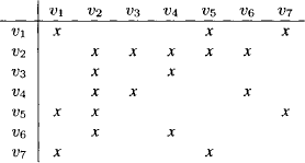
The associated graph shown in Figure 9.6 has seven nodes v1 to v7. We observe that it is already triangulated with maximal cliques {v1, v5, v7}, {v2, v5}, {v2, v3, v4} and {v2, v4, v6}. These cliques can be arranged in a join tree as shown in Figure 9.7. The node {v2, v4, v6} is chosen as root node.
Figure 9.7 The join tree of the triangulated graph in Figure 9.6.
From the left to the right in the join tree of Figure 9.7, the variables are eliminated in the following sequence: first {v1, v7}, then {v5} and {v3} until finally the variables {v2, v4, v6} in the root node remain. Hence, we may choose an elimination sequence from the set {x1, x7} × {v5} × {v3} × {v2, v4, v6}, for example (v1, v7, v5, v3, v2, v4, v6). This elimination sequence induces the following renumbering that satisfies the above requirement:
![]()
Rearranging the rows and columns of the matrix according to this numbering gives
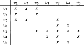
This identifies the block structure exploited in local computation. The zeros outside the blocks will not be filled-in, if the variables are eliminated in the sequence defined by the renumbering. At the end of the collect algorithm applied to the above join tree, we therefore have the following non-zero pattern of the triangular matrix:
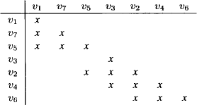
All unmarked matrix entries remain zero during the complete local computation process. Alternatively, we could also select the node {2, 5} as root and choose the elimination sequence (v1, v7, v6, v3, v4, v5, v2). This induces the renumbering:
![]()
Rearranging the rows and columns of the matrix according to this numbering gives
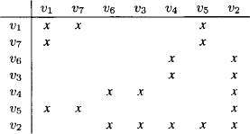
In this case, variables X1 and X7 are eliminated first and expressed by X5 in the original equations 1 and 7. Then, in the original equations 2, 4, and 6, the variable X6 is eliminated, i.e. it is expressed by X2 and X4. This process continues for the X3 and X4 until two equations for the variables X2 and X5 remain in the root node.
We obtain the following non-zero pattern of the lower triangular matrix:
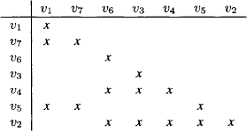
These examples show that different numberings lead to different LDLT decompositions, but the non-zero pattern represented by the join tree is always respected.
We next present an application where factorizations of symmetric, positive definite systems according to this valuation algebra occur in a natural manner.
9.2.5 An Application: The Least Squares Method
It is often the case in empirical studies that unknown parameters in a functional relationship have to be estimated from observations. Here, we assume a linear relationship between the unknown parameters. In general, there are much more observations than parameters which allows us to account for inevitable errors in the observations. This leads to overdetermined systems which cannot be solved exactly. Statistical methods are therefore needed to obtain estimates of the unknown parameters as for example the method of least squares proposed by Gauss. In this method the parameters are determined by minimizing the sum of squared residues in the linear equations. The minimization process leads to linear equations, the so-called normal equations, in the unknown parameters with a symmetric, positive definite matrix. So, the theory developed above applies. Moreover, we shall see that a decomposition of the original overdetermined systems leads to combining normal equations according to the combination rule of the valuation algebra introduced in the previous Section 9.2.1. In other words, we face here an important application of the theory developed so far.
![]() 9.1 Least Squares Method
9.1 Least Squares Method
Consider a system of linear equations
where m ≥ n, i.e. there are more equations than unknowns X1 to Xn. Also, we have introduced the residues or differences Di in order to balance the right and left-hand side of the equations. In matrix form, this system is written as AX + D = b, where A is an m × n matrix and D and b are m-vectors. We assume that the matrix A has maximal rank n. The principal idea of the least squares method is to determine the unknowns X1 to Xn such that the sum of the squares of the residues becomes minimal. This sum can be written as
![]()
So, the function to be minimized is a quadratic function of the unknowns X. For simplification we introduce the short-hand notations
![]()
where C is an n × n symmetric, positive definite matrix and c an n-vector. The sum of squares can then be written as
The necessary condition that F(X) takes a minimum is the vanishing of the gradient ∇F(X), whose i-th component can be determined from equation (9.28) as
![]()
We divide by 2 and obtain the system of equations CX − c = 0. These are the normal equations of the overdetermined system (9.27). They can also be written as
![]()
Since the matrix AT A is positive definite, the unknowns are uniquely determined by
![]()
This is the so-called least squares estimate of the unknown parameters in the system (9.27). If we compute the second order derivatives of F(X) we obtain 2C. Since C is positive definite, we conclude that the solutions of the normal equations indeed minimize the function F(X). Statistical theory justifies this way of determining the parameters, in particular, if certain probabilistic assumptions are made about the residues. We reconsider this in Chapter 10 and derive similar results by a very different method based on an isomorphic valuation algebra.
In order to solve the normal equations we may proceed as described in Section 9.2.3 and use local computation to exploit the sparsity of the normal equations. In this respect, we prove a remarkable result relating the original overdetermined system to its normal equations. In fact, already the original system may be very sparse. More precisely, we assume that we may capture this sparsity by a covering join tree for the original system. Thus, let r = {1, …, n} be the index set of the variables of the system and (V, E, λ, D) a join tree with D = P(r). We now assume that this join tree covers the system (9.27). If V = {1, …, l}, then this means that after permuting the rows of the system of equations, its matrix A decomposes into submatrices Ai for i = 1, …, l, where Ai is an mi × si matrix such that si ⊆ λ(i) and m1 + ˙ ˙ ˙ + ml = m. Therefore, every pair (Ai, bi) is covered by some node of the join tree and thus also every equation of the system (9.27). It is not excluded that some of these systems are empty, i.e. mi = 0. The following theorem claims that the corresponding normal system is decomposed into normal systems of the subsystems of the decomposition above and covered by the same join tree. Here, ⊗ denotes the combination operation of the valuation algebra of Section 9.2.1.
Theorem 9.5 Let AX + D = b be an overdetermined system and A an m × n matrix of full column rank n. Let further (V, E, λ, P(r)) be a join tree with V = {1, …, l}. If after permutation of the equations of the system AX + D = b, the matrix A decomposes into mi × si matrices Ai and b correspondingly into mi-vectors bi for i = 1, …, l, such that
1. Si ⊆ λ(i);
2. m1 + ˙ ˙ ˙ + ml = m;
3. all matrices Ai have column rank |si|;
then for C = ATA and c = ATb
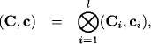
where Ci = AiT Ai and ci = AiT bi.
Proof: The proof goes by induction over the nodes of the join tree. We select node l ![]() V as a root and direct all edges towards this root. Further, we number the nodes such that i < j if node j is on the path from i to the root l. Then, node 1 is necessarily a leaf. Let s1 = s to simplify notation and
V as a root and direct all edges towards this root. Further, we number the nodes such that i < j if node j is on the path from i to the root l. Then, node 1 is necessarily a leaf. Let s1 = s to simplify notation and

If the system of equations covered by this node is empty, then we may eliminate this node directly and proceed to the next node in the numbering. Otherwise, the first m1 equations contain only variables from s. We then decompose the columns of the matrix A1 of the first m1 equations according to s − t and s ![]() t,
t,
![]()
The matrix B of the remaining m − m1 equations contains only variables from the set t. We decompose B according to s ![]() t and t into
t and t into
![]()
Then the total matrix A of the system may be decomposed into
![]()
We see that
The vector b is decomposed in the same way with respect to the first m1 and the remaining m − m1 equations:
![]()
Then, we see in the same way that
![]()
and finally conclude that
![]()
If node 1 in the join tree is eliminated, the remaining tree is still a join tree and node ch(1) is now a leaf. The remaining system of m − m1 equations with matrix B and right-hand side c can then be treated as the system above and this process may be repeated until the remaining matrix is Al and the right-hand side is bl. If t = t1 and ti for i = 2, … l − 1 denote the variables in the remaining systems obtained during this process respectively, such that tl-1 = sl, we obtain in this way
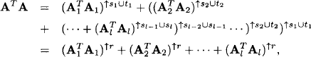
since s1 ∪ t1 = r. Similarly, we also obtain
![]()
But this means that
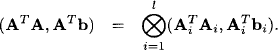
which proves the theorem.
Local computation in the valuation algebra of Section 9.2.1 is thus applicable to the least squares method for linear equations, where a factorization of the normal equation is induced by a join tree decomposition of the original overdetermined system. We shall illustrate this more concretely in the following application. Note also that if some factor in the decomposition of the original system is empty, then the induced normal system corresponds to the identity element, see Section 3.9. Finally, we refer to Chapter 10 where closely related problems are studied from a different perspective. In particular, the assumption of Theorem 9.5 that the matrix of the system has full column rank will be dropped.
![]() 9.2 Smoothing and Filtering in Linear Dynamic System
9.2 Smoothing and Filtering in Linear Dynamic System
Let X0, X1, X2 and X3 be n-dimensional variable vectors that satisfy
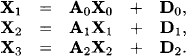
The vectors Xi may be imagined as unknown state vectors of some system, and the equations describe how these states change form time i − 1 to i, here for i ![]() {1, 2, 3}. The residues Di represent unknown disturbances which influence the development of the state over time. The matrices Ai are all regular n × n matrices. State vectors may not be observed directly, but only through some measurement devices which are described by the equations
{1, 2, 3}. The residues Di represent unknown disturbances which influence the development of the state over time. The matrices Ai are all regular n × n matrices. State vectors may not be observed directly, but only through some measurement devices which are described by the equations
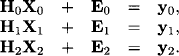
The matrices Hi are m × n matrices and the vectors yi, representing observed values, give information about the unknown states. The residues Ei again represent unknown measurement errors. The task is to estimate the values of the state vectors from these equations and the observations. We first bring the equations into the form of system (9.27):
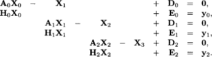
We observe that the system can be decomposed into three subsystems, each consisting of two consecutive equations that are covered by the three nodes of the simple join tree in Figure 9.8. In order to apply Theorem 9.5, we assume that the subsystems have full column rank, i.e. that m ≥ n, and that Hi have full column rank too. If we switch to the valuation algebra of symmetric, positive definite systems, then by Theorem 9.5 the normal equations of the total system can be decomposed into
Figure 9.8 The join tree covering the equations of the linear dynamic system.

![]()
where
![]()
and
![]()
for i ![]() {0, 1, 2}. This allows us to apply local computation for the solution of the normal equations using the collect algorithm as described in Section 9.2.2 or the fusion algorithm. If we select the rightmost node in Figure 9.8 as the root, we eliminate first X0 and then X1 i.e. we express X0 in terms of X1 and then X1 in terms of X2. The variables X2 are eliminated in the last node to obtain X3. Determining the last state, given the past and present measurements is called a filter solution. Then, by backward substituting, the least squares estimates of the other states can be computed. This is called the smoothing solution.
{0, 1, 2}. This allows us to apply local computation for the solution of the normal equations using the collect algorithm as described in Section 9.2.2 or the fusion algorithm. If we select the rightmost node in Figure 9.8 as the root, we eliminate first X0 and then X1 i.e. we express X0 in terms of X1 and then X1 in terms of X2. The variables X2 are eliminated in the last node to obtain X3. Determining the last state, given the past and present measurements is called a filter solution. Then, by backward substituting, the least squares estimates of the other states can be computed. This is called the smoothing solution.
We examine this procedure a bit more closely. In terms of message-passing, the message from the leftmost node X0, X1 in the join tree of Figure 9.8 corresponds to the elimination of X0. The message is the projection of (C0, c0) to the variables X1 which, according to (9.13) and (9.14), is
![]()
where
![]()
This matrix is the sum of two positive definite matrices and is thus positive definite itself, i.e. it has an inverse. The elimination process for X0 in the first subsystem leads to the equation
![]()
which can later be used for backward substitution, once X1 is determined. Passing the message to the next node of the join tree and combining it to the node content is equivalent to substituting this expression for X0 in the second subsystem. More generally, let us define for i = 0, 1, 2, …
![]()
and
![]()
where ∑-1,0 = 0 and v-1,0 = y0. Since combination (9.15) corresponds to matrix addition, the system on the node Xi, Xi+1 at step i of the collect algorithm is:
![]()
Due to (9.13) and (9.14), the message from node Xi-1, Xi to node Xi, Xi+1 computed by eliminating Xi-1 is
![]()
for i = 1, 2, … and the eliminated variables in this step can be expressed as
![]()
If the sequence stops with X3 as in our example, then eliminating X2 in the subsystem on the middle node in join tree of Figure 9.8 gives
![]()
hence
![]()
This is also called a one-step predictor for X3 and can be used to start backward substitution: first for X2, then for X1 and finally for X0. Such linear dynamic systems will be reconsidered from a more general point of view in Section 10.5. In particular, it will be shown that the assumption that Hi has full column rank can be dropped. This closes our discussion of ordinary linear systems and we next focus on linear fixpoint equation systems. A third class of linear systems called linear systems with Gaussian disturbances will be studied in Section 10.1.
9.3 SEMIRING FIXPOINT EQUATION SYSTEMS
A linear fixpoint equation system takes the form MX + b = X, where M is an n × n matrix, X an n-vector of variables and b an n-vector. If the matrix M and the vector b take values from a field, we may express the fixpoint system as (I − M)X = b and by defining A = I − M we obtain an ordinary linear system AX = b. This allows us to apply the theory of the previous sections and shows that fixpoint equation systems over fields do not need to be considered separately. However, we pointed out in Section 6.2 that the computation of path problems amounts to the solution of fixpoint equation systems over semirings. Moreover, we identified a particular class of semirings called quasi-regular semirings, where all fixpoint equations provide a solution determined by the star operation. If ![]() A, +, x, *, 0, 1
A, +, x, *, 0, 1![]() denotes a quasi-regular semiring, then the set M(A, n) of n × n matrices with values from A also forms a quasi-regular semiring with the inductive definition of the star operation given in equation (6.17), see Theorem 6.2. Hence, a solution to the fixpoint equation MX + b = X in a quasi-regular semiring is always given by the element M*b. How is this related to fixpoint equations over real numbers and thus to ordinary equation systems? It was shown in Example 6.11 that real numbers
denotes a quasi-regular semiring, then the set M(A, n) of n × n matrices with values from A also forms a quasi-regular semiring with the inductive definition of the star operation given in equation (6.17), see Theorem 6.2. Hence, a solution to the fixpoint equation MX + b = X in a quasi-regular semiring is always given by the element M*b. How is this related to fixpoint equations over real numbers and thus to ordinary equation systems? It was shown in Example 6.11 that real numbers ![]() ∪ {∞} form a quasi-regular semiring with the definition
∪ {∞} form a quasi-regular semiring with the definition
![]()
for a ≠ 1 and a* = ∞ for a = 1. If we now consider its induced semiring of matrices and further assume that I − M is regular, then the fixpoint system MX + b = X has a unique solution that must be equal to the result of the star operation,
![]()
By applying the star operation to I − M we obtain
![]()
which solves the regular system MX = b. On the other hand, if we directly compute (I − M)* without caring about the regularity of I − M, then the result corresponds to the inverse matrix of M, if (I − M)* does not contain the adjoined semiring element ∞. This follows from Theorem 6.18 and the uniqueness of the inverse matrix (Lehmann, 1976). Concluding, we see that fixpoint equation systems over quasi-regular semirings indeed provide an important generalization of ordinary linear systems. Semiring fixpoint equations induce two different types of valuation algebras which will both be used in the remaining parts of this chapter to obtain a local computation based solution to such equations. First, we focus on quasi-regular valuation algebras from Section 6.4 which leads to a solution approach that is similar to local computation with symmetric, positive definite systems studied in Section 9.2.2. The second approach is based on Kleene valuation algebras from Section 6.7 and leads to an interesting compilation approach which is based on the query answering technique for idempotent valuation algebras in Section 4.6. However, computation in both valuation algebras requires evaluating the star operation for matrices over quasi-regular semirings. The following section therefore presents first a well-known algorithm for this task.
9.3.1 Computing Quasi-Inverse Matrices
For a finite index set s, the set of labeled matrices M(A, s) with values from a quasi-regular semiring ![]() A, +, x, *, 0, 1
A, +, x, *, 0, 1![]() forms itself a quasi-regular semiring with the inductive definition of the star operation given in equation (6.17). This operation is performed as part of the projection rule in quasi-regular valuation algebras, respectively as part of the combination rule in Kleene valuation algebras. In the latter case, we often use the alternative induction of equation (6.31), but it has also been shown that the two definitions are equivalent for Kleene algebras. It is therefore sufficient for both algebras to dispose of an algorithm that computes a quasi-inverse matrix M* for M
forms itself a quasi-regular semiring with the inductive definition of the star operation given in equation (6.17). This operation is performed as part of the projection rule in quasi-regular valuation algebras, respectively as part of the combination rule in Kleene valuation algebras. In the latter case, we often use the alternative induction of equation (6.31), but it has also been shown that the two definitions are equivalent for Kleene algebras. It is therefore sufficient for both algebras to dispose of an algorithm that computes a quasi-inverse matrix M* for M ![]() M(A, s) that satisfies the fixpoint equation
M(A, s) that satisfies the fixpoint equation
The well-known Warshall-Floyd-Kleene algorithm proposed by (Roy, 1959; Warshall, 1962; Floyd, 1962; Kleene, 1956) computes quasi-inverses iteratively by the following formula: For s = {1, …, n} and k = 0, …, n we define
with M(0) = M. Note that the operation of matrix projection is used to refer to the k-th column and row of the matrix M. Also, we again omit the explicit writing of the semiring multiplication symbol. It is proved in (Lehmann, 1976) that M(n) + I indeed corresponds to the quasi-inverse of equation (6.17), which implies that
![]()
satisfies equation (9.29) as a consequence of Theorem 6.2. Formula (9.30) therefore provides a general algorithm for the computation of the star operation in M(A, s) using only the semiring operations in A. The space complexity of this algorithm is ![]() (|s|2) because it only needs to store two matrices. Given two indices i,j
(|s|2) because it only needs to store two matrices. Given two indices i,j ![]() s, equation (9.30) is equivalently expressed as
s, equation (9.30) is equivalently expressed as
![]()
This shows that an implementation required three nested loops for the indices i,j and k, which leads to a time complexity of ![]() (|s|3). It is important to note that the theory in the subsequent sections is independent on the actual algorithm used to compute the star operation of matrices over quasi-regular semirings and Kleene algebras. Here, we presented the Warshall-Floyd-Kleene algorithm but there are other algorithms as for example the Gauss-Jordan method. However, we will use the Warshall-Floyd-Kleene algorithm to reason about the complexity of local computation based approaches to the solution of semiring fixpoint equation systems, but if another algorithm is present for some particular quasi-regular semirings that outperforms the Warshall-Floyd-Kleene algorithm or its implementation, then this algorithm can be used and its gain in efficiency also carries over to the local computation scheme.
(|s|3). It is important to note that the theory in the subsequent sections is independent on the actual algorithm used to compute the star operation of matrices over quasi-regular semirings and Kleene algebras. Here, we presented the Warshall-Floyd-Kleene algorithm but there are other algorithms as for example the Gauss-Jordan method. However, we will use the Warshall-Floyd-Kleene algorithm to reason about the complexity of local computation based approaches to the solution of semiring fixpoint equation systems, but if another algorithm is present for some particular quasi-regular semirings that outperforms the Warshall-Floyd-Kleene algorithm or its implementation, then this algorithm can be used and its gain in efficiency also carries over to the local computation scheme.
Algorithm 9.1 The Warshall-FIoyd-Kleene Algorithm
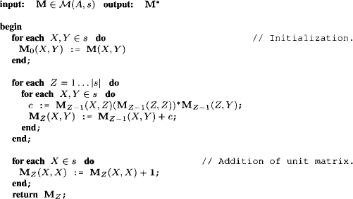
9.3.2 Local Computation with Quasi-Regular Valuations
We focus in this section on a local computation based solution of fixpoint equation systems X = MX + b defined over a quasi-regular semiring ![]() A, +, x, *, 0, 1
A, +, x, *, 0, 1![]() . For variables X1, …, Xn and the associated index set r = {1, …, n}, we assume for s ⊆ r that M
. For variables X1, …, Xn and the associated index set r = {1, …, n}, we assume for s ⊆ r that M ![]() M(A, s) is an s × s matrix of semiring values, X an s-vector of variables and b an s-vector of semiring values. It was shown in Section 6.4 that such systems correspond to valuations
M(A, s) is an s × s matrix of semiring values, X an s-vector of variables and b an s-vector of semiring values. It was shown in Section 6.4 that such systems correspond to valuations ![]() = (A, b) with domain d(
= (A, b) with domain d(![]() ) = s in the quasi-regular valuation algebra
) = s in the quasi-regular valuation algebra ![]() Φ, D
Φ, D![]() induced by the semiring A, where D = P(r). We observe the similar structure with the valuation algebra of symmetric, positive definite systems in Section 9.2.1: in both algebras, valuations are pairs of square matrices and vectors, the operations of combination defined in the equations (6.30) and (9.15) are identical, and also the operations of projection given in the equations (6.23) and (9.14) look very similar.
induced by the semiring A, where D = P(r). We observe the similar structure with the valuation algebra of symmetric, positive definite systems in Section 9.2.1: in both algebras, valuations are pairs of square matrices and vectors, the operations of combination defined in the equations (6.30) and (9.15) are identical, and also the operations of projection given in the equations (6.23) and (9.14) look very similar.
As usual for local computation, we subsequently assume that ![]() = (M, b) is given as a factorization or decomposition
= (M, b) is given as a factorization or decomposition ![]() =
= ![]() 1 ⊗ … ⊗
1 ⊗ … ⊗ ![]() m of quasi-regular valuations
m of quasi-regular valuations ![]() i = (Mi, bi)
i = (Mi, bi) ![]() Φ with i = 1, …, m. It is important to note that the following local computation based solution solves any such factorized system. But since we motivated semiring fixpoint equations from the perspective of the algebraic path problem in Chapter 6, we subsequently go into this important application field. Moreover, when the system (M, b) models a path problem in a graph, such factorizations often come from the underlying graph. Imagine, for example, that we want to compute shortest distances between cities of different European countries from road maps that contain only direct distances between neighboring cities, see Instance 6.2. Hence, let s denote the set of all European cities. Instead of a single road map M that contains all cities of Europe, it is more natural to consider local maps Mi for each country with some overlapping region to neighboring countries. Since matrix addition corresponds to minimization in the tropical semiring, we clearly have
Φ with i = 1, …, m. It is important to note that the following local computation based solution solves any such factorized system. But since we motivated semiring fixpoint equations from the perspective of the algebraic path problem in Chapter 6, we subsequently go into this important application field. Moreover, when the system (M, b) models a path problem in a graph, such factorizations often come from the underlying graph. Imagine, for example, that we want to compute shortest distances between cities of different European countries from road maps that contain only direct distances between neighboring cities, see Instance 6.2. Hence, let s denote the set of all European cities. Instead of a single road map M that contains all cities of Europe, it is more natural to consider local maps Mi for each country with some overlapping region to neighboring countries. Since matrix addition corresponds to minimization in the tropical semiring, we clearly have
Further, we explained at the very end of Section 6.3 that the vector b serves to specify the distances to be computed. If we are interested in the shortest distances between all possible cities of Europe and a selected target city T ![]() s, we define the vector b such that b(T) = 1 and b(Y) = 0 for all Y
s, we define the vector b such that b(T) = 1 and b(Y) = 0 for all Y ![]() s − {T}. Solving the fixpoint equation X = MX + b then corresponds to the single-target shortest distance problem and its transposed system represents the single-source problem. The vectors bi are therefore specified with respect to query and must satisfy
s − {T}. Solving the fixpoint equation X = MX + b then corresponds to the single-target shortest distance problem and its transposed system represents the single-source problem. The vectors bi are therefore specified with respect to query and must satisfy
![]()
This gives us a natural factorization
![]()
for the shortest distance problem. If x = M*b is a solution to the system (M, b), it contains the shortest distances between all European cities and the selected target city T ![]() s. For an arbitrary source city S
s. For an arbitrary source city S ![]() s, it follows from Theorem 6.3 that
s, it follows from Theorem 6.3 that
![]()
Hence, the single-pair problem requires to compute
![]()
and we therefore obtain its solution by solving the single-query inference problem
![]()
This can either be done by the fusion or collect algorithm. As for symmetric, positive definite systems in Section 9.2.2, we finally compute the complete solution x by a step-wise extension of the single-pair solution in a solution construction process. To do so, we show in this section that solutions to quasi-regular fixpoint equations satisfy the requirements for general solutions in valuation algebras imposed in Section 8.1. This allows us to directly apply one of the generic solution construction procedures.
Alternatively, if no natural factorization of the sparse system ![]() = (M, b) exists, we have to produce a decomposition
= (M, b) exists, we have to produce a decomposition ![]() =
= ![]() 1 ⊗ … ⊗
1 ⊗ … ⊗ ![]() m. There are many applications of path problems where the adjacency matrix is symmetric. Imagine for example the modelling of air-line distances, which are always symmetric. We then obtain a decomposition by applying the graphical theory of Section 9.2.4. This follows from the similar structure between the two valuation algebras mentioned above. On the other hand, if the matrix is not symmetric, then the construction of the graph for the triangulation process must be modified. We propose this as Exercise 1.1 to the reader. By application of local computation, we exploit the sparsity in the system
m. There are many applications of path problems where the adjacency matrix is symmetric. Imagine for example the modelling of air-line distances, which are always symmetric. We then obtain a decomposition by applying the graphical theory of Section 9.2.4. This follows from the similar structure between the two valuation algebras mentioned above. On the other hand, if the matrix is not symmetric, then the construction of the graph for the triangulation process must be modified. We propose this as Exercise 1.1 to the reader. By application of local computation, we exploit the sparsity in the system ![]() = (M, b) captured by the factorization or decomposition. As shown below, this is again similar to local computation for symmetric, positive definite systems studied in Section 9.2.2 and also follows the same principle of locality.
= (M, b) captured by the factorization or decomposition. As shown below, this is again similar to local computation for symmetric, positive definite systems studied in Section 9.2.2 and also follows the same principle of locality.
We now propose a suitable definition of configuration extension sets for quasi-regular valuation algebras: for ![]() = (M, b)
= (M, b) ![]() Φ with d(
Φ with d(![]() ) = s and t ⊆ s we define the configuration extension set for an arbitrary t-vector x to
) = s and t ⊆ s we define the configuration extension set for an arbitrary t-vector x to ![]() as
as
(9.32) ![]()
Again, observe the similarity to the definition of configuration extension sets for symmetric, positive definite systems in equation (9.19). The following theorem shows that this definition also satisfies the requirements for general solution extension sets in valuation algebras imposed in Section 8.1.
Theorem 9.6 Solution extension sets in quasi-regular valuation algebras satisfy the property of Definition 8.1, i.e. for all ![]()
![]() Φ with t ⊆ u ⊆ s = d(
Φ with t ⊆ u ⊆ s = d(![]() ) and all t-vectors x we have
) and all t-vectors x we have
![]()
Proof: For an arbitrary t-vector x let
![]()
It then follows from Lemma 6.2 and Definition 6.4 that y is the solution to the system
![]()
We therefore have
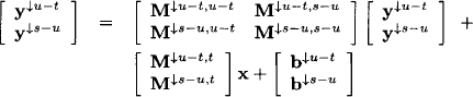
and obtain the two systems
![]()
From the second equation follows that y↓s-u is the solution to
![]()
We must therefore have
We insert this expression into the first equation and obtain after rearranging terms:
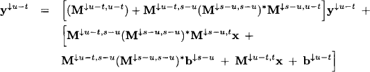
Next, we observe the following identities:
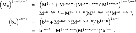
This follows from the definition of projection in the equations (6.24) and (6.25). Likewise, we also have
![]()
We insert these identities in equation (9.34) and obtain
![]()
We observe that y↓u-t is the solution to the system
![]()
and it must again hold that
![]()
This shows that y↓u-t ![]()
![]() (x). Finally, we conclude from equation (9.33)
(x). Finally, we conclude from equation (9.33)
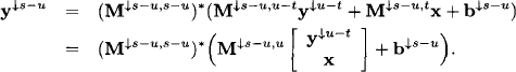
This implies that y↓s-u ![]() W
W![]() u(y↓u-t, x).
u(y↓u-t, x).
Configuration extension sets therefore fulfill the requirements for the generic solution construction procedure of Section 8.2.1, that builds the solution set
(9.35) ![]()
based on the results of a multi-query local computation procedure. However, remember that the combination rule for quasi-regular valuation algebras and symmetric, positive definite systems are identical, see equations (6.30) and (9.15). For symmetric, positive definite systems we know from Lemma 9.3 that they also satisfy the additional condition of Theorem 8.3 for solution construction based on the results of a single-query architecture. This property is only based on the combination operator and therefore also holds for quasi-regular valuation algebras.
Lemma 9.4 Quasi-regular valuation algebras satisfy the property that for all ψ1, ψ2 ![]() Φ with d(ψ1) = s, d(ψ2) = t, s ⊆ u ⊆ s ∪ t and u-vector x we have
Φ with d(ψ1) = s, d(ψ2) = t, s ⊆ u ⊆ s ∪ t and u-vector x we have
![]()
Hence, we can conclude from Section 8.2.3 that Algorithm 8.4 returns the solution to a factorized, quasi-regular fixpoint equation system based on the results of a single-query local computation architecture. The actual process is very similar to the case of symmetric, positive definite systems, which we considered in detail in Section 9.2.2.
To determine the complexity of solving fixpoint equation systems by local computation, we first remind that projection is the more time consuming operation than combination. For ![]() = (M, b)
= (M, b) ![]() Φ with d(
Φ with d(![]() ) = s and t ⊆ s, the projection rule for quasi-regular valuations, given in equation (6.23), is
) = s and t ⊆ s, the projection rule for quasi-regular valuations, given in equation (6.23), is
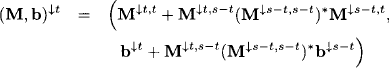
includes the evaluation of the star operation for matrices and this has a cubic time complexity in the general case, as shown in Section 9.3.1. However, let us now rewrite this operation with variable elimination instead of projection. If t = s − {Z} for some Z ![]() s, the matrix component of this operation becomes
s, the matrix component of this operation becomes
![]()
which requires computing
![]()
for all X, Y ![]() s − {Z}. This expression does not apply the star operation to matrices anymore. Since the same holds for the vector component, the operation of variable elimination adopts a quadratic time complexity. This motivates the application of the fusion algorithm instead of collect. Moreover, the size of the valuation stored in a join tree node is bounded by the treewidth ω* which then also gives an upper bound for the time complexity of the operations of combination and variable elimination. To sum it up, the time and space complexity of applying the fusion algorithm to quasi-regular valuations is
s − {Z}. This expression does not apply the star operation to matrices anymore. Since the same holds for the vector component, the operation of variable elimination adopts a quadratic time complexity. This motivates the application of the fusion algorithm instead of collect. Moreover, the size of the valuation stored in a join tree node is bounded by the treewidth ω* which then also gives an upper bound for the time complexity of the operations of combination and variable elimination. To sum it up, the time and space complexity of applying the fusion algorithm to quasi-regular valuations is
![]()
The single-target path problem with target node T ![]() s is represented by the fixpoint equation X = MX + bT with b(T) = 1 and b(Y) = 0 for all Y
s is represented by the fixpoint equation X = MX + bT with b(T) = 1 and b(Y) = 0 for all Y ![]() s − {T}. Its solution x = M*hT corresponds to the column of the matrix M* that corresponds to the variable T. If we solve this problem for all possible target nodes, we completely determine the matrix M* and thus solve the all-pairs path problem. This is possible with |s| repetitions of the above local computation procedure using the same matrix M but different vectors. In other words, we have a prototype application for a compilation approach such as the LDR-decomposition for regular systems in Section 9.1.4 or the LDLT-decomposition for symmetric, positive definite systems in Section 9.2.3. In fact, it was shown by (Backhouse & Carré, 1975) that LDR-decomposition can also be applied to regular algebras, which are quasi-regular semirings with idempotent addition. This approach was later generalized by (Radhakrishnan et al., 1992) to quasi-regular semirings. We propose the development of LDR-decomposition for matrices with values from a quasi-regular semiring as Exercise 1.2 to the reader. In the following section, we focus on an alternative approach based on Kleene valuation algebras that computes some selected values of the quasi-inverse matrix M* directly. This corresponds to the multiple-pairs algebraic path problem which does not assume specific source or target nodes.
s − {T}. Its solution x = M*hT corresponds to the column of the matrix M* that corresponds to the variable T. If we solve this problem for all possible target nodes, we completely determine the matrix M* and thus solve the all-pairs path problem. This is possible with |s| repetitions of the above local computation procedure using the same matrix M but different vectors. In other words, we have a prototype application for a compilation approach such as the LDR-decomposition for regular systems in Section 9.1.4 or the LDLT-decomposition for symmetric, positive definite systems in Section 9.2.3. In fact, it was shown by (Backhouse & Carré, 1975) that LDR-decomposition can also be applied to regular algebras, which are quasi-regular semirings with idempotent addition. This approach was later generalized by (Radhakrishnan et al., 1992) to quasi-regular semirings. We propose the development of LDR-decomposition for matrices with values from a quasi-regular semiring as Exercise 1.2 to the reader. In the following section, we focus on an alternative approach based on Kleene valuation algebras that computes some selected values of the quasi-inverse matrix M* directly. This corresponds to the multiple-pairs algebraic path problem which does not assume specific source or target nodes.
9.3.3 Local Computation with Kleene Valuations
For an index set r = {1, …, n} and s ⊆ r, the solution to the all-pairs algebraic path problem M* defined by the matrix M ⊆ M(A, s) is a solution to the fixpoint system X = MX + I. Here, X is an s × s matrix of variables, M an s × s matrix of semiring values and I the unit matrix in M(A, s). We further assume in this section that the semiring ![]() A, +, x, *, 0, 1
A, +, x, *, 0, 1![]() is a Kleene algebra according to Definition 6.6. It then follows from Theorem 6.5 that the set of labeled matrices M(A, s) also forms a Kleene algebra, and we obtain its induced Kleene valuation algebra
is a Kleene algebra according to Definition 6.6. It then follows from Theorem 6.5 that the set of labeled matrices M(A, s) also forms a Kleene algebra, and we obtain its induced Kleene valuation algebra ![]() Φ, D
Φ, D![]() by defining D = P(r) and
by defining D = P(r) and
![]()
as shown in Theorem 6.6. Consequently, we may consider the solution M* to the all-pairs path problem over a Kleene algebra as an element of a valuation algebra. With regard to inference problems, we declare this element as the objective function and assume a knowledgebase {M1*, …, Mn*} ⊆ Φ such that
![]()
This corresponds to the situation of having an existing factorization for the path problem solution. Alternatively, we could take a factorization of the original matrix M and start from a set of matrices {M1, …, Mm} with Mi ![]() M(A, si) and si ⊆ s for i = 1, …, m such that
M(A, si) and si ⊆ s for i = 1, …, m such that
This second factorization represents in the example of the previous section the local road maps for each country, whereas the elements of the first factorization correspond to tables of shortest distances that already exist for each country. Although probably more realistic, the second factorization cannot be considered as a knowledgebase directly, because the factors Mi are generally not contained in Φ. But as this example foreshadows, it proves sufficient to compute the closure of each factor in order to obtain a knowledgebase that factors M* as a consequence of Lemma 6.11 and 6.17:
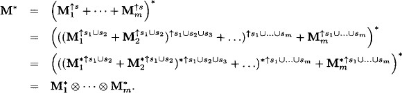
The last equality follows from the definition of combination in Kleene valuation algebras given in equation (6.38). Thus, we may either start from a factorization of the path problem solution, which directly gives a knowledgebase of Kleene valuations, or produce the latter from a factorization of the path problem input matrix. Note that the second case includes the type of factorization that was considered for quasi-regular valuation algebras in equation (9.31). Alternatively, if no natural factorization of either the closure or the input matrix exists, we may exploit the idempotency of semiring addition to produce a decomposition of the matrix M ![]() M(A, s) that satisfies equation (9.36): For X, Y
M(A, s) that satisfies equation (9.36): For X, Y ![]() s and X ≠ Y,
s and X ≠ Y,
- if M(X, Y) ≠ 0 or M(F, X) ≠ 0, add M↓{X, Y} to the factorization;
- if M(X, X) ≠ 0, add M↓{X} to the factorization.
This creates a factorization of minimal granularity where the domain of each factor contains at most two variables. Note also that the same diagonal value M(X, X) possibly occurs in multiple factors. This, however, does not matter as a consequence of idempotent semiring addition in a Kleene algebra. Moreover, if the Kleene algebra is a bounded semiring with the property a + 1 = 1 for all a ![]() A, it follows from equation (9.29) that M*(X, X) = 1 for all X
A, it follows from equation (9.29) that M*(X, X) = 1 for all X ![]() s and independently of the original values of M(X, X). In this case, we can ignore the diagonal elements in the decomposition process. Also, the semantics of path problems often yield input matrices where most of the diagonal elements are M(X, X) = 1. Then, the decomposition process also leads to factors that share this property, and the following lemma shows that these factors are equal to their closures. This simplifies the process of building a knowledgebase from the decomposition process considerably, as illustrated in Example 9.5.
s and independently of the original values of M(X, X). In this case, we can ignore the diagonal elements in the decomposition process. Also, the semantics of path problems often yield input matrices where most of the diagonal elements are M(X, X) = 1. Then, the decomposition process also leads to factors that share this property, and the following lemma shows that these factors are equal to their closures. This simplifies the process of building a knowledgebase from the decomposition process considerably, as illustrated in Example 9.5.
Lemma 9.5 In a bounded Kleene algebra we have
(9.37) ![]()
Proof: We apply equation (6.32) and remark that the property of boundedness implies f = b + ce* d = 1. It follows from Property (KP3) in Lemma 6.8 that f = f* = 1, and the statement then follows directly.
Example 9.5 Consider the variable set s = {Berlin, Paris, Rome, Berne} and the following sparse matrix defined over the tropical semiring of non-negative integers ![]()
![]() ∪ {0, ∞}, min, +, ∞, 0
∪ {0, ∞}, min, +, ∞, 0![]() expressing the path lengths between some selected cities:
expressing the path lengths between some selected cities:
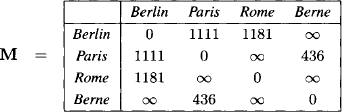
This table might be seen as the direct distances in a road map, where the symbol ∞ tags unknown distances or the absence of a direct connection in the road map. The matrix M then factorizes as
![]()
with factors
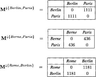
We further recall from Example 5.10 that the tropical semiring is bounded with the integer 0 as unit element. By Lemma 9.5 the above factors are equal to their closures and therefore directly form a knowledgebase, i.e. a factorization of the yet unknown solution M*. We have
![]()
The second component of an inference problem is the query set. When solving the multiple-pairs path problem, we are interested in the semiring values M*(X, Y) for certain pairs of variables (X, Y) from the domain s = d(M*) of the objective function. To extract these values, it is in fact not necessary to compute the objective function M* completely, but only the marginals M*↓{X,Y} must be available. The queries of the inference problem are therefore given by sets of variables {X, Y} for non-diagonal entries and {X} for the diagonal entries of the objective function. Depending on the structure of the query set, we retrieve the classical types of path problems: when the query set consists of a single element {X, Y}, the inference problem corresponds to a single-pair algebraic path problem. If the query set if formed by all possible pairs of variables {X, Y}, we solve the all-pairs algebraic-path problem. If for a selected variable X ![]() s, the query set contains the pairs {X, Y} for all nodes Y
s, the query set contains the pairs {X, Y} for all nodes Y ![]() s with X ≠ Y, we find the single-source algebraic path problem. Note that since we consider sets of variables, this is equivalent to the single-target algebraic path problem. Finally, if the non-empty query set has no such structure, we refer to the inference problem as the multiple-pairs algebraic path problem. It will later be shown in this section that we can completely pass on the explicit definition of query sets when dealing with Kleene valuation algebras. This, however, requires some complexity considerations with respect to the local computation process. Until then, we assume such an explicit query set as part of the inference problem and next focus on the local computation based solution process.
s with X ≠ Y, we find the single-source algebraic path problem. Note that since we consider sets of variables, this is equivalent to the single-target algebraic path problem. Finally, if the non-empty query set has no such structure, we refer to the inference problem as the multiple-pairs algebraic path problem. It will later be shown in this section that we can completely pass on the explicit definition of query sets when dealing with Kleene valuation algebras. This, however, requires some complexity considerations with respect to the local computation process. Until then, we assume such an explicit query set as part of the inference problem and next focus on the local computation based solution process.
Given an inference problem with a knowledgebase of Kleene valuations and a query set, its solution can be delegated to one of the generic local computation methods introduced in Chapter 4. Since Kleene valuation algebras are idempotent, we go for the particularly simple idempotent architecture of Section 4.5. We first construct a join tree (V, E, λ, D) that covers the inference problem according to Definition 3.8 and execute the chosen architecture. At then end of the message-passing, each join tree node i ![]() V contains M*↓λ(i) as a consequence of Theorem 4.4. The result of each query {X, Y} is finally obtained by finding a covering node i
V contains M*↓λ(i) as a consequence of Theorem 4.4. The result of each query {X, Y} is finally obtained by finding a covering node i ![]() V with {X, Y}
V with {X, Y} ![]() λ(i) and performing one last projection per query
λ(i) and performing one last projection per query
This shows how local computation solves multiple-pairs path problems represented as inference problems over Kleene valuation algebras. Let us next consider the complexity of this approach in more detail: since Kleene valuations are labeled matrices, the space requirement to store a valuation M* with domain d(M*) = s is ![]() (|s|2). Concerning the time complexity of the valuation algebra operations, we first remark that combination is the more expensive operation. Projection only drops rows and columns, whereas the combination of two Kleene valuations M1* and M2* with domains d(M1*) = s and d(M2*) = t performs a component-wise addition of the two matrices and computes the closure of the result. Applying the Warshall-Floyd-Kleene algorithm of Section 9.3.1 therefore gives a time-complexity of
(|s|2). Concerning the time complexity of the valuation algebra operations, we first remark that combination is the more expensive operation. Projection only drops rows and columns, whereas the combination of two Kleene valuations M1* and M2* with domains d(M1*) = s and d(M2*) = t performs a component-wise addition of the two matrices and computes the closure of the result. Applying the Warshall-Floyd-Kleene algorithm of Section 9.3.1 therefore gives a time-complexity of ![]() (|s ∪ t|3) for the operation of combination. Based on the time and space complexity of Kleene valuations and the generic complexity analysis for the idempotent architecture in Section 4.5.1, we conclude that the message-passing process adopts a total time and space complexity of
(|s ∪ t|3) for the operation of combination. Based on the time and space complexity of Kleene valuations and the generic complexity analysis for the idempotent architecture in Section 4.5.1, we conclude that the message-passing process adopts a total time and space complexity of
where ω* denotes the treewidth of the inference problem and |V| the number of join tree nodes. This may be compared with a direct computation of M* that adopts a time and space complexity of ![]() (|s|3) and
(|s|3) and ![]() (|s|2) respectively. Since it is always possible to apply the fusion and bucket elimination algorithms to knowledgebases of Kleene valuations, we may assume that |V| ≈ |s| when comparing the two approaches. Depending on the treewidth and thus on the sparsity of the input matrix, the difference to the local computation complexity of equation (9.39) may be considerable, as shown in the following example.
(|s|2) respectively. Since it is always possible to apply the fusion and bucket elimination algorithms to knowledgebases of Kleene valuations, we may assume that |V| ≈ |s| when comparing the two approaches. Depending on the treewidth and thus on the sparsity of the input matrix, the difference to the local computation complexity of equation (9.39) may be considerable, as shown in the following example.
Example 9.6 Assume that we are charged with the task of computing the travelling distances of packets for a European express delivery service. Two different rules apply for national and international shipping: In order to guarantee fast delivery, packets are transported from the source to the target city directly, if both cities are in the same country. Otherwise, packets are first transported to an international distribution center. For simplicity, we assume that only one distribution center exists per country. If we for example send a packet from a Portuguese city to a French city, the packet is first transported to the Portuguese distribution center, then to the Spanish distribution center, then to the French distribution center and finally to the French address. It is furthermore assumed that the delivery service always chooses the shortest travelling distance and that packets are transported by car or train. The data of this example consists of a local map for each country including its distribution center and the 99 largest cities and villages. Hence, if we include 43 European countries with a common land frontier to another European country, we have |s| = 4300. In addition, the local road maps contain only the direct distances between neighboring cities and villages in the corresponding country and the direct distances between its own distribution center and the distribution centers of all neighboring countries with a common land frontier. If we model these maps as valuations over the tropical semiring of non-negative integers, we obtain a knowledgebase of 43 valuations. The 9 neighboring countries of Germany are never exceeded in our example, which implies that the German map contains exactly 9 international distances. The largest domain of all valuations in the knowledgebase is therefore 109. Let us compare different approaches for the computation of the required distances. First, we could unify all local road maps to a single European road map and compute its closure. The complexity of ![]() (|s|3) for computing closures by the Warshall-Floyd-Kleene algorithm gives us an estimation of 43003 = 79’507’000’000 operations for this approach. A more intelligent way of solving this problem exploits the observation that it is in fact sufficient to know all shortest distances between the distribution centers. An international distance between two cities can then be computed by adding the shortest distances to their corresponding distribution centers and the distance between the two distribution centers. Hence, we create a European road map that contains only the distribution centers and compute its closure together with the closures of all local road maps for the national distances. Since the largest map has 109 cities, the computational effort of this approach is bounded by (43 + 1) ˙ 1093 = 56’981’276 operations. This is a very rough estimation such that we can ignore the two additions needed to obtain an international distance. We observe that the second approach is more efficient because it exploits the problem structure. Finally, we could solve this problem by local computation. The OSLA-SC algorithm of Section 3.7 implemented in the NENOK framework (Pouly, 2010) returns a join tree with a treewidth of ω* + 1 = 109. This shows that the join tree identifies the same problem structure and local computation essentially mirrors the computations of the second approach.
(|s|3) for computing closures by the Warshall-Floyd-Kleene algorithm gives us an estimation of 43003 = 79’507’000’000 operations for this approach. A more intelligent way of solving this problem exploits the observation that it is in fact sufficient to know all shortest distances between the distribution centers. An international distance between two cities can then be computed by adding the shortest distances to their corresponding distribution centers and the distance between the two distribution centers. Hence, we create a European road map that contains only the distribution centers and compute its closure together with the closures of all local road maps for the national distances. Since the largest map has 109 cities, the computational effort of this approach is bounded by (43 + 1) ˙ 1093 = 56’981’276 operations. This is a very rough estimation such that we can ignore the two additions needed to obtain an international distance. We observe that the second approach is more efficient because it exploits the problem structure. Finally, we could solve this problem by local computation. The OSLA-SC algorithm of Section 3.7 implemented in the NENOK framework (Pouly, 2010) returns a join tree with a treewidth of ω* + 1 = 109. This shows that the join tree identifies the same problem structure and local computation essentially mirrors the computations of the second approach.
The complexity of solving a path problem by local computation depends on the treewidth of the inference problem, which also includes the query set. Query answering according to equation (9.38) presupposes that for each query {X, Y}, it is possible to find some join tree node i ![]() V that covers this query. This important aspect was ignored in Example 9.6. The join tree must therefore ensure that each query is covered by some node, and this blows up the node labels. In other words, the larger the query set is, the larger becomes the treewidth of the inference problem, and the less efficient is local computation. The worst-case scenario is the all-pairs algebraic path problem where the query set is built from all possible pairs of variables. Every covering join tree for such an inference problem contains at least one node whose label equals the domain of the objective function. We thus have ω* + 1 = |s| and the message-passing process essentially mirrors the direct computation of the objective function. Conversely, if the query set is empty (or if each query is covered by some knowledgebase factor), the treewidth depends only on the sparsity of the matrix, which results in the best possible performance of local computation. From this point of view, the query set may destroy the gain of the sparsity in the knowledgebase. However, there are two properties of Kleene valuation algebras that allow us to ignore the query set and benefit from a treewidth that only depends on the knowledgebase. These are the polynomial complexity of Kleene valuations and the property of idem-potency. Section 4.6 and in particular Algorithm 4.7 propose a general procedure for the computation of uncovered queries based on the idempotent architecture. For a given inference problem, it is thus sufficient to find a covering join tree for the knowledgebase and execute a complete run of the idempotent architecture. This results in a join tree compilation of the path problem, from which the unconsidered queries can be computed by Algorithm 4.7: For each query {X, Y}, this algorithm searches two join tree nodes whose labels contain the variables X and Y respectively. Then, it computes the query by successively combining and projecting the neighboring node contents on the path between the two nodes. We observed in Section 4.6.1 that the complexity of this algorithm doubles the treewidth. Its time complexity is
V that covers this query. This important aspect was ignored in Example 9.6. The join tree must therefore ensure that each query is covered by some node, and this blows up the node labels. In other words, the larger the query set is, the larger becomes the treewidth of the inference problem, and the less efficient is local computation. The worst-case scenario is the all-pairs algebraic path problem where the query set is built from all possible pairs of variables. Every covering join tree for such an inference problem contains at least one node whose label equals the domain of the objective function. We thus have ω* + 1 = |s| and the message-passing process essentially mirrors the direct computation of the objective function. Conversely, if the query set is empty (or if each query is covered by some knowledgebase factor), the treewidth depends only on the sparsity of the matrix, which results in the best possible performance of local computation. From this point of view, the query set may destroy the gain of the sparsity in the knowledgebase. However, there are two properties of Kleene valuation algebras that allow us to ignore the query set and benefit from a treewidth that only depends on the knowledgebase. These are the polynomial complexity of Kleene valuations and the property of idem-potency. Section 4.6 and in particular Algorithm 4.7 propose a general procedure for the computation of uncovered queries based on the idempotent architecture. For a given inference problem, it is thus sufficient to find a covering join tree for the knowledgebase and execute a complete run of the idempotent architecture. This results in a join tree compilation of the path problem, from which the unconsidered queries can be computed by Algorithm 4.7: For each query {X, Y}, this algorithm searches two join tree nodes whose labels contain the variables X and Y respectively. Then, it computes the query by successively combining and projecting the neighboring node contents on the path between the two nodes. We observed in Section 4.6.1 that the complexity of this algorithm doubles the treewidth. Its time complexity is
![]()
Similarly, we obtain for the space complexity
![]()
since only one such factor has to be kept in memory. Repeating this procedure for each query provides the better option for two reasons: first, we keep the smallest possible treewidth that only depends on the knowledgebase and second, we can answer new incoming queries dynamically without reconstructing the join tree. In addition, this procedure does not presume any structure in the query set which is contrary to many other approaches for the solution of path problems. On the other hand, it is clear that solving the all-pairs algebraic path problem with |V|2/2 different queries still exceeds the effort of computing the objective function directly. Nevertheless, it is an efficient method for the solution of sparse multi-pairs algebraic path problems over Kleene algebras with a moderate number of queries.
A further query answering strategy is pointed out by the compilation algorithm 4.8 for uncovered queries in Section 4.6. Assume, for example, that we want to solve the single-source problem for a knowledgebase of Kleene valuations. We first execute a complete run of the idempotent architecture to obtain the join tree compilation. Then, if S ![]() s denotes the selected source variable, we search a node i
s denotes the selected source variable, we search a node i ![]() V with S
V with S ![]() λ(i). Algorithm 4.8 then computes a new factorization such that each node j
λ(i). Algorithm 4.8 then computes a new factorization such that each node j ![]() V contains the projection of M* relative to λ(i) ∪ λ(j). This corresponds to adding the node label λ(i) to each join tree node and is sometimes referred to as distance tree. For an arbitrary variable T
V contains the projection of M* relative to λ(i) ∪ λ(j). This corresponds to adding the node label λ(i) to each join tree node and is sometimes referred to as distance tree. For an arbitrary variable T ![]() λ(j), we thus obtain the two values M*(S, T) and M*(T, S) from the extended domain of node j
λ(j), we thus obtain the two values M*(S, T) and M*(T, S) from the extended domain of node j ![]() V. In other words, this algorithm solves the single-source and single-target path problem simultaneously with the same time complexity of answering a single query with Algorithm 4.7. In fact, applied to the shortest distance problem, this procedure corresponds to the classical construction of a shortest path tree rooted at variable S and confirms the common knowledge that solving a single-source path problem using Dijkstra’s algorithm (Dijkstra, 1959) or the Bellman-Ford algorithm (Ford, 1956; Bellman, 1958) does not take more effort than computing a single-pair path problem. A similar way of deriving a distance tree from a join tree factorization but limited to shortest distances is proposed in (Chaudhuri & Zaroliagis, 1997). Finally, we could tackle the all-pairs algebraic path problem by solving the single-source problem for each variable. This corresponds to |s| ≈ |V| repetitions of Algorithm 4.8 on the same propagated join tree that results in a time complexity of
V. In other words, this algorithm solves the single-source and single-target path problem simultaneously with the same time complexity of answering a single query with Algorithm 4.7. In fact, applied to the shortest distance problem, this procedure corresponds to the classical construction of a shortest path tree rooted at variable S and confirms the common knowledge that solving a single-source path problem using Dijkstra’s algorithm (Dijkstra, 1959) or the Bellman-Ford algorithm (Ford, 1956; Bellman, 1958) does not take more effort than computing a single-pair path problem. A similar way of deriving a distance tree from a join tree factorization but limited to shortest distances is proposed in (Chaudhuri & Zaroliagis, 1997). Finally, we could tackle the all-pairs algebraic path problem by solving the single-source problem for each variable. This corresponds to |s| ≈ |V| repetitions of Algorithm 4.8 on the same propagated join tree that results in a time complexity of
![]()
For extremely sparse matrices, i.e. if the number of non-zero values is ![]() , this might be more efficient than the direct computation of the objective function. On the other hand, it is improbable that a better time complexity can be reached for the all-pairs problem based on Kleene valuation algebras. We need to compute |V|2 different values and the combination rule requires the execution of a closure in each join tree node. However, we have seen in Section 9.3.2 that quasi-regular valuation algebras provide a more efficient way to solve the all-pairs problem. There are still |V|2 values to be computed, but since the closure is part of the projection rule, the corresponding effort can further be reduced.
, this might be more efficient than the direct computation of the objective function. On the other hand, it is improbable that a better time complexity can be reached for the all-pairs problem based on Kleene valuation algebras. We need to compute |V|2 different values and the combination rule requires the execution of a closure in each join tree node. However, we have seen in Section 9.3.2 that quasi-regular valuation algebras provide a more efficient way to solve the all-pairs problem. There are still |V|2 values to be computed, but since the closure is part of the projection rule, the corresponding effort can further be reduced.
Finding Paths in Kleene Valuation Algebras
Chapter 6 presented several applications of path problems that are not related to graphs. Here, we return to the very first conception of path problems in weighted, directed graphs represented by an adjacency matrix M with values from a Kleene algebra ![]() A, +, x, *, 0, 1
A, +, x, *, 0, 1![]() . For a pair (X, Y) of variables the value M*(X, Y)
. For a pair (X, Y) of variables the value M*(X, Y) ![]() A corresponds to the weight of the optimum path between X and Y, where the exact criterion of optimality depends on the Kleene algebra. However, Kleene algebras are idempotent semirings with the canonical partial order of equation (5.4). Property (SP4) in Lemma 5.5 then states that a + b = sup{a, b} for all a, b
A corresponds to the weight of the optimum path between X and Y, where the exact criterion of optimality depends on the Kleene algebra. However, Kleene algebras are idempotent semirings with the canonical partial order of equation (5.4). Property (SP4) in Lemma 5.5 then states that a + b = sup{a, b} for all a, b ![]() A. If furthermore the Kleene algebra is totally ordered, we conclude that a + b = max{a, b}. A formal proof of this statement is given in Lemma 8.5. Computing the sum of all path weights between X and Y therefore amounts to choosing the maximum value among them with respect to the canonical semiring order. In other words, the algorithms for the computation of a matrix closure can be interpreted as a search algorithm under this setting. In addition, we also conclude that if M*(X, Y) is the weight of the optimum path evaluated by comparing path weights, we can always find a path between X and Y with this total weight. Example 9.7 shows that this does not hold in partially ordered semirings.
A. If furthermore the Kleene algebra is totally ordered, we conclude that a + b = max{a, b}. A formal proof of this statement is given in Lemma 8.5. Computing the sum of all path weights between X and Y therefore amounts to choosing the maximum value among them with respect to the canonical semiring order. In other words, the algorithms for the computation of a matrix closure can be interpreted as a search algorithm under this setting. In addition, we also conclude that if M*(X, Y) is the weight of the optimum path evaluated by comparing path weights, we can always find a path between X and Y with this total weight. Example 9.7 shows that this does not hold in partially ordered semirings.
Example 9.7 We know from Section 5.1.1 that multi-dimensional semirings with a component-wise definition of addition and multiplication again form a semiring. We thus consider the two-dimensional semiring with values from the tropical semiring ![]()
![]() ∪ {0, ∞}, min, +, ∞, 0
∪ {0, ∞}, min, +, ∞, 0![]() of non-negative integers. An example of a directed graph with values from this semiring is shown in Figure 9.9. There are two possible paths connecting the source node S with the terminal T. Evaluating the total path weights by multiplying their edge weights gives: (1, 2) × (6, 2) = (7, 4) and (3, 4) × (1, 5) = (4, 9). Finally, we solve the path problem by adding the path weights and obtain (7, 4) + (4, 9) = (4, 4). There is no path between S and T whose weight equals the computed optimum path weight, because the multi-dimensional, tropical semiring is only partially ordered.
of non-negative integers. An example of a directed graph with values from this semiring is shown in Figure 9.9. There are two possible paths connecting the source node S with the terminal T. Evaluating the total path weights by multiplying their edge weights gives: (1, 2) × (6, 2) = (7, 4) and (3, 4) × (1, 5) = (4, 9). Finally, we solve the path problem by adding the path weights and obtain (7, 4) + (4, 9) = (4, 4). There is no path between S and T whose weight equals the computed optimum path weight, because the multi-dimensional, tropical semiring is only partially ordered.
Figure 9.9 A path problem with values from a partially ordered semiring.
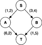
For totally ordered Kleene algebras, the Warshall-Floyd-Kleene algorithm of Section 9.3.1 can be extended to build a so-called predecessor matrix simultaneously to the computation of the matrix closure (Aho et al., 1974). For a pair of variables (S, T) the predecessor matrix P determines the variable X = P(S, T) that is the immediate predecessor of variable T on the optimum path from S to T. The corresponding extension of Algorithm 9.1 is shown in Algorithm 9.2:
Algorithm 9.2 The Warshall-Floyd-Kleene Algorithm with Predecessor Matrix
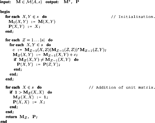
This algorithm still performs the same computations for the closure matrix. Because addition corresponds to maximization with respect to the canonical semiring order, the value MZ(X, Y) in the middle block is set to the larger value between MZ-1(X, Y) and c. In the second case, it means that a better path exists from variable X to variable Y through the intermediate variable Z. We therefore update the predecessor of variable Y according to this new path. Finally, the addition of the matrix MZ with the unit matrix Is in the last block affects the values MZ(X, X) only if 1 > MZ(X, X). It is easy to see that both variations of the Warshall-Floyd-Kleene algorithm adopt equal time and space complexity. The optimum path can then be constructed from the predecessor matrix by recursively enumerating all predecessors. This is illustrated in Example 9.8.
Example 9.8 We take the adjacency matrix of Example 6.2 defined over the tropical semiring of non-negative integers. Here, we identify the graph nodes with letters instead of numbers to prevent confusions with the semiring values. We obtain
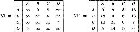
The predecessor matrix obtained from Algorithm 9.2 is
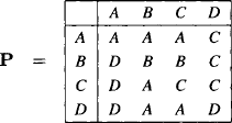
Let us now look for the shortest path from C to B which, according to the closure matrix, has shortest distance 21. We obtain from the predecessor matrix P(C, B) = A. This means that the last visited node just before reaching B on the path from C to B is A. We proceed recursively and obtain P(C, A) = D for the predecessor of A. Finally, P(C, D) = C means that the direct path between C and D also has the shortest distance. Putting things together, the shortest path with distance 21 is
![]()
Given a single matrix with values from a totally ordered Kleene algebra, the extended version of the Warshall-Floyd-Kleene algorithm computes the closure and its associated predecessor matrix with the same computational effort. Based on the predecessor matrix, it is then possible to recursively enumerate each path (X, Y) in linear time to the total number of variables. However, the advantage of using Kleene valuations and local computation for the solution of path problems is the abdication of the explicitly computation of the total matrix and its closure. When we are interested in paths, we must apply a similar strategy to deduce total paths only from the predecessor matrices of smaller subgraphs. For that purpose, we subsequently assume that Kleene valuations consist of pairs of closure and predecessor matrices and start from a knowledgebase {![]() 1, …,
1, …, ![]() n} with
n} with ![]() i = (Mi*, Pi) where Pi corresponds to the predecessor matrix of Mi* obtained from Algorithm 9.2. We define the domain of
i = (Mi*, Pi) where Pi corresponds to the predecessor matrix of Mi* obtained from Algorithm 9.2. We define the domain of ![]() i by d(
i by d(![]() i) = d(Mi*). The projection rule still corresponds to matrix restriction and is applied to both components separately. Here, it is important to note that the values of the projected predecessor matrix may refer to variables that have been eliminated from the domain of the valuation. The combination is executed in the usual way for the closure component. It consists of a component-wise addition of the two extended matrices, followed by the execution of a closure operation. Since we are dealing with a totally ordered Kleene algebra, the component-wise addition of two matrices corresponds to the component-wise maximum, which allows us to initialize the predecessor matrix of the combination. For
i) = d(Mi*). The projection rule still corresponds to matrix restriction and is applied to both components separately. Here, it is important to note that the values of the projected predecessor matrix may refer to variables that have been eliminated from the domain of the valuation. The combination is executed in the usual way for the closure component. It consists of a component-wise addition of the two extended matrices, followed by the execution of a closure operation. Since we are dealing with a totally ordered Kleene algebra, the component-wise addition of two matrices corresponds to the component-wise maximum, which allows us to initialize the predecessor matrix of the combination. For ![]() = (M1*, P1) and ψ = (M2*, P2) with d(
= (M1*, P1) and ψ = (M2*, P2) with d(![]() ) = s, d(ψ) = t and X, Y
) = s, d(ψ) = t and X, Y ![]() d(
d(![]() ) ∪ d(ψ), we compute
) ∪ d(ψ), we compute
![]()
and
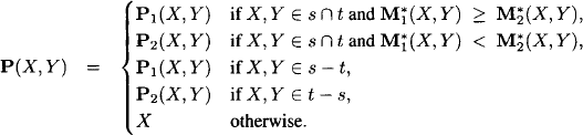
The combined valuation ![]() ⊗ ψ is then obtained by computing the closure of M with P replacing the initialization of the predecessor matrix in Algorithm 9.2. We now observe that this produces a correct predecessor matrix: if computing the closure shows no effect, i.e. if M*(X, Y) = M(X, Y), then P(X, Y) either corresponds to P1(X, Y), P2(X, Y) or X. In the first two cases, the correctness follows from the assumption that
⊗ ψ is then obtained by computing the closure of M with P replacing the initialization of the predecessor matrix in Algorithm 9.2. We now observe that this produces a correct predecessor matrix: if computing the closure shows no effect, i.e. if M*(X, Y) = M(X, Y), then P(X, Y) either corresponds to P1(X, Y), P2(X, Y) or X. In the first two cases, the correctness follows from the assumption that ![]() and ψ are pairs of closures and their corresponding predecessor matrices. The third case is equal to the initialization in Algorithm 9.2. If on the other hand M*(X, Y) ≠ M(X, Y), then some better path was found that goes through some variable Z
and ψ are pairs of closures and their corresponding predecessor matrices. The third case is equal to the initialization in Algorithm 9.2. If on the other hand M*(X, Y) ≠ M(X, Y), then some better path was found that goes through some variable Z ![]() s ∪ t. The algorithm then sets P(X, Y) = P(Z, Y) and the correctness follows by induction.
s ∪ t. The algorithm then sets P(X, Y) = P(Z, Y) and the correctness follows by induction.
Let us now summarize the complete process of computing an optimum path from S to T by local computation. We start from a factorization of Kleene valuations extended by their predecessor matrices, build a covering join tree for this knowledgebase and execute a complete run of the idempotent architecture. We then answer the single-source problem for the variable S by the compilation approach presented above. If ![]() denotes the objective function, we answer the query
denotes the objective function, we answer the query
![]()
from which we obtain the optimum path weight M*(S, T) and the predecessor Z = P(S, T) of T. We proceed recursively by computing the query ![]() ↓{S,Z} and finally obtain the complete path by at most |V| repetitions of this process. It is important to note that once the compilation for the single-source problem is available, no more computations in the valuation algebra are necessary. We thus obtain the path from S to T with a complexity equal to just computing the path weight.
↓{S,Z} and finally obtain the complete path by at most |V| repetitions of this process. It is important to note that once the compilation for the single-source problem is available, no more computations in the valuation algebra are necessary. We thus obtain the path from S to T with a complexity equal to just computing the path weight.
9.4 CONCLUSION
The first part of this chapter deals with sparse, linear systems AX = b with values from a field. Exploiting the sparsity of the matrix A means to limit the number of zero values that change to a non-zero value during the computations. These values are called fill-ins. If no additional structure of the matrix A is present, then ordinary Gaussian elimination with pivoting is performed. This corresponds to computing in the valuation algebra of affine spaces, where the equations are considered as finite representations of the latter. The equations are distributed over the nodes of a join tree, such that the non-zero values in the matrix A are covered by the join tree nodes. Since only these values are involved in the computations, fill-ins are controlled by the join tree. Similar considerations for regular systems lead to LDR-decomposition based on local computation. A second valuation algebra, which is isomorphic to Gaussian potentials, was derived for the case of symmetric, positive definite matrices. Here, the valuations are no more ordinary equations, but they are symmetric, positive definite subsystems themselves. It was shown that such factorizations can either be produced from the matrix, or they occur naturally from specific applications as for example for the normal equations in the least squares method. Local computation with symmetric, positive definite systems required replacing the ordinary distribute phase by a solution construction process. The second part of this chapter focused on fixpoint equation systems X = AX + b with values from a quasi-regular semiring. Such equations frequently occur in path problems and their local computation based solution uses quasi-regular valuation algebras, whose structure is very similar to symmetric, positive definite systems. Consequently, we have a similar solution construction process that follows the usual collect phase of local computation. The second approach was based on Kleene valuation algebras and can be applied to fixpoint systems with values from a Kleene algebra. The application of the idempotent architecture to such knowledgebases lead to a compilation of the path problem into a join tree that qualifies for online query answering.
PROBLEM SETS AND EXERCISES
I.1** We observed in the introduction of Section 9.3.2 that the valuation algebra of linear systems with symmetric, positive definite matrices and the quasi-regular valuation algebra have a very similar structure. Given a symmetric, positive definite system that represents the objective function ![]() , it was shown in Section 9.2.4 how a possible decomposition
, it was shown in Section 9.2.4 how a possible decomposition ![]() =
= ![]() 1 ⊗ … ⊗
1 ⊗ … ⊗ ![]() m can be found. Repeat these considerations for quasi-regular valuation algebras, where the matrices are not necessarily symmetric anymore.
m can be found. Repeat these considerations for quasi-regular valuation algebras, where the matrices are not necessarily symmetric anymore.
I.2** Section 9.3.2 discusses local computation with quasi-regular valuation algebras. This process is very similar to local computation with symmetric, positive definite systems in Section 9.2.2, from which we derived LDLT-decomposition in Section 9.2.3. Show that LDR-decomposition based on local computation is also possible for semiring fixpoint equation systems and thus for quasi-regular valuations. Indication: It is shown in (Backhouse & Carré, 1975) that LDR-decomposition is possible for quasi-regular semirings with idempotent addition. This approach is generalized to quasi-regular semirings in (Radhakrishnan et al., 1992).
I.3 ** In graph related path problems we are often not only interested in the solution of the path problem (e.g. the shortest distance) but also in finding a path that adopts this optimum value (e.g. the shortest paths). At the end of Section 9.3.3 this problem was addressed for Kleene valuation algebras. Provide a similar method that computes paths for quasi-regular valuation algebras.
I.4 ** In the least squares method of Section 9.2.5 the residues are often weighed.
a) Derive the normal equations, if residue Di has weight σi such that
![]()
is to be minimized.
b) More generally, derive the normal equations if DT∑D is to be minimized. The weight matrix ∑ is a positive definite, symmetric matrix.
c) Consider a join tree decomposition of the equations. What conditions must ∑ satisfy in order that the normal equations can be solved by local computation on the join tree?
I.5 ** Reconsider the linear dynamic system from Instance 9.2:
a) Add the equation H3X3 = y3 to the equations in Instance 9.2. How does the estimate of X3 change? This gives the filter solution for X3.
b) Treat this system in the general case for time i = 1, …. n and derive the one-step prediction and the filter solution for Xi.
c) Assume in the dynamic equations and the measurement equations that the residues Di and Ei are weighed with weight matrices Qi and Ri (all positive definite and symmetric). Derive the filter and smoothing solutions in this case.
d) Note that the solution derived so far works if all Ai are regular. No assumption about the rank of Hi is needed. Can you extend the valuation algebra of Section 9.2.1 for non-negative definite, symmetric matrices? Indication: Take (A, Ab) as valuations instead of (A, b). Similar algebras will be studied in Chapter 10.
I.6 ** The equations of the linear dynamic system in Instance 9.2 may also be differently assigned to a join tree: add a node X0 to the left of the join tree in Figure 9.8 and put the equation H0X0 on this node. On the next node X0, X1 put the equations A0X0 − X1 = 0 and H1X1y1 and so forth.
a) Derive the filter solution with this set-up.
b) Derive the smoothing solutions with this set-up.
I.7 *** The exact algebraic relationship between the quasi-regular valuation algebra of Section 6.4 and the symmetric, positive definite valuation algebra of Section 9.2 is yet unknown. The valuations both have a very similar structure, share the same combination rule and also have a related projection rule. On the other hand, there are also important differences, e.g. the quasi-regular valuation algebra provides neutral elements which is not the case in the other algebra. Try to find a common theory for the two algebras.