CHAPTER 3

COMPUTING SINGLE QUERIES

The foregoing chapter introduced the major computational task when dealing with valuation algebras, the inference or projection problem. Also, we gained a first insight into the different semantics that inference problems can adopt under specific valuation algebra instances. The logical next step consists now in the development of algorithms to solve general inference problems. In order to be generic, these algorithms must only be based on the valuation algebra operations without any further assumptions about the concrete, underlying formalism. But before this step, we should also raise the question of whether such algorithms are necessary at all, or, in other words, why a straightforward computation of inference problems is inadequate in most cases. To this end, remember that inference problems are defined by a knowledgebase whose factors combine to the objective function which has to be projected on the actual queries of interest. Naturally, this description can directly be understood as a trivial procedure for the computation of inference problems. However, the reader may have guessed that the complexity of this simple procedure puts us a spoke in our wheel. If the knowledgebase consists of valuations, then, as a consequence of the labeling axiom, computing the objective function results in a valuation of domain . In many valuation algebra instances the size of valuations grows at least exponentially with the size of their domain. And even if the domains grow only polynomially, this growth may be prohibitive. Let us be more concrete and analyse the amount of memory that is used to store a valuation. In Definition 3.3 this measure will be called weight function. Since indicator functions, arithmetic potentials and all their connatural formalisms (see Chapter 5) can be represented in tabular form, their weight is bounded by the number of table entries which corresponds to the number of configurations of the domain. Clearly, this is exponential in the number of variables. Even worse is the situation for set potentials and all instances of Section 5.7 whose weights behave super-exponentially in the worst case. If we further assume that the time complexity of the valuation algebra operations is related to the weight of their factors, we may come to the following conclusion: it is in most cases intractable to compute the objective function explicitly. Second, the domain acts as the crucial point for complexity when dealing with valuation algebras. Consequently, the solution of inference problems is intractable unless algorithms are used which confine the domain size of all intermediate results. This essentially is the promise of local computation that organizes the computations in such a way that domains do not grow significantly. Before we start the discussion of local computation methods, we would like to point out that not all valuation algebras are subject to the above complexity concerns. There are indeed instances that have a pure polynomial behaviour, and this also seems to be the reason why these formalisms have rarely been considered in the context of local computation. However, we will introduce a family of such formalisms in Chapter 6 and also show that there are good reasons to apply local computation to polynomial formalisms.

This first chapter about local computation techniques focuses on the solution of single-query inference problems. We start with the simplest and most basic local computation scheme called fusion or bucket elimination algorithm. Then, a graphical representation of the fusion process is introduced that brings the fundamental ingredient of local computation to light: the important concept of a join tree. On the one hand, join trees allow giving more detailed information about the complexity gain of local computation compared to the trivial approach discussed above. On the other hand, they represent the required structure for the introduction of a second and more general local computation scheme for the computation of single queries called collect algorithms. Finally, we are going to reconsider the inference problem of the discrete Fourier transform from Section 2.3 and show in a case study that applying these schemes reveals the complexity of the fast Fourier transform. This shows that applying local computation may also be worthwhile for polynomial problems.

The fusion or bucket elimination algorithm is a simple local computation scheme that is based on variable elimination instead of projection. Therefore, we first investigate how the operation of projection in a valuation algebra can (almost) equivalently be replaced by the operation of variable elimination.

3.1 VALUATION ALGEBRAS WITH VARIABLE ELIMINATION

The axiomatic system of a valuation algebra given in Chapter 1 is based on a universe of variables r whose finite subsets form the set of domains D. This allows us to replace the operation of projection in the definition of a valuation algebra by another primitive operation called variable elimination which is sometimes more convenient as for the introduction of the fusion algorithm. Thus, let be a valuation algebra with D = P(r) and Φ being the set of all possible valuations with domains in D. For a valuation Φ and a variable X d(), we define

(3.1)

Some important properties of variable elimination, that follow from this definition and the valuation algebra axioms, are pooled in the following lemma:

Lemma 3.1

Proof:

According to equation (3.3) variables can be eliminated in any order with the same result. We may therefore define the consecutive elimination of a non-empty set of variables s = {X1, …, Xn} d() unambiguously by

(3.5)

This, on the other hand, permits expressing any projection by the elimination of all unrequested variables. For x d{}, we have

(3.6)

To sum it up, equation (3.1) and (3.6) allow switching between projection and variable elimination ad libitum. Moreover, we may, as an alternative to definitions in Chapter 1, define the valuation algebra framework based on variable elimination instead of projection (Kohlas, 2003). Then, the properties in the above lemma replace their counterparts based on projection in the new axiomatic system, and projection can later be derived using equation (3.6) and the additional domain axiom (Shafer, 1991).

3.2 FUSION AND BUCKET ELIMINATION

The fusion (Shenoy, 1992b) and bucket elimination (Dechter, 1999) algorithms are the two simplest local computation schemes for the solution of single-query inference problems. They are both based on successive variable elimination and correspond essentially to traditional dynamic programming (Bertele & Brioschi, 1972). Applied to the valuation algebra of crisp constraints, bucket elimination is also known as adaptive consistency (Dechter & Pearl, 1987). We will see in this section that fusion and bucket elimination perform exactly the same computations and are therefore equivalent. On the other hand, their description is based on two different but strongly connected graphical structures that bring the two important perspectives of local computation to the front: the structural buildup of inference problems that makes local computation possible and the concept that determines its complexity. This section introduces both algorithms separately and proves their equivalence such that later considerations about complexity apply to both schemes at once. In doing so, we provide a slightly more general introduction which is not limited to queries consisting of single variables, as it is often the case for variable elimination schemes.

3.2.1 The Fusion Algorithm

Let be a valuation algebra with the operation of projection replaced by variable elimination. We further assume an inference problem given by its knowledgebase and a single query where denotes the joint valuation . The domain d() must correspond to a set of variables {X1, …, Xn} with n = |d()|. The fusion algorithm (Shenoy, 1992b; Kohlas, 2003) is based on the important property that eliminating a variable X d() only affects the knowledgebase factors whose domains contain X. This is the statement of the following theorem:

Theorem 3.1 Consider a valuation algebra and a factorization with i and 1 ≥ i ≤ m. For X d() we have

(3.7)

Proof: This theorem is a simple consequence of Lemma 3.1, Property 3. Since combination is associative and commutative, we may always write

We therefore conclude that eliminating variable X only requires combining the factors whose domains contain X. According to the labeling axiom, this creates a new factor of domain

(3.8)

that generally is much smaller than the total domain d() of the objective function. The same considerations now apply successively to all variables that do not belong to the query x d(). This procedure is called fusion algorithm (Shenoy, 1992b) and can formally be defined as follows: let Fusy({1, …, m}) denote the set of valuations after fusing {1, …, m} with respect to variable Y d(1) … d(m),

(3.9)

where

Using this notation, the result of Theorem 3.1 can equivalently be expressed as:

(3.10)

By repeated application and the commutativity of variable elimination we finally obtain the fusion algorithm for the computation of a query x; d(). If {Y1, …, Yk} = d() - x are the variables to be eliminated, we have

(3.11)

This is a generic algorithm for solving the single-query inference problem over an arbitrary valuation algebra as introduced in Chapter 1. Algorithm 3.1 provides a summary of the complete fusion process which stands out by its simplicity and compactness. Also, Example 3.1 expands the complete computation of fusion for the inference problem of Instance 2.1.

Algorithm 3.1 The Fusion Algorithm

Example 3.1 To exemplify the fusion algorithm, we reconsider the inference problem of the Bayesian network from Instance 2.1. The knowledgebase consists of eight valuations with domains: d(1) = {A}, d(2) = {A, T}, d(3) = {L, S}, d(4) = {B, S}, d(5) = {E,L,T}, d(6) = {E, X}, d(7) = {B,D,E} and d(8) = {S}. We choose {A, B, D} as query and eliminate all variables from {E, L, S, T, X} in the elimination sequence (X, S, L, T, E):

Elimination of variable X:

Elimination of Variable S:

Elimination of Variable L:

Elimination of Variable T:

Elimination of Variable E:

We next present a graphical representation of the fusion process proposed by (Shafer, 1996). For this purpose, we maintain a set of domains that is initialized with the domains of all knowledgebase factors l = {d(1), …, d(m)}. In parallel, we build up a labeled graph (V, E, λ, D) which is assumed to be empty at the beginning, i.e. V = and E = . When variable Xi is eliminated during the fusion process, we remove all domains from the set l that contain variable Xi and compute their union

(3.12)

We then add the new domain si - {Xi} to the set l which altogether updates to

This corresponds to the i-th step of the fusion algorithm where variable Xi d() - x is eliminated. Then, a new node i is constructed with label λ(i) = sj. This node is tagged with a color and added to the graph. We then go through all other colored graph nodes: if the label of such a node v V contains the variable Xi, then its color is removed and a new edge {i, v} is added to the graph. This whole process is repeated for all variables d() - x to be eliminated. Finally, one last finalization step has to be performed, which corresponds to the combination in equation (3.11): at the end of the variable elimination process, the set l will not be empty. It consists either of the query variables that are never eliminated, or, if the query is empty, it contains an empty set. We therefore add a last, colored node to the graph whose domain corresponds to the union of all remaining elements in the domain set. Then, we link all nodes that are still tagged with a color to this new node and remove all node colors. Algorithm 3.2 gives a summery of the whole construction process and returns a labeled graph (V, E, λ, D). Since all node labels created during the graph construction process consist of the variables from d(), we may always set D = P(d(λ)). The yet mysterious name of this algorithm will be explained subsequently.

Algorithm 3.2 Join Tree Construction

Example 3.2 We give an example of the graphical representation of the fusion algorithm based on the factor domains of the Bayesian network example from Instance 2.1. At the beginning, we have l = {{A}, {A, T}, {L, S}, {B, S}, {E, L, T}, {E, X}, {B, D, E}, {S}}. The query of this inference problem is {A, B, D} and the variables {E, L, S, T, X} have to be eliminated. We choose the elimination sequence (X, S, L, T, E) as in Example 3.1 and proceed according to the above description. Colored nodes are represented by a dashed border.

• Elimination of variable X:
  
• Elimination of variable S:
  
• Elimination of variable L:
  
• Elimination of variable T:
  
• Elimination of variable E:
  
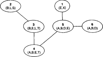
• End of variable elimination: after the elimination of variable E, only the last added node {A, B, E, D} is colored. This, however, is due to the particular structure of our knowledgebase, and it is quite possible that multiple colored nodes still exist after the elimination of the last variable. We next enter the finalization step and add a last node whose label corresponds to the union of the remaining elements in the domain list, i.e. {A} and {A, B, D}. This node is then connected to the colored node and all colors are removed. The result of the construction process is shown in Figure 3.1.

3.2.2 Join Trees

Let us investigate the graphical structure that results from the fusion process in more detail. We first remark that each node can be given the number of the eliminated variable. For example, in Figure 3.1 the node labeled with {B, E, L, T} has number 3 because it was introduced during the elimination of the third variable that corresponds to L in the elimination sequence. This holds for all nodes except the one added in the finalization step. We therefore say that variable Xi has been eliminated in node i for 1 ≤ i ≤ |d() - x|. If we further assign number |d() - x| + 1 to the finalization node, we see that if i < j implies that node j has been introduced after node i.

Lemma 3.2 At the end of the fusion algorithm the graph G is a tree.

Proof: During the graph construction process, only colored nodes are connected, which always causes one of them to lose its color. It is therefore impossible to create cycles. But it may well be that different (unconnected) colored nodes exist after the variable elimination process. Each of them is part of an independent tree, and each tree contains exactly one colored node. In the finalization step, we add a further node and connect it with all the remaining colored nodes. The total graph G must therefore be a tree to which all nodes are connected.

This tree further satisfies the running intersection property which is sometimes also called Markov property or simply join tree property. Accordingly, such trees are named join trees, junction trees or Markov trees.

Definition 3.1 A labeled tree (V, E, λ, D) satisfies the running intersection property if for two nodes i, j V and X λ(i) λ(j), X λ(k) for all nodes k on the path between i and j.

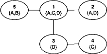
Example 3.3 Figure 3.2 reconsiders the tree G2 from Example 2.1 equipped with a labeling function λ for r = {A, B, C, D}. The labels are: λ(1) = {A, C, D}, λ(2) = {A, D}, λ(3) = {D}, λ(4) = {C} and λ(5) = {A, B}. This labeled tree is not a join tree since C λ(1) λ(4) but C λ(3). However, adding variable C to node label λ(3) will result in a join tree.

Lemma 3.3 At the end of the fusion algorithm the graph G is a join tree.

Proof: We already know that G is a tree. Select two nodes s′ and s″ and . We distinguish two cases: If X does not belong to the query, then X is eliminated in some node. We go down from s′ along to later nodes, until we arrive at the node where X is eliminated. Let k′ be the number of this node. Similarly, we go down from s″ to later nodes until we arrive at the elimination node of X. Assume the number of this node to be k". But X is eliminated in exactly one node. So k′ = k″ and the path from s′ to s″ goes from s′ to k′ = k″ and from there to s". X belongs to all nodes of the paths from s′ to k′ = k″ and s″ to k′ = k", hence to all nodes of the path from s′ to s". The second possibility is that X belongs to the query. Then, X has never been eliminated but belongs to the label of the node added in the finalization step. Thus, the two paths meet in this node and the same argument applies.

Example 3.4 In Figure 3.1, variable E is eliminated in node 5 but appears already in node 3, therefore it must also belong to the label of node 4. On the other hand, variable B belongs to the query and is therefore part of the node label introduced in the finalization step. This is node number 6. But variable B also appears in node 2 and therefore does so in the nodes 3 to 5.

3.2.3 The Bucket Elimination Algorithm

We reconsider the same setting for the introduction of bucket elimination: let be a valuation algebra with the operation of projection replaced by variable elimination. The knowledgebase of the inference problem is {1, …, m} Φ and x d() = {X1, …, Xn} denotes the single query. Similarly to the fusion algorithm, the bucket elimination scheme (Dechter, 1999) is based on the important observation of Theorem 3.1 that eliminating a variable only affects the valuations whose domain contain this variable. We again choose an elimination sequence (Y1, …, Yk) for the variables in d() - x and imagine a bucket for each of these variables. These buckets are ordered with respect to the variable elimination sequence. We then partition the valuations in the knowledgebase as follows: all valuations whose domain contains the first variable Y1 are placed in the first bucket, which we subsequently denote by bucket1. This process is repeated for all other buckets, such that each valuation is placed in the first bucket that mentions one of its domain variables. It is not possible that a valuation is placed in more than one bucket, but there may be valuations whose domain is a subset of the query and therefore do not fit in any bucket. Bucket elimination then proceeds as follows: at step i = 1, …, k - 1, bucketi is processed by combining all valuations in this bucket, eliminating variable Yi from the result and placing the obtained valuation in the first of the remaining buckets that mentions one of its domain variables. At then end, we combine all valuations contained in bucketk with the remaining valuations of the knowledgebase for which no bucket was found in the initialization process.

In the first step of the bucket elimination process, bucket1 computes

and moves the result into the next bucket that contains one of its domain variables. This corresponds exactly to equation (3.9) whereas

In other words, the first step of the bucket elimination process corresponds to the first step of the fusion algorithm, and the same holds also naturally for the remaining steps. Bucket elimination therefore computes equation (3.11) that implies its correctness and the equivalence to the fusion algorithm.

Theorem 3.2 Fusion and bucket elimination with identical elimination sequences perform exactly the same computations.

Example 3.5 We repeat the computations of Example 3.1 and 3.2 from the perspective of bucket elimination. The knowledgebase consists of eight valuations with domains: d(1) = {A}, d(2) = {A, T}, d(3) = {L, S}, d(4) = {B, S}, d(5) = {E, L, T}, d(6) = {E, X}, d(7) = {B, D, E} and d(8) = {S}. The query is {A, B, D}. We choose the same elimination sequence (X, S, L, T, E), construct a bucket for each variable in the elimination sequence and partition the valuations accordingly. Since d(1) x, 1 is not contained in any bucket.

Initialization:

Elimination of bucket X:

Elimination of bucket S:

Elimination of bucket L:

Elimination of bucket N:

Elimination of bucket E:

Combining this with valuation 1 confirms the result of Example 3.2.

Similar to the fusion algorithm, we give a graphical representation of the bucket elimination process. We first create a graph node for each bucket and label it with the corresponding variable. If during the elimination of bucketX a valuation is added to bucketY, then an edge {X, Y} is added to the graph. Since the elimination of each bucket generates exactly one new valuation that is added to the bucket of a variable which follows later in the elimination sequence, the resulting graph will always be a tree called bucket-tree. The bucket-tree of Example 3.5 is shown in Figure 3.3.

Based on the bucket-tree, we can derive the join tree that underlies the bucket elimination process. We revisit each bucket at the time of its elimination and compute the union domain of all valuations contained in this bucket. This domain is assigned as label to the corresponding node in the bucket tree. Finally, we add a new node with the query of the inference problem as label to the modified bucket-tree and connect this node with the node that belongs to the last variable in the elimination sequence. It follows from Theorem 3.2 and Lemma 3.3 that the resulting graph is a join tree, i.e. we obtain the same join tree as for the fusion algorithm.

Example 3.6 At the time of elimination, the buckets of Example 3.5 contain valuations over the following variables:

We next assign these domains as labels to the corresponding nodes in the bucket-tree. Finally, we create a new node with the query domain {A, B, D} and connect it to the node that refers to the last variable in the elimination sequence. The resulting graph is shown in Figure 3.4. If we further replace the variables from the bucket-tree by their position in the elimination sequence and assign number k + 1 to the node with the query domain, we obtain the join tree of Figure 3.1.

Our presentation of the bucket elimination algorithm differs in two points from the usual way that it is introduced. First, we consider arbitrary query sets with possibly more than one variable. Consequently, there may be valuations that cannot be assigned to any bucket as shown in Example 3.5, and this makes it necessary to add the additional query node when deriving the join tree from the bucket-tree. The second difference concerns the elimination sequence. In the literature, buckets are normally processed in the inverse order to the elimination sequence. This however is only a question of terminology. Before we turn towards a complexity analysis of the fusion or bucket elimination algorithm, we reconsider the computational task of Example 1.2 used to illustrate the potential benefit of local computation in the introduction of this book.

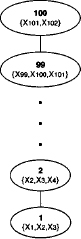
Example 3.7 The formalism used in Example 1.2 in the introduction consists of mappings from configurations to real numbers. Combination refers to point-wise multiplication and projection to summing up the values of the eliminated variables. In other words, this formalism corresponds to the valuation algebra of arithmetic potentials. The knowledgebase is given by the set of function {f1, …, f100} and the query is {X101, X102}. We recall that an explicit computation of the objective function is impossible. Instead, we apply the fusion or bucket elimination algorithm to this inference problem with the elimination sequence (X1, …, X100). This leads to the join tree shown in Figure 3.5, and the executed computations correspond to equation (I.3). Thus, the domains of all intermediate factors that occur during the computations contain at most three variables.

3.2.4 First Complexity Considerations

Making a statement about the complexity of local computation for arbitrary valuation algebras is impossible since we do not have information about the form of valuations. Remember, the valuation algebra framework describes valuations only by their operational behaviour. We therefore restrict ourselves first to a particular class of valuations and show later how the corresponding complexity considerations can be generalized. More concretely, we focus on valuations that are representable in tabular form such as indicator functions from Instance 1.1 or arithmetic potentials from Instance 1.3. In fact, we shall study in Chapter 5 the family of semiring valuation algebras which all share this common structure of mapping configurations to specific values. Thus, given the universe of variables with finite frames, we denote by the size of the largest variable frame. Then, the space (subsequently called weight) of a valuation with domain d() = s is bounded by and similar statements can be made about the time complexity of combination and projection.

When during the fusion process variable Xi d()-x is eliminated, all valuations are combined whose domain contains this variable according to equation (3.9). Then, variable Xi is eliminated. Thus, if mi valuations contain variable Xi before iteration i of the fusion algorithm, its elimination requires mi, - 1 combinations and one variable elimination (projection). The domain si of the valuation resulting from the combination sequence is given in equation (3.12). We may therefore say that during the elimination of variable Xi, the time complexity of each operation is bounded by which gives us the following total time complexity for the fusion or bucket elimination process:

In the graphical representation of the fusion algorithm, the elimination of variable Xi introduces a new join tree node with label λ(i) = si. The size of these labels are bounded by the largest node label . A related measure called treewidth will be introduced in Definition 3.2 below. Further, we observe that the fusion process reinserts a valuation into its current knowledgebase after the elimination of each variable. This valuation was called ψ in equation (3.9). We may therefore say that Σ mi ≤ m + |d() - x| ≤ m + |d()| where m denotes the size of the original knowledgebase of the inference problem and x the query. Putting things together, we obtain the following simplified expression for the time complexity:

(3.13)

Slightly better is the space complexity. During the elimination of variable Xi a sequence of combinations is computed that creates an intermediate result with domain si, from which the variable Xi is eliminated. In case of valuations with a tabular representation, the intermediate result does not need to be computed explicitly. This will be explained in more detail in Section 5.6. Here, we content ourselves with the rather intuitive idea that each value (or table entry) of this intermediate valuation can be computed separately and directly projected. This omits the computation of the complete intermediate valuation and directly gives the result after eliminating variable Xi from the combination. The domain size of this valuation is si - {Xi} ≤ ω - 1, and its size is therefore bounded by . Further, we have just seen that the number of eliminations is at most |d()| which gives us a total space complexity of

(3.14)

It is important to remark that both complexities depend on the shape of the join tree, respectively on its largest node label called treewidth. This measure varies under different elimination sequences as illustrated in the following example.

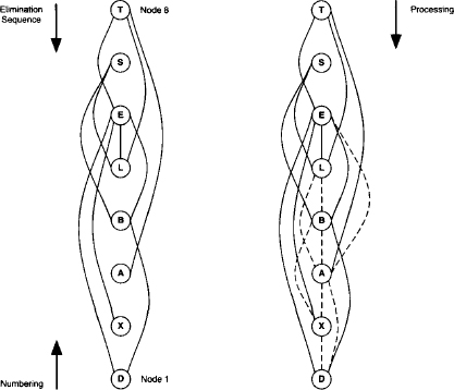
Example 3.8 Figure 3.6 shows two different join trees for the domain list of Example 3.2 obtained by varying the elimination sequence. In order to get comparable results, we take the empty set as query and eliminate all variables using Algorithm 3.2. The left-hand join tree is obtained from the elimination sequence (T, S, E, L, B, A, X, D) and has ω = 6. The right-hand join tree has ω = 3 due to the clever choice of the elimination sequence (A, T, S, L, B, E, X, D). After a certain number of variable elimination steps only a single valuation remains in both examples from which one variable after the other is eliminated. This uninteresting part is omitted in the join trees of Figure 3.6. A third join tree with ω = 4 can be obtained by eliminating the remaining variables in Example 3.2. This corresponds to the elimination sequences that start with (X, S, L, T, E)

The complexity of solving an inference problem with the fusion algorithm therefore depends on the variable elimination sequence that produces a join tree whose largest node label should be as small as possible. This follows from equation (3.13) and (3.14). In order to understand how elimination sequences and the treewidth measure are related, we consider the primal graph of the inference problem introduced in Section 2.1. Since a primal graph contains a node for every variable, an elimination sequence can be represented by a particular node numbering. Here, we number the nodes with respect to the inverse elimination sequence as shown on the left-hand side of Figure 3.7. Such graphs are called ordered graphs, and we define the width of a node in an ordered graph as the number of its earlier neighbors. Likewise, we define the width of an ordered graph as the maximum node width. Next, we construct the induced graph of the ordered primal graph by the following procedure: process in the reversed order of the node numbering (i.e. according to the elimination sequence) and add edges to ensure for each node that its earlier neighbors are directly connected. We define the induced width of an elimination sequence (or ordered graph) as the width of its induced graph and refer to the induced width of a graph ω* as the minimum width over all possible elimination sequences (orderings) (Dechter & Pearl, 1987). Since a primal graph is associated with each inference problem, we may also speak about the induced width of an inference problem.

Example 3.9 The left-hand part of Figure 3.7 shows the primal graph of Example 3.2 ordered with respect to the elimination sequence (T, S, E, L, B, A, X, D). Node E has width 4 since four neighbors posses a smaller node number. Then, the right-hand part of Figure 3.7 shows its induced graph. Here, node E has 5 neighbors {A, B, D, L, X} with a smaller number which also determines the width of this elimination sequence. Observe that this corresponds to the largest node label of the join tree on the left-hand side of Figure 3.6, if we add the variable E that has been eliminated in this node.

The following theorem has been proved by (Arnborg, 1985):

Theorem 3.3 The largest node label in a join tree equals the induced width of the elimination sequence plus one.

This relationship allows us subsequently to focus only on join trees when dealing with complexity issues. It is then common to use a second but equivalent terminology called treewidth, which has been introduced by (Robertson & Seymour, 1983; Robertson & Seymour, 1986):

Definition 3.2 The treewidth of a join tree (V, E, λ, D) is given by

(3.15)

and we refer to the minimum treewidth over all join trees created from all possible variable elimination sequences as the treewidth of the inference problem.

Since treewidth and induced width are equal according to the above theorem, we reuse the notation ω* for the treewidth of an inference problem. It is very important to distinguish properly between the two notions treewidth of a join tree and treewidth of an inference problem. The first refers to a concrete join tree whereas the second captures the best join tree over all possible elimination sequences of a given inference problem. The decrement in equation (3.15) ensures that inference problems whose primal graphs are trees have treewidth one. Besides induced width and treewidth, there are other equivalent characterization in the literature. Perhaps most common among them is the notion of a partial k-tree (van Leeuwen, 1990).

Example 3.10 The value ω from Example 3.8 refers to the incremented treewidth of the join tree. We therefore have in this example three join trees of treewidth 2, 3 and 5 and conclude that the treewidth of the medical inference problem with empty query is at most 2. In fact, it is equal to 2 because one of the knowledgebase factors has a domain of three variables, which makes it impossible to get a lower treewidth.

Returning to the task of identifying the complexity of the fusion and bucket elimination algorithm, we obtain a complexity bound for the solution of a single-query inference problem by including the treewidth ω* of the latter into equation (3.13) and (3.14):

(3.16)

This is called a parameterized complexity (Downey & Fellows, 1999) with the treewidth of the inference problem as parameter. Naturally, the question arises how the minimum treewidth over all possible variable elimination sequences can be found, the more so as it determines the complexity of applying the fusion and bucket elimination algorithm. Concerning this important question we only have bad news. It has been shown by (Arnborg et al., 1987) that finding the smallest treewidth of a graph is NP-complete. In fact, the task of deciding if the primal graph of the inference problem has a treewidth below a certain constant k can be performed in O(|d()| · g(k)) where g(k) is a very bad exponential function in k (Bodlaender, 1998; Bodlaender, 1993). Fortunately, there are good heuristics for this task that deliver join trees with reasonable treewidths as we will see in Section 3.7. It is thus important to distinguish the two ways of specifying the complexity of local computation schemes. Given a concrete join tree or an elimination sequence with treewidth ω, we insert this value into equation (3.16) and obtain the achieved complexity of a concrete run of the fusion algorithm. On the other hand, using the treewidth ω* of the inference problem in these formulae denotes the best complexity over all possible join trees or variable elimination sequences that could be achieved for the solution of this inference problem by the fusion or bucket elimination algorithm. But since we are generally not able to exactly determine this value, this often remains an unsatisfied wish. However, it is nevertheless common to specify the complexity of local computation schemes by the treewidth of the inference problem and we will also go along with this.

3.2.5 Some Generalizing Complexity Comments

At the beginning of our complexity considerations we limited ourselves to a family of valuation algebras whose elements are representable in tabular form. These formalisms share the property that the size of valuations grows exponentially with the size of their domains. Thus, the space of a valuation with domain s = d() is bounded by O(d|s|) where d denotes the size of the largest variable frame. Similar statements were made about the time complexity of combination and projection. This view is too restrictive, since there are many other valuation algebra instances that do not keep with this estimation. On the other hand, there are also examples where it is unreasonable to measure time and space complexity by the same function as it has been done in equation (3.16). Examples of such formalisms will be given in Chapter 6. However, a general assumption we are allowed to make is that the space of a valuation and the execution time for the operations shrink under projection. Remember, the idea of local computation is to confine the domain size of intermediate factors during the computations. If this assumption could not be made, local computation would hardly be a reasonable approach.

Definition 3.3 Let be a valuation algebra. A function is called weight function if for all Φ and x d() we have .

Weight functions are still too general to be used for complexity considerations. In many cases however, we can give a predictor for the weight function which is only based on the valuation’s domain. Such weight predictable valuation algebras share the property that the weight of a valuation can be estimated from its domain only.

Definition 3.4 A weight function ω of a valuation algebra is called weight predictor if there exists a function such that for all Φ

We give some examples of weight functions and weight predictors for the valuation algebras introduced in Chapter 1:

Example 3.11

• A weight predictor for the valuation algebra of arithmetic potentials that also applies to indicator functions and all formalisms of Section 5.3 has already been used in equation (3.16):

(3.17)

where s = d() denotes the domain of valuation and

the largest variable frame. Observe that in this particular case, we could also use the weight function directly as weight predictor since it depends only on the valuation’s domain.

• A reasonable and often used weight function for relations is ω() = |d()| · card(), where card() stands for the number of tuples in . Regrettably, this is not a weight predictor itself since the number of tuples cannot be deduced from the relation’s domain.
• Finally, a weight predictor for the valuation algebra of set potentials and all formalisms of Section 5.7 is

(3.18)

Observe that we presuppose binary variables in this formula.

Subsequently, we will use weight predictors for the analysis of the time and space complexity of local computation. This allows us to make more general complexity statements that can then be specialized to a specific formalism by choosing an appropriate weight predictor. Further, we use two different weight predictors f and g for time and space complexity. This accounts for the observation that time and space complexity cannot necessarily be estimated by the same function, but both satisfy the fundamental property that they are non-increasing under projection. We obtain for the general time complexity of the fusion and bucket elimination algorithm:

(3.19)

This follows directly from equation (3.16). Remember that the assumption of valuations with a tabular representation allowed us to derive a lower space complexity in equation (3.16). This optimization cannot be performed for arbitrary valuation algebras. For the elimination of variable Xi we therefore need to compute the combinations first, which results in an intermediate factor with domain size |λ(i)| ≤ ω* + 1. Then, the variable Xi can be eliminated and the result is added to the knowledgebase. Altogether, this gives us the following general space complexity of the fusion and bucket elimination algorithm:

(3.20)

Clearly, for the case of applying the fusion algorithm to arithmetic potentials, indicator functions and all other formalism of Section 5.3, we may choose the same weight predictor of equation (3.17) for both time and space complexity. Moreover, the space complexity can then be improved to the one given in equation (3.16). This shows the difficulties of making general complexity statements for local computation applied to unspecified valuation algebras.

3.2.6 Limitations of Fusion and Bucket Elimination

The fusion or bucket elimination algorithm is a generic local computation scheme to solve single-query inference problems in a simple and natural manner. Nevertheless, it has some drawbacks compared to other local computation procedures that will be introduced below. Here, we address two important points of criticism:

• The fusion or bucket elimination algorithm can be applied to each formalism that satisfies the valuation algebra axioms from Section 1.1. But we have also seen in Appendix A.2 of Chapter 1 that there exists a more general definition of the axiomatic framework which is based on general lattices instead of variable systems. Fusion and bucket elimination require variable elimination and can therefore not be generalized to valuation algebras on arbitrary lattices.
• Time and space complexity of the fusion algorithm are bounded by the treewidth of the inference problem, which makes the application difficult when join trees have large labels. Experiments from constraint programming (Larrosa & Morancho, 2003) show that the space requirement is particularly sensitive, for which reason inference is often combined with search methods that only require linear space. However, search methods need more structure than offered by the valuation framework. We refer to (Rossi et al., 2006) for a survey of such trading or hybrid methods in constraint programming. Looking at equation (3.20), we observe that the function arguments of the two terms distinguish in a constant number. We will see later that this is a consequence of the particular join trees that emerge from the fusion and bucket elimination process. Further, we know that the first term vanishes when dealing with particular valuation algebras. It will be shown in Section 5.3 that this also includes constraint systems. To make local computation more space efficient for such formalisms, we therefore aim at reducing the argument of the second term in equation (3.20).

In the subsequent sections, we present an alternative picture of local computation that finally leads to a second algorithm for the solution of single-query inference problems that does not depend on variables anymore and which may also provide a better space performance. The essential difference with respect to the fusion algorithm is that the join tree construction is decoupled from the actual inference process. Instead, a suitable join tree for the current inference problem is initially constructed, and local computation is then described as a message-passing process where nodes act as virtual processors and collaborate by exchanging messages. The key advantage of this approach is that we no longer depend on the very particular join trees that are obtained from the fusion algorithm. To study the requirements for a join tree to serve as local computation base, we first introduce a specialized class of valuation algebras that provide neutral information pieces. It will later be shown in Section 3.10 that the existence of such neutral elements is not mandatory for the description of local computation as message-passing scheme. But if they exist, the discussion simplifies considerably. Moreover, neutral elements are also interesting in other contexts that will be discussed in later parts of this book.

3.3 VALUATION ALGEBRAS WITH NEUTRAL ELEMENTS

Following the view of a valuation algebra as a generic representation of knowledge or information, some instances may exist that contain pieces that express vacuous information. In this case, such a neutral element must exist for every set of questions SD and must therefore be contained in every subsemigroup Φs of Φ. If we then combine those pieces with already existing knowledge of the same domain, we do not gain new information. Hence, there is an element for every subsemigroup Φs such that = es = for all Φs. We further add a neutrality axiom to the valuation algebra system which states that a combination of neutral elements leads to a neutral element with respect to the union domain.

Definition 3.5 A valuation algebra has neutral elements, if for every domain s D there exists an element es Φs such that es = es = for all Φs. These elements must satisfy the following property:

(A7) Neutrality: For x,y D,

(3.21)

If neutral elements exist, they are unique within the corresponding subsemigroup. In fact, suppose the existence of another element with the identical property that for all Φs. Then, since es and behave neutrally among each other, . Furthermore, valuation algebras with neutral elements allow for a simplified version of the combination axiom that was already proposed in (Shenoy & Shafer, 1990).

Lemma 3.4 In a valuation algebra with neutral elements, the combination axiom is equivalently expressed as:

(A5) Combination: For with ,

(3.22)

Proof: Equation (3.22) follows directly from the combination axiom with z = x. On the other hand, let . Since we derive from equation (3.22) and Axiom (A1) that

The last equality holds because

Note that this result presupposes the distributivity of the lattice D.

The following lemma shows that neutral elements also behave neutral with respect to valuations on larger domains:

Lemma 3.5 For Φ with d() = x and y x it holds that

(3.23)

Proof: From the associativity of combination and the neutrality axiom follows

The presence of neutral elements allows furthermore to extend valuations to larger domains. This operation is called vacuous extension and may be seen as a dual operation to projection. For Φ and d() y we define

(3.24)

Before we consider some concrete examples of valuation algebras with and without neutral elements, we introduce another property called stability that is closely related to neutral elements. In fact, stability can either be seen as the algebraic property that enables undoing the operation of vacuous extension, or as a strengthening of the domain axiom (A6).

3.3.1 Stable Valuation Algebras

The neutrality axiom (A7) determines the behaviour of neutral elements under the operation of combination. It states that a combination of neutral elements will always result in a neutral element again. However, a similar property can also be requested for the operation of projection. In a stable valuation algebra, neutral elements always project to neutral elements again (Shafer, 1991). This property seems natural but there are indeed important examples which do not fulfill stability.

Definition 3.6 A valuation algebra with neutral elements is called stable if the following property is satisfied for all x,y D with x y,

(A8) Stability:

(3.25)

Stability is a very strong condition which also implies other valuation algebra properties: together with the combination axiom, it can, for example, be seen as a strengthening of the domain axiom. Also, it is possible to revoke vacuous extension under stability. These are the statements of the following lemma:

Lemma 3.6

(3.26)

Proof:

3.1 Neutral Elements and Indicator Functions

In the valuation algebras of indicator functions, the neutral element for the domain s D is given by es(x) = 1 for all x Ωs. We then have for Φs

Also, the neutrality axiom holds, since for s,t D with we have

Finally, the valuation algebra of indicator functions is also stable. For s,t D with s t and x Ωs it holds that

3.2 Neutral Elements and Arithmetic Potentials

Arithmetic potentials and indicator functions share the same definition of combination. We may therefore conclude that arithmetic potentials also provide neutral elements. However, in contrast to indicator functions, arithmetic potentials are not stable. We have for s,t D with s t and × Ωs

3.3 Neutral Elements and Set Potentials

In the valuation algebra of set potentials, the neutral element es for the domain s D is given by es(A) = 0 for all proper subsets A Ωs and es(Ωs) = 1. Indeed, it holds for Φ with d() = s that

The second equality follows since for all other values of C we have es(C) = 0. Also, the neutrality axiom holds which will be proved explicitly in Section 5.8.1. Further, set potentials are stable. For s,t D and s t it holds that

The second equality holds because et(Ωt) = 1 is the only non-zero summand.

3.4 Neutral Elements and Relations

For s D the neutral element in the valuation algebra of relations is given by es = Ωs. Similar to indicator functions these neutral elements are also stable. However, there is an important issue regarding neutral elements in the relational algebra. Since variable frames are often very large or even infinite (i.e. all possible strings), the neutral elements can sometimes not be expressed explicitly.

3.5 Neutral Elements and Density Functions

Equation (1.15) introduced the combination of density functions as simple multiplication. Therefore, the definition would clearly meet the requirements for a neutral element. However, this function es is not a density since its integral will not be finite

Hence, densities form a valuation algebra without neutral elements. This holds in particular also for Gaussian potentials in Instance 1.6.

Before we continue with the interpretation of the fusion algorithm as a message-passing scheme in Section 3.5, we introduce a second family of elements that may be contained in a valuation algebra. As neutral elements express neutral knowledge, null elements express contradictory knowledge with respect to their domain.

3.4 VALUATION ALGEBRAS WITH NULL ELEMENTS

Some valuation algebras contain elements that express incompatible, inconsistent or contradictory knowledge according to questions s D. Such valuations behave absorbingly for combination and are therefore called absorbing elements or null elements. Hence, in a valuation algebra with null elements there is an element zs Φs such that zs = zs = zs for all Φs. We call a valuation Φs consistent, if and only if ≠ zs. It is furthermore a very natural claim that a projection of some consistent valuation produces again a consistent valuation. This requirement is captured by the following additional axiom.

(A9) Nullity: For x, y D, x y and Φy,

if, and only if, = zy.

In other words, if some valuation projects to a null element, then it must itself be a null element. Thus, contradictions can only be derived from contradictions. We further observe that according to the above definition, null elements absorb only valuations of the same domain. In case of stable valuation algebras, however, this property also holds for any other valuation.

Lemma 3.7 In a stable valuation algebra with null elements we have for all Φ with d() = x and y D

(3.27)

Proof: We remark first that from equation (3.26) it follows

Hence, we conclude from the nullity axiom that and derive

Let us search for null elements in the valuation algebra instances of Chapter 1.

3.6 Null Elements and Indicator Functions

In the valuation algebras of indicator functions the null element for the domain s D is given by zs(x) = 0 for all x Ωs. We then have

Since projection refers to maximization, it is easy to see that null elements, and only null elements project to null elements.

3.7 Null Elements and Arithmetic Potentials

Again, since their combination rules are equal, arithmetic potentials and indicator functions share the same definition of null elements: for s D we define zs(x) = 0 for all x Ωs. The absorption property for combination follows directly from Instance 3.6. Further, projection is defined as summation for arithmetic potentials and since the values are non-negative, it is again only the null element that projects to a null element.

3.8 Null Elements and Relations

Since we have already identified the null elements in the valuation algebra of indicator functions, it is simple to give way to relations. Due to equation (1.9) null elements are simply empty relations with respect to their domain.

3.9 Null Elements and Set Potentials

In the valuation algebra of set potentials, the null element zs for the domain s r is defined by zs(A) = 0 for all A Ωs. These elements behave absorbingly for combination, and are the only elements that project to null elements, which follows again from their non-negative values. Although this is rather easy to see, we will give a formal proof in Section 5.8.2.

3.10 Null Elements and Density Functions

In the valuation algebra of density functions, the null element for the domain s is given by zs(x) = 0 for all x Ωs. The properties of null elements follow again from the fact that density functions are non-negative.

3.11 Null Elements and Gaussian Densities

In the introduction of density functions we also mentioned that the family of Gaussian densities forms a subalgebra of the valuation algebra of density functions. Although we are going to study this formalism extensively in Chapter 10, we already point out that Gaussian densities do not possess null elements due to the requirement for a positive definite concentration matrix.

Null elements play an important role in the semantics of inference problems. Imagine that we solve an inference problem with the empty set as single query. After the execution of local computation, we find a null element as answer to this query:

We therefore conclude from Axiom (A9) that the objective function must itself be a null element, or, in other words, that the knowledgebase is inconsistent. This is an important issue in constraint programming since it allows to check the satisfiability of a constraint system by local computation. A similar argumentation has, for example, been used in Instance 2.4.

This closes our intermezzo of special elements in a valuation algebra. We now return to the solution of single-query inference problems by local computation techniques and give an alternative picture of the fusion algorithm in terms of a message-passing scheme. This presupposes a valuation algebra with neutral elements, although it will later be shown in Section 3.10 that this assumption can be avoided.

3.5 LOCAL COMPUTATION AS MESSAGE-PASSING SCHEME

Let us reconsider the join tree resulting from the graphical representation of the fusion algorithm. We then observe that for all knowledgebase factor domains d(i), there exists a node v V in the join tree which covers d(i), i.e. d(i) λ(v). This is a simple consequence of equation (3.12), which defines the label of the new nodes added during the elimination of a variable. More precisely, if Xj d(i) is the first variable in the elimination sequence, then d(i) λ(j). This is a consequence of the particular node numbering defined in the fusion process. We may therefore assign factor i to the join tree node j V. This process is repeated for all factors in the knowledgebase of the inference problem, which is illustrated in Example 3.12. Remember also that the query x d() of the inference problem always corresponds to the label of the root node since the latter contains all variables that have not been eliminated. A join tree that allows such a factor distribution will later be called a covering join tree in Definition 3.8. The process of distributing knowledgebase factors over join tree nodes may assign multiple factors to one node, whereas other nodes go away without an assigned valuation. In Example 3.12, only the root node does not contain a knowledgebase factor, but if we had eliminated more variables, then inner nodes also would exist that do not posses a knowledgebase factor. If we further assume a valuation algebra with neutral elements, we may assign the neutral element eλ(i) to all nodes i V which do not hold a knowledgebase factor. On the other hand, if a node contains multiple knowledgebase factors, they are combined. The result of this process is a join tree where every node i V contains exactly one valuation Ψi with d(Ψi) λ(i). This valuation either corresponds to a single knowledgebase factor, to a combination of multiple knowledgebase factors or to a neutral element, as shown in Example 3.12.

Example 3.12 The knowledgebase factor domains in the medical inference problem of Instance 2.1 are: d(1) = {A}, d(2) = {A,T}, d(3) = {L,S}, d(4) = {B,S}, d(5) = {E,L,T}, d(6) = {E,X}, d(7) = {B,D,E} and d(8) = {S}. The single query to compute is x = {A, B, D}. These factors are distributed over the nodes of the covering join tree in Figure 3.8 that results from the graphical fusion process (see Figure 3.1). The node factors of this join tree become: Ψ1 = 6, Ψ2 = 3 4 8, Ψ3 = 5, Ψ4 = 1 2, Ψ5 = 7, Ψ6 = e{A,B,D}.

A common characteristic of all local computation algorithms is their interpretation as message-passing schemes (Shenoy & Shafer, 1990). In this paradigm, nodes act as virtual processors that communicate by the exchange of messages. Nodes process incoming messages, compute new messages and send them to neighboring nodes of the join tree. Based on the new factorization constructed above, we now introduce the fusion algorithm from the viewpoint of message-passing: at the beginning, node 1 contains the valuation Ψ1. According to the fusion process, it eliminates the first variable X1 of the elimination sequence from its node content and sends the result to node 5, which then combines the message to its own node content. Node 5 computes

and replaces its node content with this result. More generally, if node i contains at step i of the fusion algorithm the valuation vi (which consists of its initial factor Ψi combined with all messages sent to node i in the foregoing i - 1 steps), then it computes v-Xi and sends the result to its unique neighbor with a higher node number. In Definition 3.11 this node is called child node and denoted by ch(i). The child node then computes

and sets its node content to the new value. This process is repeated for i = 1, …, |V| - 1. Then, at the end of the message-passing, the root node |V| contains the result of the inference problem

(3.28)

On the one hand, we may draw this conclusion directly since the message-passing procedure is just another view of the fusion algorithm. On the other hand, we deliver an explicit proof for the correctness of message-passing in a more general context in Theorem 3.6 and 3.7.

In the message-passing concept, nodes act as virtual processors with a private valuation storage that execute combinations and projections independently and communicate via the exchange of messages along the edges of the tree. Since all local computation methods we subsequently introduce adopt this interpretation, we may classify them as (virtually) distributed algorithms.

Example 3.13 Figure 3.9 illustrates the message-passing view of the fusion algorithm. If μi→j denotes the message sent from node i to node j at step i of the fusion algorithm, we have:

• 
• 
• 
• 
• 

Thus, we obtain at the end of the message-passing in node 6:

which, by Lemma 3.5, corresponds to Example 3.1.

3.5.1 The Complexity of Fusion as Message-Passing Scheme

The message-passing implementation of the fusion algorithm adopts the same time complexity but requires more space than actually necessary. When a variable Xi is eliminated in the fusion algorithm, all valuations that contain this variable in their domain are combined which leads to a result of domain si. In the message-passing scheme, this valuation is stored in node i, whereas in the fusion algorithm, variable Xi is first eliminated before the result is stored. Consequently, the message-passing implementation of the fusion algorithm has a space complexity of:

(3.29)

However, it is important to understand that this is just a consequence of its implementation as message-passing scheme and does not modify the statement about the general complexity of the fusion algorithm given in equation (3.20).

The reason why the space complexity of the fusion algorithm becomes worse when implemented as message-passing scheme is the very particular join tree that has been used. Remember, so far we obtained the join tree from a graphical representation of the fusion algorithm, and this procedure only creates very particular join trees. The fusion algorithm eliminates exactly one variable in each step and therefore, exactly one variable vanishes from the knowledgebase between node i and i + 1. This is mirrored in the general space complexity of the fusion algorithm given in equation (3.20) where the two terms differ not surprisingly in one exponent. If we aim at an improvement of the space complexity, we must therefore get rid of this limiting property. In the following section, we develop a generalization of the message-passing conception by decoupling it from the actual join tree construction process. At the same time, we replace variable elimination again by projection such that the resulting algorithm can be applied to valuation algebras on arbitrary lattices.

3.6 COVERING JOIN TREES

The foregoing discussion identified the join tree as the major ingredient of local computation since it reflects the tree decomposition structure of an inference problem that bounds the domain of intermediate factors during the computations. If we aim at the decoupling of local computation from the join tree construction process, we have to ensure that the join tree taken for the computation is suitable for the current inference problem. This requirement is captured by the concept of a covering join tree that will be introduced below. Here, we directly give a general definition with regard to the processing of multiple queries in Chapter 4. In Figure 3.8 we assigned a knowledgebase factor to a join tree node if the domain of the factor was a subset of the node label. If such a node can be found for each knowledgebase factor, one speaks about a covering join tree for the factorization.

Definition 3.7 Let = (V, E, λ, D) be a join tree.

• is said to cover the domains s1, …, sm D if there is for every si a node j V with si λ(j).
• is called covering join tree for the factorization if it covers the domains si = d(i) D for 1 ≤ i ≤ m.

We furthermore say that a join tree covers an inference problem, if it covers all knowledgebase factors and queries. Its formal definition demands in particular that no free variables exist in the join tree (condition 3 below). This means that each variable in the node labels must also occur somewhere in the knowledgebase.

Definition 3.8 A join tree is called covering join tree for the inference problem

with xi {x1, …, xs}, if the following conditions are satisfied:

A covering join tree corresponds to the concept of a tree-decomposition (Robertson & Seymour, 1984) that is widely used in the literature – also in many other contexts that are not directly related to valuation algebras.

Example 3.14 In Section 3.5 we have already exploited the fact that the join tree of Figure 3.1 is a covering join tree for the medical inference problem of Instance 1.3. Another covering join tree for the same inference problem is shown in Figure 3.10.

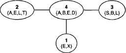
Covering join trees provide the required data structure for the introduction of more general and economical local computation schemes. We now follow the same procedure as in Section 3.5 and assign the knowledgebase factors to covering nodes. This defines an assignment mapping according to the following definition.

Definition 3.9 Let (V, E, λ, D) be a covering join tree for the factorization

A function

is called an assignment mapping for regarding V if for every i {1, …, m} we have d(i) λ(a(i)).

Example 3.15 The assignment mapping of Figure 3.8 is a(1) = 4, a(2) = 4, a(3) = 2, a(4) = 2, a(5) = 3, a(6) = 1, a(7) = 5, a(8) = 2. Observe a/50 that there are in general several possible assignment mappings.

It was already pointed out that some nodes may go away empty-handed from this factor distribution process. Also, it may be that the domain of a factor assigned to a certain node does not fill its node label completely. We therefore initialize every join tree node with the neutral element of its label.

Definition 3.10 Let a be an assignment mapping for a factorization regarding the nodes V of a covering join tree (V, E, λ, D). The factor assigned to node i V is

(3.30)

This assures that for every node factor Ψi we have d(Ψi) = λ(i). However, it will later be shown in Section 3.10 that we may in fact dispose of this artificial filling.

Example 3.16 The join tree of Figure 3.11 is a covering join tree for the factorization of Instance 2.1 (but not for the inference problem since the query is not covered). The corresponding factor domains are given in Example 3.12. A possible factor assignment is: a(1) = a(2) = 1, a(3) = a(4) = a(8) = 3, a(5) = 2, a(6) = 7 and a(7) = 4. No factor is assigned to the nodes 5 and 6. This assignment creates the node factors:

• 
• 
• 
• 
• 
• 
• 

The factors Ψi are usually called join tree factors and correspond either to (the vacuous extension of) a single factor of the original knowledgebase, a combination of multiple factors, or to a neutral element, if the factor set of the combination in equation (3.30) is empty. The following lemma shows that the join tree factors provide an alternative factorization to the knowledgebase of the inference problem:

Lemma 3.8 It holds that

(3.31)

Proof: The assignment mapping assigns every knowledgebase factor to exactly one join tree node. It therefore follows from the commutativity of combination and the neutrality axiom that

The second equality follows from the third requirement of Definition 3.8.

When a covering join tree is obtained from the graphical fusion process, its node numbering is determined by the variable elimination sequence, i.e. a node gets number if is was created during the elimination of the i-th variable in the fusion process. This particular numbering shaped up as very useful to identify the sending and receiving node during the message-passing process. However, if local computation is defined on arbitrary covering join trees, such a node numbering has to be introduced artificially. To do so, we first fix a node which covers the query as root node and assign the number |V| to it. Then, by directing all edges towards the root node m, it is possible to determine a numbering in such a way that if j is a node on the path from node i to m, then j > i. Formally, let (V, E, λ, D) be a join tree. We determine a permutation π of the elements in V such that

• π(k) = |V|, if k is the root node;
• π(j) > π(i) for every node j V lying on the path between i and |V|.

The result is a renumbered join tree (V, E′, λ, D) with edges E′ = {(π(i), π(j)): (i,j) E} that is usually called a directed join tree towards the root node |V|. Note also that such a numbering is not unique. It is furthermore convenient to introduce the notions of parents, child, and leaves with respect to this node numbering:

Definition 3.11 Let (V, E, λ, D) be a directed join tree towards root node |V|.

• The parents pa(i) of a node i are defined by the set
• Nodes without parents are called leaves.
• The child ch(i) of a node i < |V| is the unique node j with j > i and (i, j) E.

In this numbering parents always have a smaller number than their child.

Definition 3.12 Let (V, E, λ, D) be a directed join tree towards root node |V|.

• The separator sep(i) of a node i < |V| is defined by sep(i) = λ(i) λ(ch(i)).
• The eliminator elim(i) of a node i < |V| is defined by elim(i) = λ(i) - sep(i).

Finally, the definition of a tree implies that whenever one of its edges (i, ch(i)) is removed, the tree splits into two separated trees where the one that contains the node i is called subtree rooted to node i, abbreviated by i. Clearly, the running intersection property remains satisfied if join trees are cut in two.

Example 3.17 Consider the join tree of Figure 3.15 which corresponds to the join tree of Figure 3.11 directed towards node {B,D,E} and renumbered according to the above scheme. The parents of node 5 are pa(5) = {2, 4} and its child is ch(5) = 6. Further, we have sep(5) = {E, L} and elim(5) = {B}. Also, if we for example cut the edge between the nodes 5 and 6, we obtain two trees that both satisfy the running intersection property.

3.7 JOIN TREE CONSTRUCTION

Before we actually describe how local computation can be performed on arbitrary covering join trees, we should first say a few words about how to build covering join trees for an inference problem. In fact, this topic is a broad research field by itself, which makes it impossible at this point to give all the important references. However, from our complexity studies of the fusion algorithm, we know the principal quality criterion of a join tree. The treewidth of the join tree determines the complexity of local computation and therefore, we focus on finding covering join trees whose treewidth is as small as possible. We further know that the treewidth of the inference problem provides a lower bound. Finding such an optimum join tree is NP-hard. Thus, if we want to achieve reasonable local computation complexity, we are forced to fall back on heuristics. There are a many different heuristics to find a suitable variable elimination sequence as for example (Rose, 1970; Bertele & Brioschi, 1972; Yannakakis, 1981; Kong, 1986; Almond & Kong, 1991; Haenni & Lehmann, 1999; Allen & Darwiche, 2002; Hopkins & Darwiche, 2002). An overview of recommended heuristics can be found in (Lehmann, 2001; Dechter, 2003) and a comparison is drawn by (Cano & Moral, 1995). These methods deliver a variable elimination sequence from which the covering join tree is constructed using some possibly improved version of the graphical fusion process of Section 3.2.1. The justification of this approach is the fact that no better join tree can be found if we do without variable elimination (Arnborg, 1985; Dechter & Pearl, 1989). However, building a join tree from a previously fixed elimination sequence requires a lot of knowledgebase rearrangement operations that in turn can lead to severe performance problems. A particularly efficient way has been proposed by (Lehmann, 2001) and uses a data-structure called variable-valuation-linked-list. It directly returns a covering join tree including an assignment mapping that assigns at most one knowledgebase factor to each join tree node. This is often a very advantageous property since it avoids that combinations are executed before the actual local computation algorithm is started. On the other hand, such join trees generally contain more nodes and therefore also require to store more factors and messages during local computation. To sum it up, covering join trees can be found by the graphical fusion process and some variable elimination sequence. As a complement, we skim over an alternative but equivalent method to construct join trees starting from the primal graph of the knowledgebase.

3.7.1 Join Tree Construction by Triangulation

Imagine the primal graph representation of a knowledgebase as introduced in Section 2.2. Here, the variables of the knowledgebase valuations correspond to the graph nodes, and two nodes are linked if the corresponding variables occur in the domain of the same valuation. Its associated dual graph has a node for each factor domain, and the nodes are connected if they share a common variable. Therefore, each valuation is naturally covered by some node of the dual graph. Finding a covering join tree therefore consists in removing edges from the dual graph until it is a tree that satisfies the running intersection property. The following theorem (Beeri et al., 1983) states under which condition this is possible:

Theorem 3.4 A graph is triangulated if, and only if, its dual graph has a join tree.

A graph is called triangulated if each of its cycles of four or more nodes has an edge joining two nodes that are not adjacent in the cycle. Elsewhere, triangulated graphs are also called chordal graphs where the chord refers to the introduces edges during the triangulation process. Figure 3.12 shows a cycle of six nodes together with two possible triangulations.

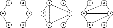
Obviously, there are different possibilities to triangulate a graph. Various algorithmic aspects of this task are discussed in (Tarjan & Yannakakis, 1984). Here, we give a simple procedure from (Cano & Moral, 1995) that is based on a node elimination sequence (X1, …, Xn). Applied to primal graphs, this clearly corresponds to a variable elimination sequence.

• For i = 1, …, n:

• To obtain the triangulation of the original graph, add all edges in ∪u=1n Li.

In fact, this algorithm corresponds exactly to the procedure of constructing an induced graph from a primal graph described in Section 3.2.4. We thus conclude that the induced graph of a primal graph ordered along a given variable elimination sequence is equal to the triangulated graph obtained from the same elimination sequence. This supports the above statement that constructing join trees via graph triangulation is just another interpretation of the methods introduce before.

Example 3.18 Consider the knowledgebase of the medical example from Instance 2.1, whose domains are listed in Example 3.1, and draw up its primal graph:

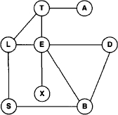
If we want to ensure that the join tree covers some specified query, then the query must also be added to the primal graph. This mirrors the insertion of a corresponding neutral element into the knowledgebase. We choose the elimination sequence (X, S, L, T, E, A, B, D) and execute the above algorithm:

• Elimination of variable X:

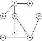
• Elimination of variable S:

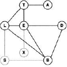
• Elimination of variable L:

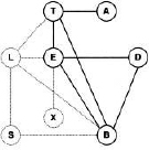
• Elimination of variable T:

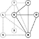
• Elimination of variable E:

At this point, the triangulation process can be stopped because the remaining nodes form a clique. Figure 3.13 shows the completed triangulation of the primal graph which is in fact equal to the induced graph that we obtain from the same elimination sequence by the procedure of Section 3.2.4, see Example 3.8. We further observe that the triangulated graph has the maximal cliques {B, L, S}, {B, E, L, T}, {A, E, T}, {A, B, E, T}, {A, B, D, E} and {E, X}.

We now have a triangulated graph from which we can derive the join tree that was promised in Theorem 3.4. For this purpose, we identify all maximal cliques in the triangulated graph and build a new graph whose nodes are the maximal cliques. Each node is connected to all other nodes and each edge is labeled with the intersection of the corresponding cliques. Such a graph is called a join graph. Further, we refer to the weight of an edge in the join graph as the number of variables in the edge label. The following theorem is proved in (Jensen, 1988).

Theorem 3.5 A spanning tree of a join graph is a join tree if, and only if its sum of edge weights is maximal.

An important advantage of this characterization is that standard enumeration algorithms for spanning trees (Broder & Mayr, 1997) can be used. Note also that several join trees with the same weight may exist, as it can easily be seen in the following example. These join trees clearly have the same nodes and thus the same treewidth, but they may distinguish in the separator widths.

Example 3.19 The left-hand side of Figure 3.14 shows the join graph obtained from the cliques identified in Example 3.18. There are 6 nodes which implies that a spanning tree must have 5 edges. A spanning tree with maximal weight can be found by including the three edges with weight 3 and choosing the other two edges with maximal weight among the remaining candidates. There are several join trees with maximal weight, one being shown on the right-hand side of Figure 3.14.

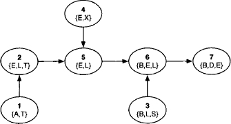
We now abandon the widespread field of join tree construction and focus in the following sections on the solution of single-query inference problems based on a previously built covering join tree.

3.8 THE COLLECT ALGORITHM

The collect algorithm is the principal local computation scheme for the solution of single-query inference problems. It presupposes a covering join tree for the current inference problem that is directed and numbered according to the scheme at the end of Section 3.6 and that keeps a factor Ψj on every node j which is defined according to equation (3.30). We therefore say that Ψj represents the initial content of node j. The collect algorithm can then be described by three simple rules:

R1:	Each node sends a message to its child when it has received all messages from its parents. This implies that leaves (i.e. nodes without parents) can send their messages right away.
R2:	When a node is ready to send, it computes the message by projecting its current content to the separator and sends the message to its child.
R3:	When a node receives a message, it updates its current content by combining it with the incoming message.

This procedure is repeated up to the root node. It follows from this first sketch that the content of the nodes may change during the algorithm’s run. To incorporate this dynamic behavior, the following notation is introduced.

• is the initial content of node j.
• is the content of node j before step i of the collect algorithm.

The particular way of numbering the nodes of the directed join tree implies that at step i, node i can send a message to its child. This allows the following specification of the collect algorithm.

• At step i, node i computes the message

(3.32)

This message is sent to the child node ch(i) with node label λ(ch(i)).

• The receiving node ch(i) combines the message with its node content:

(3.33)

The content of all other nodes does not change at step i, i.e. for all j ≠ ch(i)

(3.34)

The justification of the collect algorithm is formulated by the following theorem. Remember that the root node has been chosen in such a way that it covers the query of the inference problem.

Theorem 3.6 At the end of the collect algorithm, the root node r = |V| contains the marginal of relative to λ(r),

(3.35)

The proof of this theorem can be found in the appendix of this chapter. The marginal can now be used to solve the single-query inference problem by one last projection to the query x, because the latter is covered by the root node.

(3.36)

A summary of the collect algorithm is given in Algorithm 3.3. The input to this algorithm is a covering join tree (V, E, λ, D) where each node i V contains a factor Ψi Φ. Also, the query x is given as input for the final projection of equation (3.36) performed in the statement.

Algorithm 3.3 The Collect Algorithm

The medical inference problem of Instance 2.1 is based on variables which allows us to express projection by variable elimination. Thus, if we illustrate the collect algorithm on the same join tree as the fusion algorithm in Example 3.13, we repeat exactly the same computations. We therefore consider a new query for the illustration of the collect algorithm in Example 3.20.

Example 3.20 We reconsider the knowledgebase of the medical inference problem with the new query × = {B, E} and use the join tree of Figure 3.11 for the computation. It has already been shown in Example 3.16 that this join tree covers our knowledgebase. Since node 4 of Figure 3.11 covers the new query, we directly have a covering join tree for the new inference problem. However, the node numbering has to be modified such that node 4 becomes the new root node. A possible renumbering is shown in Figure 3.15 and the new node factors are: . The messages sent during the collect algorithm are:

• 
• 
• 
• 
• 
• 

At the end of the message-passing, the content of node 7 is:

and, according to Theorem 3.6, the query {B, E} is obtained by one last projection:

3.8.1 The Complexity of the Collect Algorithm

In the complexity study of the fusion algorithm, we brought forward the argument that all computations take place within the nodes of the join tree whose labels bound the domains of all intermediate results. Therefore, the treewidth of the inference problem, which reflects the minimum size of the largest node label over all possible covering join trees, became the decisive complexity factor. This argumentation was based on the interpretation of the fusion algorithm as message-passing scheme on a (particular) covering join tree. Exactly the same statement can also be made for the time complexity of the collect algorithm. However, the decoupling of the join tree construction process from the actual local computation gives us considerably more liberty in choosing an appropriate covering join tree for a given inference problem. One could therefore think that perhaps other methods exist that lead to better join trees than variable elimination can produce. The answer to this question has already been given in Section 3.7 since for a join tree of fixed treewidth, there always exists a variable elimination sequence producing a join tree of equal treewidth (Arnborg, 1985; Dechter & Pearl, 1989). The only difference with respect to the time complexity of fusion given in equation (3.19) is that the number of join tree nodes is no more proportional to the number of variables in the inference problem plus the number of knowledgebase factors. This results from the decoupling of join tree construction from local computation. Thus, recall that each node combines all incoming messages to its content. There are |E| = |V| - 1 edges, hence |V| - 1 combinations to execute. Additionally, each new message is obtained by projecting the current node content to the separator. This adds another |V| - 1 projections which altogether gives 2(|V| - 1) operations. We therefore obtain for the time complexity of the collect algorithm

(3.37)

In the derivation of the time complexity for the fusion algorithm, the number of operations was bounded by m + |d()| with m being the number of knowledgebase factors. It is fairly common for complexity considerations to assume a factor assignment mapping of the collect algorithm that assigns at most one knowledgebase factor to each join tree node. This ensures according to equation (3.30) that no combinations of knowledgebase factors are executed before the collect algorithm is started, since this would clearly falsify the complexity analysis of the latter. Therefore, similar assumptions will also be made for the complexity analysis of all subsequent local computation schemes. We then have m ≤ |V| and since |V| ≈ |d()| in the fusion algorithm, we conclude that both algorithms have the same time complexity.

Also, the space complexity is still similar to the message-passing implementation of the fusion algorithm given in equation (3.29), although the messages are generally much smaller. The reason is that each node combines incoming messages to its node content. Then, the message can be discarded that makes its smaller size irrelevant. Instead, we still keep one factor per node in memory whose size is bounded by the node label. Thus, we end with the following space complexity:

(3.38)

3.8.2 Limitations of the Collect Algorithm

In Section 3.2.6 we addressed two important limitations of the fusion algorithm which should now be discussed from the viewpoint of collect. Collect is entirely based on projection and can therefore be applied to valuations taking domains from an arbitrary lattice. However, in such cases we need more general prerequisites since the definition of a join tree is still based on variables. The concepts generalizing join trees are Markov trees where the notion of conditional independence between elements of a general lattice replaces the running intersection property (Kohlas & Monney, 1995). We therefore conclude that the collect algorithm is, from this point of view, more generally applicable than the fusion algorithm.

The attentive reader may have noticed that we expressed the statement about the generality of the collect algorithm with great care. In fact, the version of the collect algorithm given here can be applied to valuation algebras on general lattices but, on the other hand, requires neutral elements for the initialization of join tree nodes. This in turn is not required for the fusion algorithm, and it is indeed an extremely limiting requirement. We have for example seen in Instance 3.4 that neutral elements in the valuation algebra of relations often correspond to infinite tables which can hardly be used to initialize join tree nodes. Even worse, the valuation algebra of density functions from Instance 3.5 does not provide neutral elements at all. This dependency of the collect algorithm on neutral elements was tacitly accepted for many years. It can, however, be avoided. A general solution that further increases the efficiency of the collect algorithm has been proposed by (Schneuwly et al., 2004). We know from Lemma 3.5 that neutral elements also behave neutral with respect to valuations of larger domains. Thus, the neutral element behaves neutral with respect to all valuations Φ and could therefore be used to initialize join tree nodes. Instead of a neutral element per domain, we only need a single neutral element for the empty domain. Moreover, we will see in the following section that an element with this property can always be adjoined to any valuation algebra, if the latter does not provide neutral elements. This element is called identity element and its use finally leads to a general collect algorithm that can be applied to every valuation algebra without any restriction. A particular implementation of this algorithm will also exempt the message-passing conception from its inefficient space complexity.

3.9 ADJOINING AN IDENTITY ELEMENT

We are going to show in this section that a single identity element can be adjoined to any valuation algebra. This identity element then replaces neutral elements in the generalized version of the collect algorithm presented in Section 3.10. Let be a valuation algebra according to Definition 1.1. We add a new valuation e to Φ and denote the resulting system by . Labeling, combination and projection are extended from Φ to Φ′ in the following way:

If another element e′ with the identical property that for all Φ′ already exists in Φ′, there is no need to perform the extension. This is in particular the case if the valuation algebra provides a neutral element for the empty domain. We will next see that the proposed extension of conserves the properties of a valuation algebra. The simple proof of this lemma is given in (Schneuwly et al., 2004).

Lemma 3.9 with extended operations d′, and is a valuation algebra.

If there is no danger of confusion, we usually identify the operations in with their counterparts in . Doing so, we subsequently write d for d′, for ′ and for .

3.10 THE GENERALIZED COLLECT ALGORITHM

Finally, in this section, we derive the most general local computation scheme for the solution of single-query inference problems. It essentially corresponds to the collect algorithm of Section 3.8 but avoids the use of neutral elements. Instead, we assume a valuation algebra with an identity element e Φ. The first occurrence of neutral elements in the collect algorithm is in equation (3.30) that defines the join tree factorization or, in other words, the initial node content for the message-passing. This equation can easily be rewritten using the identity element:

Definition 3.13 Let a be an assignment mapping for a factorization regarding the nodes V of a covering join tree (V, E, λ, D). The node factor i V assigned by a is

(3.39)

Also, the important statement of Lemma 3.8 still holds under this new setting:

In the subsequent sections, we always consider this modified factorization as join tree factorization. Each factor Ψi corresponds either to a single factor of the original knowledgebase, a combination of some of them, or to the identity element if the factor set of the combination in equation (3.39) is empty. However, there is one essential difference between the two factorizations of equation (3.30) and (3.39). When neutral elements are used, it is always guaranteed that the domain of the factors covers the join tree node label entirely, i.e. we have d(i) = λ(i). This is a consequence of the neutral element used in equation (3.30). On the other hand, if the identity element is used to initialize join tree nodes, we only have d(i) λ(i). It is therefore important to distinguish between the node label λ(i) and the node domain d(i): the node domain refers to the domain of the factor that is actually kept by the current node and this value may grow when incoming messages are combined to the node content. The label, on the other hand, represents the largest possible domain of a factor that would fit into this node and always remains constant.

Example 3.21 The factors of Example 3.16 change only marginally under this modified definition. We now have .

The generalized collect algorithm for the solution of single-query inference problems without neutral elements can now be described by the following rules:

R1:	Each node sends a message to its child when it has received all messages from its parents. This implies that leaves can send their messages right away.
R2:	When a node is ready to send, it computes the message by projecting its current content to the intersection of its domain and its child’s node label.
R3:	When a node receives a message, it updates its current content by combining it with the incoming message.

One has to look closely to detect the difference to the collect algorithm given in Section 3.8. In fact, only Rule 2 changed in a small but important way. Remember, the node domain may now be smaller than the node label due to the use of identity elements. If node i would project its node factor to the separator , then this could lead to an undefined operation since does not necessarily hold anymore. Instead, the factor is projected to . In Section 3.8 we already introduced a notation to incorporate the dynamic behavior of the node factors during the message-passing. This notation must now be extended to take the growing node domains into consideration:

• is the initial content of node j.
• is the content of node j before step i of the collect algorithm.

A similar notation is adopted to refer to the domain of a node:

• is the initial domain of node j.
• is the domain of node j before step i of the collect algorithm.

As before, the particular way of numbering the nodes of the directed join tree implies that at step i, node i can send a message to its child. This allows the following specification of the generalized collect algorithm.

• At step i, node i computes the message

(3.40)

This message is sent to the child node ch(i) with node label λ(ch(i)).

• The receiving node ch(i) combines the message with its node content:

(3.41)

Its node domain changes to:

(3.42)

The content of all other nodes does not change at step i,

(3.43)

for all j ≠ ch(i), and the same holds for the node domains:

(3.44)

The justification of the collect algorithm is formulated in the following theorem. Remember that in case of single-query inference problems, the root node is always chosen in such a way that it covers the query.

Theorem 3.7 At the end of the generalized collect algorithm, the root node r = |V| contains the marginal of relative to λ(r),

(3.45)

The proof of this theorem is given in the appendix of this chapter. We should also direct our attention to the implicit statement of this theorem that the node domain of the root node always corresponds to its node label λ(r) at the end of the collect algorithm. This is again a consequence of the third requirement in Definition 3.8 as shown in the proof of the collect algorithm. We then obtain the solution of the single-query inference problem by one last projection:

(3.46)

Algorithm 3.4 The Generalized Collect Algorithm

Example 3.22 Example 3.21 gives a modified join tree factorization based on the use of identity elements instead of neutral elements. Since this concerns only the two factors Ψ5 and Φ6, only the messages μ5→6 and μ6→7 change with respect to Example 3.20.

5:

6:

The collect algorithm based on identity elements instead of neutral elements is the most general and fundamental local computation scheme for the solution of single-query inference problems. Moreover, this algorithm will play an important part in the following chapter in which local computation procedures for multi-query inference problems are studied. It turns out that many algorithmic insights concerning the computation of multiple queries can be derived from the correctness of the collect algorithm. We therefore list some further properties for later use, starting with a partial result of the generalized collect theorem for each subtree:

Lemma 3.10 At the end of the generalized collect algorithm, node i contains

(3.47)

The proof is given in the appendix of this chapter. Comparing this result with Theorem 3.7 indicates that only the label of the root node is guaranteed to be filled after the generalized collect algorithm, because it is not sure that all the variables in λ(i) are covered by some factors in the current subtree. However, as the following lemma states, the node labels can be scaled down to coincide with the node domain and the resulting tree will again be a join tree.

Lemma 3.11 At the end of the collect algorithm executed on a join tree = (V, E, λ, D), the labeled tree * = (V, E, λ*, D) with

for i = 1, …, r is still a covering join tree for the projection problem.

Proof: It will be shown that the running intersection property is still satisfied between the nodes of the labeled tree *. Let i and j be two nodes whose reduced labels contain X, i.e. . There exists a node k with X λ(k) and i, j ≤ k, since . By the same token, X λ(ch(i)). Then, from

follows that X λ*(ch(i)) and by induction along the path from i to k, X λ*(k). The same argument applies to the nodes on the path from j to k and therefore the running intersection property holds for *. The fact that * covers the original knowledgebase factors follows directly from .

The last property highlights the relationship between node domains and labels:

Lemma 3.12 It holds that

(3.48)

Proof: The left-hand part of this equation is clearly contained in the right-hand part, because . Remembering that for i = 1, …, r and that are non-decreasing in j = 1, 2 … the reversed inclusion is derived as follows:

The last equality follows from .

3.10.1 Discussion of the Generalized Collect Algorithm

The generalized collect algorithm is the most general and fundamental local computation scheme for the solution of single-query inference problems. It depends neither on a particular lattice such as the fusion algorithm, nor on the existence of neutral elements. Consequently, this algorithm can be applied to any valuation algebra and it is therefore also qualified to serve as a starting point for the development of further local computation procedures in the following chapters. Besides its generality, there is a second argument for the use of the generalized collect algorithm. Using neutral elements to initialized join tree nodes blows the node content up until its domain agrees with the node label. All operations performed during the message-passing then take place on this maximum domain. On the other hand, using the identity element keeps the node domains as small as possible with the node label as upper bound. This makes the generalized collect algorithm more efficient, although its general complexity is not affected by this optimization. However, the real benefit of using the generalized collect algorithm becomes apparent when dealing with multi-query inference problems. We therefore refer to Section 4.1.3 in which the discussion about this performance gain is reconsidered and illustrated.

3.10.2 The Complexity of the Generalized Collect Algorithm

We have just mentioned that the use of the identity element instead of neutral elements for the initialization of join tree nodes does not change the overall complexity of the collect algorithm. Computations still take place on the factor domains that are bounded by the largest node label, and incoming messages are still combined to the node content. This repeats the two main arguments that lead to the complexity bounds given in equation (3.37) and (3.38). However, there is a technique to reduce the space complexity of the collect algorithm coming from the Shenoy-Shafer architecture that will be introduced in the following chapter. We first point out that the space requirement of the identity element can be neglected since it has been adjoined to the valuation algebra (Pouly & Kohlas, 2005). If we furthermore stress a factor distribution that assigns at most one knowledgebase factor to each join tree node, the node initialization process does not require any additional memory. This is again in contrast to the use of neutral elements for initialization. We next assume that each node has a separate mailbox for all its parents. Then, instead of combining a message directly to the node content, it is simply stored in the corresponding mailbox of the child node. Once all mailboxes are full, a node computes the message for its child node by combining its still original node content with all the messages of its mailboxes. Clearly, this is equal to the node content just before computing the message μi→ch(i) in the above scheme. Finally, we project this valuation as proposed in equation (3.40) and send the result to the mailbox of the child node. It is clear that the statement of Theorem 3.7 (and Lemma 3.10) must be adapted under this optimization. At the end of the message-passing, the root node does not contain the projection of the objective function to its node label directly, but this result must first be computed by combining its still original node content with all the messages of its mailboxes. We pass on a formal proof for the correctness of this particular implementation of the generalized collect algorithm at this point, since it will be given in Section 4.1.1. Instead, we now analyze its impact on the space complexity: this procedure does not combine messages to the content of the receiving nodes but stores them in mailboxes and computes their combination only as an intermediate result of the message creation process, or to return the final query answer. Then, as soon as the message has been sent, this intermediate result can be discarded. Thus, instead of keeping |V| node factors, we only store |E| = |V| - 1 messages. According to equation (3.40) the size of a message sent from node i to node ch(i) is always bounded by the size of the corresponding separator . Consequently, the space of all messages in a complete run of the collect algorithm are bounded by the largest separator size in the join tree called its separator width. Similarly to the treewidth, we define the separator width of an inference problem by the smallest separator width over all possible covering join trees and write sep* for this measure. This leads to the following bound for the space complexity of this implementation:

(3.49)

We conclude from the definition of the separator that sep* ≤ ω* or, in other words, that the separator width of an inference problem is not larger than its treewidth. Moreover, in practical applications the separator width is often much smaller than the treewidth. This generalizes the space complexity derived from the fusion algorithm in equation (3.20) to arbitrary covering join trees. It will be shown in Section 5.6 that for certain valuation algebras, we can omit the explicit computation of the node content and directly derive the message from the original node factor and the messages in the mailboxes. Then, the first term in the equation (3.49) vanishes, and the mailbox implementation of the generalized collect algorithm indeed provides a noteworthy improvement regarding space complexity.

It corresponds to the relevant literature (Pouly, 2008; Schneuwly, 2007; Schneuwly et al., 2004) to introduce the generalized collect algorithm in the above manner, although the improvement based on mailboxes is clearly preferable for computational purposes. On the other hand, combining messages directly to the node content often simplifies the algebraic reasoning about the collect algorithm and makes it possible to apply its correctness proof to other local computation schemes. In the following chapter, we will introduce the Shenoy-Shafer architecture as a local computation technique to solve multi-query inference problems. This architecture is entirely based on the mailbox scheme, and if we only consider some part of its message-passing, we naturally obtain the mailbox implementation of the generalized collect algorithm. This allows us to refer to equation (3.49) when talking about the space complexity of the generalized collect algorithm. Finally, since the collect algorithm with neutral elements does not have any advantage over its generalized version, we subsequently refer to the second approach as the collect algorithm.

3.11 AN APPLICATION: THE FAST FOURIER TRANSFORM

In this last section, we focus on the application of local computation to the single-query inference problem derived from the discrete Fourier transform in Instance 2.6. There are several reasons why this exact problem has been chosen for a case study: from a historic perspective, local computation methods were introduced to deal with problems of exponential (or even higher) complexity. But a direct computation of the discrete Fourier transform given in equation (2.8) only requires O(N2) operations, if N denotes the number of signal samplings. Moreover, a clever arrangement of the operations even leads to a O(N • log N) complexity known as the fast Fourier transform. In fact, there is a whole family of algorithms that share this improved complexity, such that the notion of a fast Fourier transform does not refer to a single algorithm but rather to all algorithms that solve the discrete Fourier transform with a time complexity of O(N · log N). Our case study thus shows the effect of applying local computation to a polynomial problem.

3.12 The Fast Fourier Transform

Instance 2.6 transformed the discrete Fourier transform into a single-query inference problem by the introduction of variables. The next step therefore consists in finding a covering join tree for the inference problem of equation (2.9). This however is not a difficult task due to the very structured factor domains in the inference problem. This structure is illustrated in Figure 2.11 on page 44. Figure 3.16 shows a possible join tree for the discrete Fourier transform. There are m + 1 nodes, and we quickly remark that the running intersection property is satisfied. It is furthermore a covering join tree: the root node corresponds to the query {K0, …, Km-1} and the knowledgebase factors can be distributed as shown in Figure 3.16. Thus, executing the generalized collect algorithm on this join tree computes a discrete Fourier transform.

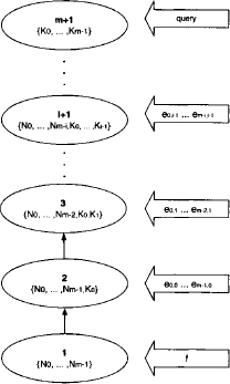
Let us now analyse the time complexity of these computations. It is known from Section 3.10.2 that the time complexity of the generalized collect algorithm is bounded by

We used the valuation algebra of (complex) arithmetic potentials in the derivation of the inference problem for the discrete Fourier transform. All variables are binary and we obtain a possible weight predictor from equation (3.17). Also, we have |V| = m + 1 nodes, and the largest node label has m + 1 variables. This specializes the complexity bound to:

In Instance 2.6 we chose N = 2m, thus m = log N which finally results in

This analysis shows that we obtain the time complexity of the fast Fourier transform by application of local computation. It is important to note that the local computation approach does not correspond to the classical scheme of J. Cooley and J. Tukey (Cooley & Tukey, 1965) that is based on the divide-and-conquer paradigm. Nevertheless, local computation reproduces the same complexity which makes it join the family of fast Fourier transforms. From a more general perspective, this result suggests that there may be good reasons to apply local computation techniques also to polynomial problems. This opens a new field of application for the theory in this book that has not yet been caught completely by the research community. Further applications of local computation to polynomial problems will be studied in Chapter 6 and 9 which both deal with formalism to model path problems in graphs.

3.12 CONCLUSION

This chapter was focused on the solution of single-query inference problems. We pointed out that the memory requirement of valuations as well as the time complexity of their operations generally increase with the size of the involved domains. This increase may be polynomial, but it is in many cases exponential or even worse which makes a direct computation of inference problems impossible. Instead, it is essential that algorithms confine in some way the size of all intermediate results that occur during the computations. This is the exact promise of local computation. The simplest local computation scheme is the fusion or bucket elimination algorithm. It is based on variable elimination instead of projection and is therefore only suitable for valuation algebras based on variable systems. The analysis of its time and space complexity identified the treewidth of the inference problem as the crucial complexity measure for local computation. It also turned out that especially the memory consumption of the fusion algorithm is often too high for practical purposes. A very promising approach to tackle these problems is to decouple join tree construction from the actual local computation process. We may then take an arbitrary covering join tree for the solution of a given inference problem and describe local computation as a message-passing scheme where nodes act as virtual processors that independently compute and transmit messages. Doing so, all local computation schemes become distributed algorithms. The decoupling process leads to the collect algorithm that is based on projection and therefore also applicable for valuations with domains from an arbitrary lattice. In its first occurrence, however, the collect algorithm presupposed the existence of neutral elements to initialize join tree nodes. In addition, it suffered from an even worse space complexity than the fusion algorithm. An algebraic solution for the dependence on neutral elements adjoins a unique identity element to the valuation algebra that is henceforth used for node initialization. Now, the collect algorithm can be applied to all formalisms that satisfy the valuation algebra axioms without any kind of restriction. Furthermore, computations generally take place on smaller domains and no unnecessary combinations with neutral elements are executed. The last addressed issue was the still unsatisfactory space complexity of the collect algorithm that comes from the algebraic description where each node combines incoming messages to its content. Alternatively, we proposed an implementation where messages are stored in mailboxes and only combined for the creation of the child message. Immediately after, the combination is again discarded. Consequently, the collect algorithm only stores messages that generally are much smaller than their combination as node content. The general space complexity reduces slightly under this setting, but for the valuation algebras we are going to study in Chapter 5, this reduction may be considerable. A similar caching policy based on mailboxes will take center stage in the following chapter where multi-query inference problems are treated. The last section of this chapter applied the collect algorithm to the inference problem of a discrete Fourier transform. Doing so, the treewidth complexity of local computation turns into the low polynomial complexity of the fast Fourier transform. This is a strong argument for our claim that local computation may also be useful to solve problems of polynomial nature.

Appendix: Proof of the Generalized Collect Algorithm

We prove Theorem 3.7 which is a generalization of Theorem 3.6. The following lemma will be useful for this undertaking:

Lemma C.13 Define

(C.1)

Then, for i = 1, …, r - 1,

(C.2)

Proof: First, it has to be ensured that yi+1 yi holds in order to guarantee that the projection in equation (C.2) is well denned:

From equation (3.42) it follows that

(C.3)

and since holds.

Next, the following property will be proved:

(C.4)

Assume first that . Then, equation (C.3) implies that and hence, by the definition of yi+1, we have X yi+1. Thus, . On the other hand, assume that . Then, by the running intersection property and the definition of yi+1, X λ(ch(i)) and therefore .

An immediate consequence of equation (3.42) and (3.43) is that

We therefore obtain by application of the combination axiom and Property (C.4):

This proves the first equality of (C.2). The second is shown by induction over i. For i = 1, the equation is satisfied since

Let us assume that the equation holds for i,

Then, by transitivity of marginalization,

which proves (C.2) for all i.

Theorem 3.7 can now be verified:

Proof of Theorem 3.7

Proof: By application of equation (C.2) for i = r - 1, it follows that

(C.5)

It remains to prove that . For this purpose, it is sufficient to show that if X λ(r) then since . Let X λ(r). Then, according to the definition of the covering join tree for an inference problem, there exists a factor Ψj with X d(Ψj). Ψj is assigned to node p = a(j) and therefore . equation (3.41) implies that and follows by repeating this argument up to the root node r.

Proof of Lemma 3.10

Proof: Node i is the root of the subtree i and contains the marginal to of the factors associated with i due to equation (C.5).

PROBLEM SETS AND EXERCISES

C.1 * Propose a weight predictor for the valuation algebra of Gaussian potentials.

C.2 * Exercise B. 1 in Chapter 2 asked to analyse the two inference problems from the discrete cosine transform and the inference problems from the discrete Fourier transform. Continue this analysis by showing that all three problems can be solved with the same covering join tree from Instance 3.12.

C.3 * Apply the collect algorithm to the inference problem of the Hadamard transform derived in Instance 2.5 and show that a clever choice of the covering join tree leads to the time complexity of the fast Hadamard transform. Indications are given in (Aji & McEliece, 2000; Gonzalez & Woods, 2006).

C.4 * If neutral elements are present in a valuation algebra , we may introduce an operation of vacuous extension as shown in equation (3.24). Prove the following properties of vacuous extension:

The solution to this exercise is given in (Kohlas, 2003), Lemma 3.1.

C.5 * In a valuation algebra with neutral element we may define a transport operation as follows: For Φ with d() = x and y D,

(C.6)

Due to Property 8 in Exercise C.4 we also have

(C.7)

Prove the following properties of the transport operation:

The solution to this exercise is given in (Kohlas, 2003), Lemma 3.2.

C.6 * Let be a stable valuation algebra according to Definition 3.6. Based on the transport operation of equation (C.6), we further define the following relation:

For , Ψ Φ with d() = x and d(Ψ) = y we have

(C.8)

C.7 ** Let be a stable valuation algebra with the congruence relation of equation (C.8). We next consider the induced equivalence classes defined for Φ with d() = x by [] = { Φ: Ψ→x ≡ }. Intuitively, this groups valuations that express the same information, even if they have different domains. As a consequence of equation (C.9) all valuations of the same equivalence class are equal, if they are vacuously extended to the complete variable universe. The elements [] are therefore called domain-free valuations. The set of all equivalence classes forms an algebra Ψ, D, called quotient algebra, with

Since the relation is a congruence, we may define the following operations in :

These operations are well-defined since they do not depend on the chosen representative for the equivalence classes. Verify the following properties in :

The solution to this exercise is given in (Kohlas, 2003), Theorem 3.5. Structures like are called domain-free valuation algebras and posses a rich theory which takes center stage in algebraic information theory.

C.8 ** We have seen in Exercise C.7 that a domain-free valuation algebra can be obtained for every stable valuation algebra. Here, we propose the converse direction to derive a valuation algebra starting from a domain-free valuation algebra. Let r be a set of variables and D = P(r) its powerset lattice. We assume an arbitrary domain-free valuation algebra defined by two operations

satisfying the following axioms:

(D1) Semigroup: Ψ is associative and commutative under combination. There is a neutral element e Ψ such that e ψ = ψ e = ψ for all ψ Ψ.

(D2) Transitivity: For ψ Ψ and x, y D,

(D3) Combination: For ψ, Ψ and x D

(D4) Neutrality: For x D,

(D5) Support: For ψ Ψ,

If for ψ Ψ and x D we have then x is called a support of ψ. Due to Axiom (D5), r is a support of every valuation algebra and, according to (D4), every domain is a support of the neutral element. We next consider the set of pairs

(C.10)

These pairs can be considered as valuations labeled by their supports. Therefore, we define the following operations on :

Prove that together with these operations satisfy the axioms of a stable valuation algebra. Indications can be found in (Kohlas, 2003), Section 3.2. Putting these things together, we may start from a stable valuation algebra and derive a domain-free valuation algebra, from which we may again derive a stable valuation algebra. This last algebra is isomorph to the valuation algebra at the beginning of the process as shown in (Kohlas, 2003). Conversely, we may start from a domain-free valuation algebra, derive a stable valuation algebra and then again a domain-free valuation algebra. Again, the algebras at the beginning and end of this process are isomorph.