CHAPTER 4

COMPUTING MULTIPLE QUERIES

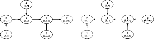
The foregoing chapter introduced three local computation algorithms for the solution of single-query inference problems, among which the generalized collect algorithm was shown to be the most universal and efficient scheme. We therefore take this algorithm as the starting point for our study of the second class of local computation procedures that solve multi-query inference problems. Clearly, the most simple approach to compute multiple queries is to execute the collect algorithm repeatedly for each query. Since we already gave a general definition of a covering join tree that takes an arbitrary number of queries into account, it is not necessary to take a new join tree for the answering of a second query on the same knowledgebase. Instead, we redirect and renumber the join tree in such a way that its root node covers the current query and execute the collect algorithm. This procedure is repeated for each query. In Figure 3.15, arrows indicate the direction of the message-passing for a particular root node and therefore reflect the restrictions imposed on the node numbering. It is easy to see that changing the root node only affects the arrows between the old and the new root node. This is shown in Figure 4.1 where we also observe that a valid node numbering for the redirected join tree is obtained by inverting the numbering on the path between the old and the new root node. Hence, it is possible to solve a multi-query inference problem by repeated execution of the collect algorithm on the same join tree with only a small preparation between two consecutive runs. Neither the join tree nor its factorization have to be modified.

During a single run of the collect algorithm on a covering join tree (V, E, λ, D), exactly |E| messages are computed and transmitted. Consequently, if a multi-query inference problem with n queries is solved by repeated application of collect on the same join tree, n|E| messages are computed and exchanged. It will be illustrated in a short while that most of these messages are identical and their computation can therefore be avoided by an appropriate caching policy. The arising algorithm is called Shenoy-Shafer architecture and will be presented in Section 4.1. It reduces the number of computed messages to 2|E| for an arbitrary number of queries. However, the drawback of this approach is that all messages have to be stored until the end of the total message-passing. This was the main reason for the development of more sophisticated algorithms that aim at a shorter lifetime of messages. These algorithms are called Lauritzen-Spiegelhalter architecture, HUGIN architecture and idempotent architecture and will be introduced in Section 4.3 to Section 4.5. But these alternative architectures require more structure in the underlying valuation algebra and are therefore less generally applicable than the Shenoy-Shafer architecture. More concretely, they presuppose some concept of division that will be defined in Section 4.2. Essentially, there are three requirements for introducing a division operator, namely either separativity, regularity or idempotency. These considerations require more profound algebraic insights that are not necessary for the understanding of division-based local computation algorithms. We therefore delay their discussion to the appendix of this chapter. A particular application of division in the context of valuation algebras is scaling or normalization. If, for example, we want to interpret arithmetic potentials from Instance 1.3 as discrete probability distributions, or set potentials from Instance 1.4 as Dempster-Shafer belief functions, normalization becomes an important issue. Based on the division operator, scaling or normalization can be introduced on a generic, algebraic level as explored in Section 4.7. Moreover, it is then also required that the solution of inference problems gives scaled results. We therefore focus in Section 4.8 on how the local computation architectures of this chapter can be adapted to deliver scaled results directly.

4.1 THE SHENOY-SHAFER ARCHITECTURE

The initial situation for the Shenoy-Shafer architecture and all other local computation schemes of this chapter is a covering join tree for the multi-query inference problem according to Definition 3.8. Join tree nodes are initialized using the identity element, and the knowledgebase factors are combined to covering nodes as specified by equation (3.39). Further, we shall see that local computation algorithms for the solution of multi-query inference problems exchange messages in both directions of the edges. It is therefore no longer necessary to direct join trees. Let us now reconsider the above idea of executing the collect algorithm repeatedly for each query on the same join tree. Since only the path from the old to the new root node changes between two consecutive runs, only the messages of these region are affected. All other messages do not change but are nevertheless recomputed.

Example 4.1 Assume that the collect algorithm has been executed on the left-hand join tree of Figure 4.1. Then, the root node is changed and collect is restarted for the right-hand join tree. It is easy to see that the messages and already existed in the first run of the collect algorithm. Only the node numbering changed but not their content.

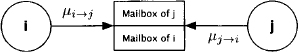
A technique to benefit from already computed messages is to store them for later reuse. The Shenoy-Shafer architecture (Shenoy & Shafer, 1990) organises this caching by installing mailboxes between neighboring nodes which store the exchanged messages. In fact, this is similar to the technique applied in Section 3.10.2 to improve the space complexity of the collect algorithm. This time however, we assume two mailboxes between every pair of neighboring nodes since messages are sent in both directions. Figure 4.2 schematically illustrates this concept.

Then, the Shenoy-Shafer algorithm can be described by the following rules:

R1:	Node i sends a message to its neighbor j as soon as it has received all messages from its other neighbors. Leaves can send their messages right away.
R2:	When node i is ready to send a message to neighbor j, it combines its initial node content with all messages from all other neighbors. The message is computed by projecting this result to the intersection of the result’s domain and the receiving neighbor’s node label.

The algorithm stops when every node has received all messages from its neighbors. In order to specify this algorithm formally, a new notation is introduced that determines the domain of the valuation described in Rule 2. If i and j are neighbors, the domain of node i at the time where it sends a message to j is given by

(4.1)

where d(i) = ωi is the domain of the node content of node i.

• The message sent from node i to node j is

(4.2)

Theorem 4.1 At the end of the message-passing in the Shenoy-Shafer architecture, node i can compute

(4.3)

Proof: The important point is that the messages do not depend on the actual schedule used to compute them. Due to this fact, any node can be selected as root node. Then, the edges are directed towards this root and the nodes are renumbered. The message-passing towards the root corresponds to the collect algorithm and the proposition for node i follows from Theorem 3.7.

Answering the queries of the inference problem from this last result demands one additional projection per query. Since each query xi is covered by some node , we obtain the answer for this query by computing:

(4.4)

Example 4.2 We execute the Shenoy-Shafer architecture on the join tree of Figure 4.3. There are 6 edges, thus 12 messages to be sent and stored in mailboxes. These messages are:

• 
• 
• 
• 
• 
• 
• 
• 
• 
• 
• 
• 

At then end of the message-passing, the nodes compute:

• 
• 
• 
• 
• 
• 
• 

Since the Shenoy-Shafer architecture accepts arbitrary valuation algebras, we may in particular apply it to formalisms based on variable elimination. This specialization is sometimes called cluster-tree elimination. In this context, a cluster refers to a join tree node together with the knowledgebase factors that are assigned to it. Further, we could use the join tree from the graphical representation of the fusion algorithm if we are, for example, only interested in queries that consist of single variables. Under this even more restrictive setting, the Shenoy-Shafer architecture is also called bucket-tree elimination (Kask et al., 2001). Answering more general queries with the bucket-tree elimination algorithm is again possible if neutral elements are present. However, we continue to focus our studies on the more general and efficient version of the Shenoy-Shafer architecture introduced above.

4.1.1 Collect & Distribute Phase

For a previously fixed node numbering, Theorem 4.1 implies that

(4.5)

This shows that the collect algorithm is extended by a single message coming from the child node in order to obtain the Shenoy-Shafer architecture. In fact, it is always possible to schedule a first part of the messages in such a way that their sequence corresponds to the execution of the collect algorithm. The root node will then be the first node which has received the messages of all its neighbors. It suggests itself to name this first phase of the Shenoy-Shafer architecture collect phase or inward phase since the messages are propagated from the leaves towards the root node. It furthermore holds that

for this particular scheduling. This finally delivers the proof of correctness for the particular implementation proposed in Section 3.10.2 to improve the space complexity of the collect algorithm. In fact, the collect phase of the Shenoy-Shafer architecture behaves exactly in this way. Messages are no more combined to the node content but stored in mailboxes, and the combination is only computed to obtain the message for the child node. Then, the result is again discarded, which guarantees the lower space complexity of equation (3.49). The messages that remain to be sent after the collect phase of the Shenoy-Shafer architecture constitute the distribute phase. Clearly, the root node will be the only node that may initiate this phase since it possesses all necessary messages after the collect phase. Next, the parents of the root node will be able to send their messages and this propagation continues until the leaves are reached. In fact, nodes can send their messages in the inverse order of their numbering. Therefore, the distribute phase is also called outward phase.

Lemma 4.1 It holds that

(4.6)

Proof: We have

The second equality follows from equation (4.5).

The next lemma states that the eliminator (see Definition 3.12) of each node will be filled after the collect phase:

Lemma 4.2 It holds that

(4.7)

Proof: Assume X contained in the right-hand part of the equation. Thus, but X . From equation (4.6) can be deduced that . Since

. This proves that

Assume that X is contained in the left-hand part. So, X but which in turn implies that and consequently . Thus, and equality must hold.

The particular scheduling into a collect and distribute phase allows us to describe the intrinsically distributed Shenoy-Shafer architecture by a sequential algorithm. First, Algorithm 4.1 performs the complete message-passing. It does not return any value but ensures that all and are stored in the corresponding mailboxes. To answer a query we then call Algorithm 4.2 which presupposes that the query is covered by some node in the join tree. The message-passing procedure can therefore be seen as a preparation step to the actual query answering.

Algorithm 4.1 Shenoy-Shafer Architecture: Message-Passing

Algorithm 4.2 Shenoy-Shafer Architecture: Query Answering

The implementation of Algorithm 4.2 corresponds to Theorem 4.1, but can easily be changed using equation (4.5). The combination of the node content with all parent messages has already been computed for the creation of the child message in the collect phase. If this partial result is still available, it is sufficient to combine it with the message obtained from the child node. Doing so, Algorithm 4.2 executes at most one combination. Clearly, under this modification, the collect phase becomes again equal to the original description of the collect algorithm in Section 3.10 since we again store the combination of the parent messages with the original node content for each node. This saves a lot of redundant computation time in the query-answering procedure since the combination of the original node factor with all arrived messages is already available, for the prize of an additional factor per node whose space is again bounded by the node label. Hence, we generally refer to such a situation as a space-far-time trade. As memory seems to be the more sensitive resource in many practical applications, it always depends on the context if a space-for-time trade is also a good deal. In the following, we discuss some further optimization issues.

4.1.2 The Binary Shenoy-Shafer Architecture

In a binary join tree, each node has at most three neighbors or, if we reconsider directed join trees, at most two parents. (Shenoy, 1997) remarked that binary join trees generally allow better performance for the Shenoy-Shafer architecture. The reason is that nodes with more than three neighbors compute a lot of redundant combinations. Figure 4.4 shows a non-binary join tree that covers the same knowledgebase factors and queries as the join tree of Figure 4.3. Further, this join tree has one node less such that only 10 messages instead of 12 are sent during the Shenoy-Shafer architecture. We list the messages sent by node 5:

It is easy to see that some combinations of messages must be computed more than once. For comparison, let us also list the messages sent by node 5 in Figure 4.3 that only has three neighbors. Here, no combination is computed more than once:

A second reason for dismissing non-binary join trees is that some computations may take place on larger domains than actually necessary. Comparing the two join trees in Figure 4.5, we observe that the treewidth of the binary join tree is smaller which naturally leads to a better time complexity. On the other hand, the binary join tree contains more nodes that again increases the space requirement. But this increase is only linear since the node separators will not grow. It is therefore generally a good idea to use binary join trees for the Shenoy-Shafer architecture. Finally, we state that any join tree can be transformed into a binary join tree by adding a sufficient number of new nodes. A corresponding join tree binarization algorithm is given in (Lehmann, 2001). Further ways to improve the performance of local computation architectures by aiming to cut down on messages during the propagation are proposed by (Schmidt & Shenoy, 1998) and (Haenni, 2004).

4.1.3 Performance Gains due to the Identity Element

It was foreshadowed multiple times in the context of the generalized collect algorithm that initializing join tree nodes with the identity element instead of neutral elements also increases the efficiency of local computation. In fact, the improvement is absolute and concerns both time and space resources. This effect also occurs when dealing with multiple queries. To solve a multi-query inference problem, we first ensure that each query is covered by some node in the join tree. In most cases, however, queries are very different from the knowledgebase factor domains. Therefore, their covering nodes often still contain the identity element after the knowledgebase factor distribution. In such cases, the performance gain caused by the identity element becomes important. Let us reconsider the knowledgebase of the medical example from Instance 2.1 and assume the query set {{A, B, S, T}, {D, S, X}}. We solve this multi-query inference problem using the Shenoy-Shafer architecture and first build a join tree that covers the eight knowledgebase factors and the two queries. Further, we want to ensure that all computations take place during the run of the Shenoy-Shafer architecture, which requires that each join tree node holds at most one knowledgebase factor. Otherwise, a non-trivial combination would be executed prior to the Shenoy-Shafer architecture as a result of equation (3.39). A binary join tree that fulfills all these requirements is shown in Figure 4.6. Each colored node holds one of the eight knowledgebase factors, and the other (white) nodes store the identity element. We observe that the domain of each factor directly corresponds to the corresponding node label in this particular example.

We now execute the collect phase of the Shenoy-Shafer architecture and send messages towards node 14. In doing so, we are not interested in the actual value of the messages but only in the domain size of the total combination in equation (4.2) before the projection is computed. Since domains are bounded by the node labels, we color each node where the total label has been reached. The result of this process is shown in Figure 4.7. Interestingly, only two further nodes compute on their maximum domain size. All others process valuations with smaller domains. For example, the message sent by node 11 consists of its node content (i.e. the identity element), the message from node 1 (i.e. a valuation with domain {A}) and the message from node 2 (i.e. a valuation of domain {A, T}). Combining these three factors leads to a valuation of domain {A, T} {A, B, S, T}. Therefore, this node remains uncolored in Figure 4.7. If alternatively neutral elements were used for initialization, each node content would be blown up to the label size, or, in other words, all nodes would be colored.

4.1.4 Complexity of the Shenoy-Shafer Architecture

The particular message scheduling that separates the Shenoy-Shafer architecture into a collect and a distribute phase suggests that executing the message-passing in the Shenoy-Shafer architecture doubles the effort of the (improved) collect algorithm. We may therefore conclude that the Shenoy-Shafer architecture adopts a similar time and space complexity as the collect algorithm in Section 3.10.2. There are 2|E| = 2(|V|| - 1) messages exchanged in the Shenoy-Shafer architecture. Each message requires one projection and consists of the combination of the original node content with all messages obtained from all other neighbors. This sums up to |ne(i)| - 1 combinations for each message. Clearly, the number of neighbors is always bounded by the degree of the join tree, i.e. we have |ne(i)| - 1 ≤ deg - 1. In total, the number of operations executed in the message-passing of the Shenoy-Shafer architecture is therefore bounded by

Thus, we obtain the following time complexity bound for the message-passing:

(4.8)

It is clear that we additionally require |ne(i)| - 1 ≤ deg combinations and one projection to obtain the answer for a given query after the message-passing. But since every query must be covered by some node in the join tree, it is reasonable to bound the number of queries by the number of join tree nodes. The additional effort for query answering does therefore not change the above time complexity. Note also that the factor deg is a constant when dealing with binary join trees and disappears from equation (4.8), possibly at the expense of a higher number of nodes.

Regarding space complexity, we recall that the number of messages sent in the Shenoy-Shafer architecture equals two times the number of messages in the improved collect algorithm. Therefore, both algorithms have the same space complexity

(4.9)

4.1.5 Discussion of the Shenoy-Shafer Architecture

Regarding time complexity, the improvement brought by the Shenoy-Shafer architecture compared to the repeated application of the collect algorithm as proposed in the introduction of this chapter is obvious. If we compute projections to all node labels in the join tree, we need |V| executions of the collect algorithm, which result in an overall complexity of

Since the degree of a join tree is generally much smaller than its number of nodes, the Shenoy-Shafer architecture provides a considerable speedup. Both approaches further share the same asymptotic space complexity.

The Shenoy-Shafer architecture is the most general local computation scheme for the solution of multi-query inference problems since it can be applied to arbitrary valuation algebras without restrictions of any kind. Further, it provides the best possible asymptotic space complexity one can expect for a local computation procedure. Concerning the time complexity, further architectures for the solution of multi-query inference problems have been proposed that eliminate the degree from equation (4.8), even if the join tree is not binary. However, it was shown in (Lepar & Shenoy, 1998) that the runtime gain of these architectures compared to the binary Shenoy-Shafer architecture is often insignificant. Moreover, these alternative architectures generally have a worse space complexity, which recommends the application of the Shenoy-Shafer architecture whenever memory is the more problematic resource. On the other hand, the computation of messages becomes much easier in these architectures, and they also provide more efficient methods for query answering.

4.1.6 The Super-Cluster Architecture

A possible improvement that applies to the Shenoy-Shafer architecture consists in a time-for-space trade called super-cluster scheme or, if applied to variable systems, super-bucket scheme (Dechter, 2006; Kask et al., 2001). If we recall that the space complexity of the Shenoy-Shafer architecture is determined by the largest separator in the join tree, we may simply merge those neighboring nodes that have a large separator in-between. Doing so, the node labels grow but large separators disappear as shown in Example 4.3. Clearly, it is again subject to the concrete complexity predictors f and g if this time-for-space trade is also a good deal.

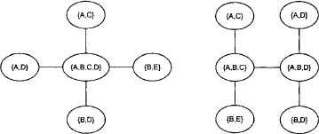
Example 4.3 The join tree shown on the left-hand side of Figure 4.8 has treewidth 5 and separator width 3. The separators are shown as edge labels. The largest separator {B,C, D} is between node 2 and 4. Merging the two nodes leads to the join tree on the right-hand side of this of Figure 4.8. Now, the treewidth became 6 but the separator width is only 2.

The subsequent studies of alternative local computation schemes are essentially based on the assumption that time is the more sensitive resource. These additional architectures then simplify the message-passing by exploiting a division operator in the underlying valuation algebra which therefore requires more algebraic structure. The background for the existence of a division operation will next be examined.

4.2 VALUATION ALGEBRAS WITH INVERSE ELEMENTS

A particular important class of valuation algebras are those that contain an inverse element for every valuation . Hence, these valuation algebras posses the notion of division, which will later be exploited for a more efficient message caching policy during local computation. Let us first give a formal definition of inverse elements in a valuation algebra (Φ, D), based on the corresponding notion in semigroup theory.

Definition 4.1 Valuations are called inverses, if

(4.10)

We directly conclude from this definition that inverses necessarily have the same domain since the first condition implies that and from the second we obtain . Therefore, must hold. It is furthermore suggested that inverse elements are not necessarily unique.

In Appendix D.1 of this chapter, we are going to study under which conditions valuation algebras provide inverse elements. In fact, the pure existence of inverse elements according to the above definition is not yet sufficient for the introduction of division-based local computation architectures since it only imposes a condition of combination but not on projection. For this purpose, (Kohlas, 2003) distinguishes three stronger algebraic properties that all imply the existence of inverses. Separativity is the weakest requirement among them. It allows the valuation algebra to be embedded into a union of groups that naturally include inverse elements. However, the price we pay is that full projection gets lost in the embedding algebra (see Appendix A.3 of Chapter 1 for valuation algebras with partial projection). Alternatively, regularity is a stronger condition than separativity and allows the valuation algebra to be decomposed into groups directly such that full projection is conserved. Finally, if the third and strongest requirement called idempotency holds, every valuation turns out to be the inverse of itself. The algebraic study of division demands notions from semigroup theory, although the understanding of these semigroup constructions is not absolutely necessary, neither for computational purposes nor to retrace concrete examples of valuation algebras with inverses. We continue with a first example of a (regular) valuation algebra that provides inverse elements. Many further instances with division can be found in the appendix of this chapter.

4.1 Inverse Arithmetic Potentials

The valuation algebra of arithmetic potentials provides inverse elements. For with d(p) = s and x we define

It is easy to see that p and p−1 satisfy equation (4.10) and therefore are inverses. In fact, we learn in the appendix of this chapter that arithmetic potentials form a regular valuation algebra.

Idempotency is a very strong and important algebraic condition under which each valuation becomes the inverse of itself. Thus, division becomes trivial in the case of an idempotent valuation algebra. Idempotency can be seen as a particular form of regularity, but it also has an interest in itself. There is a special local computation architecture discussed in Section 4.5 that applies only to idempotent valuation algebras but not to formalisms with a weaker notion of division. Finally, idempotent valuation algebras have many interesting properties that become important in later sections.

4.2.1 Idempotent Valuation Algebras

The property of idempotency is defined as follows:

Definition 4.2 A valuation algebra (Φ, D) is called idempotent if for all and t , it holds that

(4.11)

In particular, it follows from this definition that Thus, choosing Ω = satisfies the requirement for inverses in equation (4.10) which means that each element becomes the inverse of itself. Comparing the two definitions 4.1 and 4.2, we remark that the latter also includes a statement about projection, which makes it considerably stronger. A similar condition will occur in the definition of separativity and regularity given in the appendix of this chapter that finally enables division-based local computation.

Lemma 4.3 The neutrality axiom (A7) always holds in a stable and idempotent valuation algebra.

Proof: From stability and idempotency we derive

Then, by the labeling axiom and the definition of neutral elements,

which proves the neutrality axiom.

4.2 Indicator Functions and Idempotency

The valuation algebra of indicator functions is idempotent. Indeed, for i with and we have

This holds because

4.3 Relations and Idempotency

Is is not surprising that also the valuation algebra of relations is idempotent. For with d(R) = s and we have

Besides their computational importance addressed in this book, idempotent valuation algebras are fundamental in algebraic information theory. An idempotent valuation algebra with neutral and null elements is called information algebra (Kohlas, 2003) and allows the introduction of a partial order between valuations to express that some knowledge pieces are more informative than others. This establishes the basis of an algebraic theory of information that is treated exhaustively in (Kohlas, 2003). See also Exercise D.4 at the end of this chapter.

Definition 4.3 An idempotent valuation algebra with neutral and null elements is called information algebra.

We now focus on local computation schemes which exploit division to improve the message scheduling and time complexity of the Shenoy-Shafer architecture.

4.3 THE LAURITZEN-SPIEGELHALTER ARCHITECTURE

The Shenoy-Shafer architecture answers multi-query inference problems on any valuation algebra and therefore represents the most general local computation scheme. Alternatively, research in the field of Bayesian networks has led to another architecture called the Lauritzen-Spiegelhalter architecture (Lauritzen & Spiegelhalter, 1988), which can be applied if the valuation algebra provides a division operator. Thus, the starting point of this section is a multi-query inference problem with factors taken from a separative valuation algebra. As explained above, separativity is the weakest algebraic condition that allows the introduction of a division operator in the valuation algebra. Essentially, a separative valuation algebra can be embedded into a union of groups Φ*, D where each element of Φ* has a well-defined inverse. On the other hand, it is shown in Appendix D.1.1 that projection is only partially defined in this embedding. We therefore need to impose a further condition on the inference problem to avoid non-defined projections during the local computation process. The knowledgebase factors {1, …, n} may be elements of Φ* but the objective function must be element of Φ which guarantees that can be projected to any possible query. The same additional constraint is also assumed for the HUGIN architecture (Jensen et al., 1990) of Section 4.4.

Remember, the inward phase of the Shenoy-Shafer architecture is almost equal to the collect algorithm with the only difference that incoming messages are not combined with the node content but kept in mailboxes. This is indispensable for the correctness of the Shenoy-Shafer architecture since otherwise, node i would get back its own message sent during the inward phase as part of the message obtained in the outward phase. In other words, some knowledge would be considered twice in every node, and this would falsify the final result. In case of a division operation, we can divide this doubly treated message out, and this idea is exploited by the Lauritzen-Spiegelhalter architecture and by the HUGIN architecture.

The Lauritzen-Spiegelhalter architecture starts executing the collect algorithm towards root node m. We define by Ψ′ the content of node i just before sending its message to the child node. According to Section 3.10 we have

(4.12)

Then, the message for the child node ch(i) is computed as

This is the point where division comes into play. As soon as node i has sent its message, it divides the message out of its own content:

(4.13)

This is repeated up to the root node. Thereupon, the outward propagation proceeds in a similar way. A node sends a message to all its parents when it has received a message from its child. In contrast, however, no division is performed during the outward phase. So, if node j is ready to send a message towards i and its current content is , the message is

which is combined directly with the content of the receiving node i.

Theorem 4.2 At the end of the Lauritzen-Spiegelhalter architecture, node i contains provided that all messages during an execution of the Shenoy-Shafer architecture can be computed.

The proof of this theorem is given in Appendix D.2.1. It is important to note that the correctness of the Lauritzen-Spiegelhalter architecture is conditioned on the existence of the messages in the Shenoy-Shafer architecture, since the computations take place in the separative embedding Φ* where projection is only partially defined. However, (Schneuwly, 2007) weakens this requirement by proving that the existence of the inward messages is in fact sufficient to make the Shenoy-Shafer architecture and therefore also the Lauritzen-Spiegelhalter architecture work. Furthermore, in case of a regular valuation algebra, all factors are elements of Φ and consequently all projections exist. Theorem 4.2 can therefore be simplified by dropping this assumption. A further interesting issue with respect to this theorem concerns the messages sent in the distribute phase. Namely, we may directly conclude that

(4.14)

We again summarize this local computation scheme in the shape of a pseudo-code algorithm. As in the Shenoy-Shafer architecture, we separate the message-passing procedure from the actual query answering process.

Algorithm 4.3 Lauritzen-Spiegelhalter Architecture: Message-Passing

Algorithm 4.4 Lauritzen-Spiegelhalter Architecture: Query Answering

We next illustrate the Lauritzen-Spiegelhalter architecture using the medical knowledgebase. In Instance 2.1 we expressed the conditional probability tables of the Bayesian network that underlies this example in the formalism of arithmetic potentials. It is known from Instance 4.1 that arithmetic potentials form a regular valuation algebra. We are therefore not only allowed to apply this architecture, but we do not even need to care about the existence of messages as explained before.

Example 4.4 Reconsider the covering join tree for the medical knowledgebase of Figure 3.15. During the collect phase, the Lauritzen-Spiegelhalter sends exactly the same messages as the generalized collect algorithm. These messages are given in the Examples 3.20 and 3.22. Whenever a node has sent a message, it divides the latter out of its node content. Thus, the join tree nodes hold the following factors at the end of the inward phase:

• 
• 
• 
• 
• 
• 
• 

The root node does not perform a division since there is no message to divide out. As a consequence of the collect algorithm, it holds that

We then enter the distribute phase and send messages from the root down to the leaves. These messages are always combined to the node content of the receiver:

• Node 6 obtains the message
  
  and updates its node content to
  
  The second equality follows from the combination axiom. For the remaining nodes, we only give the messages that are obtained in the distribute phase.
• Node 5 obtains the message
  
• Node 4 obtains the message
  
• Node 3 obtains the message
  
• Node 2 obtains the message
  
• Node 1 obtains the message
  

At the end of the message-passing, each node directly contains the projection of the objective function to its own node label. This example is well suited to once more highlight the idea of division. Consider node 4 of Figure 3.15: During the collect phase, it sends a message to node 5 that consists of its initial node content. Later, in the distribute phase, it receives a message that consists of the relevant information from all nodes in the join tree, including its own content sent during the collect phase. It is therefore necessary that this particular piece of information has been divided out since otherwise, it would be considered twice in the final result. Dealing with arithmetic potentials, the reader may easily convince himself that combining a potential with itself leads to a different result.

4.3.1 Complexity of the Lauritzen-Spiegelhalter Architecture

The collect phase of the Lauritzen-Spiegelhalter architecture is almost identical to the unimproved collect algorithm. In a nutshell, there are |V| - 1 transmitted messages and each message is combined to the content of the receiving node. Further, one projection is required to obtain a message that altogether gives 2(|V| - 1) operations. In addition to the collect algorithm, the collect phase of the Lauritzen-Spiegelhalter architecture computes one division in each node. We therefore obtain 3(|V| - 1) operations that all take place on the node labels. To compute a message in the distribute phase, we again need one projection and, since messages are again combined to the node content, we end with an overall number of 5(|V| - 1) operations for the message-passing in the Lauritzen-Spiegelhalter architecture. Finally, query answering is simple and just requires a single projection per query. Thus, the time complexity of the Lauritzen-Spiegelhalter architecture is:

(4.15)

In contrast to the Shenoy-Shafer architecture, messages do not need to be stored until the end of the complete message-passing, but can be discarded once they have been sent and divided out of the node content. But we again keep one factor in each node whose size is bounded by the node label. This gives us the following space complexity that is equal to the unimproved version of the collect algorithm:

(4.16)

The Lauritzen-Spiegelhalter architecture performs division during its collect phase. One can easily imagine that a similar effect can be achieved by delaying the execution of division to the distribute phase. This essentially is the idea of a further multi-query local computation scheme called HUGIN architecture. It is then possible to perform division on the separators between the join tree nodes that increases the performance of this operation. The drawback is that we again need to remember the collect messages until the end of the algorithm.

4.4 THE HUGIN ARCHITECTURE

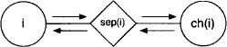
The HUGIN architecture (Jensen et al., 1990) is a modification of Lauritzen-Spiegelhalter to make the divisions less costly. It postpones division to the distribute phase such that the collect phase again corresponds to the collect algorithm with the only difference that every message is stored in the separator between the neighboring nodes i and j. These separators have the label sep(i) = λ(i) λ(j) according to Definition 3.12. They can be seen as components between join tree nodes, comparable to the mailboxes in the Shenoy-Shafer architecture. A graphical illustration is shown in Figure 4.9. Subsequently, we denote by S the set of all separators. In the following distribute phase, the messages are computed as in the Lauritzen-Spiegelhalter architecture, but have to pass through the separator lying between the sending and receiving nodes. The separator becomes activated by the crossing message and holds it back in order to divide out its current content. Finally, the modified message is delivered to the destination, and the original message is stored in the separator.

Formally, the message sent from node i to ch(i) during the collect phase is

This message is stored in the separator sep(i). In the distribute phase, node ch(i) then sends the message

towards i. This message arrives at the separator where it is altered to

(4.17)

The message is sent to node i and combined with the node content. This formula also shows the advantage of the HUGIN architecture over the Lauritzen-Spiegelhalter architecture. Divisions are performed in the separators exclusively and these have in general smaller labels than the join tree nodes. In equation (4.14) we have seen that the distribute messages in the Lauritzen-Spiegelhalter architecture correspond already to the projection of the objective function to the separator. This is also the case for the messages that are sent in the distribute phase of the HUGIN architecture and that are stored in the separators. However, the message emitted by the separator does not have this property anymore since division has been performed.

Theorem 4.3 At the end of the HUGIN architecture, each node i V stores and every separator between i and j the projection provjded that all messages during an execution of the Shenoy-Shafer architecture can be computed.

The HUGIN algorithm imposes the identical restrictions on the valuation algebra as the Lauritzen-Spiegelhalter architecture and has furthermore been identified as an improvement of the latter that makes the division operation less costly. It is therefore not surprising that the above theorem underlies the same existential condition regarding the messages of the Shenoy-Shafer architecture as Theorem 4.2. The proof of this theorem can be found in Appendix D.2.2.

Algorithm 4.5 HUGIN Architecture: Message-Passing

We again summarize this local computation scheme by a pseudo-code algorithm. Here, the factor refers to the content of the separator between node i and ch(i). However, since both theorems 4.2 and 4.3 make equal statements about the result at the end of the message-passing, we can reuse Algorithm 4.4 for the query answering in the HUGIN architecture and just redefine the message-passing procedure:

Example 4.5 We illustrate the HUGIN architecture in the same setting as Lauritzen-Spiegelhalter architecture in Example 4.4. However, since the collect phase of the HUGIN architecture is identical to the generalized collect algorithm, we directly take the messages from Examples 3.20 and 3.22. The node contents after the collect phase corresponds to Example 4.4 but without the inverses of the messages. Instead, all messages sent during the collect phase are assumed to be stored in the separators. In the distribute phase, messages are sent from the root node down to the leaves. When a message traverses a separator that stores the upward message from the collect phase, the latter is divided out of the traversing message and the result is forwarded to the receiving node. Let us consider these forwarded messages in detail:

• Node 6 obtains the message
  
  Note that the division was performed while traversing the separator node. Then, node 6 updates its content to
  
  The second equality follows from the combination axiom. For the remaining nodes, we only give the messages that are obtained in the distribute phase.
• Node 5 obtains the message
  
• Node 4 obtains the message
  
• Node 3 obtains the message
  
• Node 2 obtains the message
  
• Node 1 obtains the message
  

These messages consist of the messages from Example 4.4 from which the collect message is divided out. We therefore see that the division only takes place on the separator size and not on the node label itself.

4.4.1 Complexity of the HUGIN Architecture

Division is more efficient in the HUGIN architecture since it takes place on the separators which are generally smaller than the node labels. On the other hand, we additionally have to keep the inward messages in the memory that is not necessary in the Lauritzen-Spiegelhalter architecture. Both changes do not affect the overall complexity such that HUGIN is subject to the same time and space complexity bounds as derived for the Lauritzen-Spiegelhalter architecture in Section 4.3.1. From this point of view, the HUGIN architecture is generally preferred over Lauritzen-Spiegelhalter. An analysis for the time-space trade-off between the HUGIN and Shenoy-Shafer architecture based on Bayesian networks has been drawn by (Allen & Darwiche, 2003), and we again refer to (Lepar & Shenoy, 1998) where all three multi-query architectures are juxtaposed. We are now going to discuss one last local computation scheme for the solution of multi-query inference problems that applies to idempotent valuation algebras. In some sense, and this already foreshadows its proof, this scheme is identical to the Lauritzen-Spiegelhalter architecture where division is simply ignored because it has no effect in an idempotent valuation algebra.

4.5 THE IDEMPOTENT ARCHITECTURE

Section 4.2.1 introduces idempotency as a strong algebraic property under which division becomes trivial. Thus, the Lauritzen-Spiegelhalter as well as the HUGIN architecture can both be applied to inference problems with factors from an idem-potent valuation algebra. Clearly, if division in these architectures does not provoke any effect, we can ignore its execution altogether. This leads to the most simple local computation scheme called idempotent architecture (Kohlas, 2003).

In the Lauritzen-Spiegelhalter architecture, the message sent from i to ch(i) during the collect phase is divided out of the node content. Since idempotent valuations are their own inverses, this reduces to a simple combination. Hence, instead of dividing out the emitted message, it is simply combined to the content of the sending node. By idempotency, this combination has no effect. Thus, consider the collect message

This message is divided out of the node of i:

The last equality follows from idempotency. Consequently, the idempotent architecture consists in the execution of the collect algorithm towards a previously fixed root node m followed by a simple distribute phase where incoming messages are combined to the node content without any further action. In particular, no division needs to be performed. This derives the idempotent architecture from Lauritzen-Spiegelhalter, but it also follows in a similar way from the HUGIN architecture (Pouly, 2008). To sum it up, the architectures of Lauritzen-Spiegelhalter and HUGIN both simplify to the same scheme where no division needs to be done.

Theorem 4.4 At the end of the idempotent architecture, node i contains .

This theorem follows from the correctness of the Lauritzen-Spiegelhalter architecture and the above considerations. Further, there is no need to condition the statement on the existence of the Shenoy-Shafer messages since idempotent valuation algebras are always regular. This is shown in Appendix D.1.3. For the pseudo-code algorithm, we may again restrict ourselves to the message-passing part and refer to Algorithm 4.4 for the query answering procedure.

Algorithm 4.6 Idempotent Architecture: Message-Passing

Example 4.6 If we again call in the same setting as for the Lauritzen-Spiegelhalter and HUGIN architecture in Example 4.4 and 4.5 for the illustration of the idempotent architecture, things become particularly simple (as it is often the case with the idem-potent architecture). The collect phase executed the generalized collect algorithm whose messages can be found in Example 3.20 and 3.22. Then, the distribute phase just continues in exactly the same way:

• Node 6 obtains the message
  
  and updates its node content to
  
  The second equality follows from the combination axiom. Since corresponds to a projection of 6 it follows from idempotency that
  
  This explains the third equality. For the remaining nodes, we only give the messages that are obtained in the distribute phase.
• Node 5 obtains the message
  
• Node 4 obtains the message
  
• Node 3 obtains the message
  
• Node 2 obtains the message
  
• Node 1 obtains the message
  

Observe that no division has been performed anywhere.

4.5.1 Complexity of the Idempotent Architecture

The idempotent architecture is absolutely symmetric concerning the number of executed operations. There are 2(|V| - 1) exchanged messages, thus 2(|V| - 1) projections and 2(|V| - 1) combinations to perform. No division is performed anywhere in this architecture. Further, each message can directly be discarded once it has been combined to the node content of its receiver. Thus, although we obtain the same bounds for the time and space complexity as in the Lauritzen-Spiegelhalter and HUGIN architecture, the idempotent architecture can be considered as getting the best of both worlds. Since no division is performed, the idempotent architecture even outperforms the HUGIN scheme and does not need to remember any messages. Thus, if time is the more sensitive resource and idempotency holds, the idempotent architecture becomes the best choice to solve multi-query inference problems by local computation. Moreover, if we are dealing with a valuation algebra where both complexities are polynomial, the idempotent architecture provides a specialized query answering procedure for queries that are not covered by the join tree. This procedure is presented in the following section.

4.6 ANSWERING UNCOVERED QUERIES

The concept of a covering join tree ensures that all queries from the original inference problem can be answered after the completed distributed phase. But if later a new query arrives that is not covered by any of the join tree nodes, it is generally necessary to construct a new join tree and to execute the local computation architecture from scratch. Alternatively, there are updating methods described in (Schneuwly, 2007) that modify the join tree to cover the new query. Then, only a part of the complete message-passing has to be re-processed. However, a third option that is especially suited for formalisms with a polynomial complexity exists in the idempotent case. This method is a consequence of an interesting property of the idempotent architecture that is concerned with a particular factorization of the objective function. Initially, the original factorization of the objective function is given in the definition of the inference problem. Then, a second factorization is obtained from Lemma 3.8 with the property that the domain of each factor is covered by some specific node of the join tree. In case of idempotency, we obtain a third factorization of the objective function from the node contents after local computation:

Lemma 4.4 In an idempotent valuation algebra we have

(4.18)

Proof: The proof of this lemma is based on the correctness of the Lauritzen-Spiegelhalter architecture, which can always be executed when idempotency holds. At the beginning, we clearly have

During the collect phase, each node computes the message for its child node and divides it out of its node content. Then, the message is sent to the child node where it is combined to the node content. Thus, each message that is divided out of some node content is later combined to the content of another node. We therefore conclude that the above equation still holds at the end of the collect phase in the Lauritzen-Spiegelhalter architecture. Formally, equation (4.13) defines the node content at the end of the collect phase in the Lauritzen-Spiegelhalter architecture and we thus have

By idempotency it further holds that

and therefore

But the marginal of with respect to λ(i) λ(ch(i)) corresponds exactly to the message sent from node ch(i) to node i during the distribute phase of the Lauritzen-Spiegelhalter architecture, see equation (4.14). We therefore have by the correctness of the Lauritzen-Spiegelhalter architecture

As a consequence of this result, we may consider local computation as a transformation of the join tree factorization of Lemma 3.8 into a new factorization where each factor corresponds to the projection of the objective function to some node label. The following theorem provides a further generalization of this statement.

Theorem 4.5 For i = 1, …, r and

(4.19)

it holds for an idempotent valuation algebra that

(4.20)

Proof: We proceed by induction: For i = 1 the statement follows from Lemma 4.4 and from the domain axiom. For i + 1 we observe that and obtain using the induction hypothesis and the combination axiom

From the running intersection property we further derive λ(i)λ(ch(i)) = λ(i)yi+1 and obtain by idempotency

We next observe that combining the node content of two neighboring nodes always results in the objective function projected to their common domain.

Lemma 4.5 For 1 ≤ i, j ≤ r and j ne(i) we have

Proof: We remark that if i and j are neighbors, then either i = ch(j) or j = ch(i). It is therefore sufficient to prove the following statement:

(4.21)

It follows from Theorem 4.5, idempotency and the combination axiom that

We further conclude from equation (4.19) that

and finally obtain

This lemma states that if a new query x d() arrives that is not covered by the join tree, it can nevertheless be answered if we find two neighboring nodes whose union label covers the query, i.e. . We then compute

Thus, we neither need a new join tree nor a new propagation to answer this query. However, it is admittedly a rare case that two neighboring nodes can be found that cover some new query. The following lemma therefore generalizes this procedure to paths connecting two arbitrary nodes in the join tree.

Lemma 4.6 Let (p1, …, pk) be a path from node p1 to node pk with pi V for 1 ≤ i ≤ k. We then have for an idempotent valuation algebra

(4.22)

Proof: We proceed by induction over the length of the path: For i = 2 we have p1 ne(p2) and the statement follows from Lemma 4.5. For a path (p1, …, pk+1) we merge the nodes {p1, …, pk} to a single node called z to which all neighbors of p1 to pk are connected. The label of node z is . Clearly, the running intersection property is still satisfied in the new tree. Since pk+1 ne(z) we may again apply Lemma 4.5 and obtain,

The last equality follows from the induction hypothesis.

It then follows immediately from this lemma and the transitivity of projection that

(4.23)

This allows us to express the following yet rather inefficient procedure to answer a query x d() that is covered by the union label of two arbitrary join tree nodes:

We here assume for simplicity that the query is split over only two nodes. If more than two nodes are necessary to cover the query, it is easily possible to generalize Lemma 4.6 to arbitrary subtrees of the join tree instead of only paths. Clearly, this simple procedure is very inefficient and almost amounts to a naive computation of the objective function itself, due to the combination of all node factors on the path between i and j in the second step. However, there is a more intelligent way to perform these computations that only requires combining the content of two neighboring nodes. This is the statement of the following lemma:

Lemma 4.7 In an idempotent valuation algebra, it holds that

Proof: It follows from the transitivity axiom, Lemma 4.6, the combination axiom and the running intersection property that

We now give an algorithm similar to the above procedure that exploits Lemma 4.7 to avoid the combination of all node factors on the path between node p1 and pk.

Algorithm 4.7 Specialized Query Answering

Theorem 4.6 Algorithm 4.7 outputs .

Proof: Let us first show that the projection of in the loop is well-defined. After repetition i of the loop we have:

(4.24)

In loop is projected to . Hence, this projection is feasible. We next prove that

(4.25)

holds at the end of the loop. The statement of the theorem then follows by the transitivity of projection. For k = 2 it follows from Lemma 4.6 that

The second equality follows by initialization and the third from the domain axiom. This proves the correctness of the algorithm for paths of length 2. We now assume that equation (4.25) holds for paths of length k. For a path of length k + 1, the last repetition of the loop computes

The first equality follows from the induction hypothesis, the second from transitivity and the third from lemma 4.7. This proves the correctness of equation (4.25 and the statement of the theorem follows by the transitivity of projection.

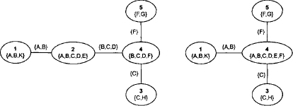
Example 4.7 We want to answer the new query × = {A, B} in the join tree of Figure 4.3 after a complete run of the idempotent architecture. We immediately see that this query is not covered by the join tree, but it is for example covered by the union label of the two nodes 1 and 6, i.e. x . The path between these two nodes has already been shown in Figure 4.10. The following three steps are executed by Algorithm 4.7:

Finally, the algorithm returns

A closer look on Algorithm 4.7 or more precisely on equation (4.24) shows that we may extract a lot more information from the intermediate results

for 1 ≤ i ≤ k. In fact, it is not only possible to compute the final query as stated in Theorem 4.6, but we actually obtain all possible queries that are subsets of λ(p1) ∪ λ(pi) by just one additional projection per query. This is the statement of the following complement to Theorem 4.6.

Lemma 4.8 Let (p1, …, pk) be a path from node p1 to node pk. Algorithm 4.7 can be adapted to compute for all x λ(p1) ∪ λ(pi) for i = 2, …, k.

Example 4.8 From the intermediate results of Example 4.7 we may compute all possible queries that are subsets of {A, T, E, L, T} and {A, T, B, E, L} by just one additional projection per query. This includes in particular the binary queries {A, E}, {A, L} and {T, B} which are not covered by the join tree in Figure 4.3.

A further extension of Algorithm 4.7 provides for a previously fixed node a pre-compilation of the join tree such that all possible queries, that are subsets of λ(i) ∪ λ(j) for all nodes j V, can be computed by just one additional projection per query. To do so, we start with the selected node i and compute for each neighbor k ne(i) the projection of to λ(i) ∪ λ(k). This intermediate result is stored in the neighbor node k. Then, the process continues for all neighbors of node k that have not yet been considered. If l ne(k) is such a neighbor of k, we compute the projection to λ(i) ∪ λ(l) by reusing the intermediate result stored in k. This is possible due to Lemma 4.7:

At the end of this process, each node j V contains which allows us to answer all queries that are subsets of λ(i) ∪ λ(j) by just one additional projection. These projections setup another factorization of the objective function as a consequence of Lemma 4.6.

Algorithm 4.8 Compilation for Specialized Query Answering

4.6.1 The Complexity of Answering Uncovered Queries

We first point out that finding the path between two nodes in a directed tree is particularly easy. We simply compute the intersection of the two paths that connect both nodes with the root node. Due to equation (4.24) the loop statement of Algorithm 4.7 computes a factor of domain . Its number of repetitions is bounded by the longest possible path in the join tree, which has at most |V| nodes. We therefore conclude that Algorithm 4.7 adopts a time complexity of

(4.26)

Since only one combination of two node contents is kept in memory at every time, we obtain for the space complexity

(4.27)

Algorithm 4.8 combines the node content of each node with the content of one of its neighbors. This clearly results in the same time complexity. But in contrast, we store one such factor in each node, which gives us a space complexity of

(4.28)

for Algorithm 4.8. At first glance, the complexities of these algorithms seem very bad because they are controlled by the double of the treewidth. Especially for formalism with exponential time or space behaviour, it could therefore be more efficient to construct a new join tree that also covers the new queries and execute the complete local computation process from scratch. But whenever we add new queries to the inference problem, we risk obtaining a join tree with a larger treewidth. This makes it difficult to directly compare the two approaches. The definition of a covering join tree ensures that every query is covered by the label of a join tree node. Here, we only require that every query is covered by the union of two arbitrary node labels. We will see in Chapter 9 that important applications exist where this is always satisfied. Imagine for example that our query set consists of all possible queries of two variables {X, Y} with and X ≠ Y. Building a covering join tree for such an inference problem always leads a join tree whose largest node label contains all variables. We then compute the objective function directly and the effect of local computation disappears. On the other hand, it is always guaranteed that such queries are covered by the union label of two join tree nodes. We can therefore ignore the query set in the join tree construction process and obtain the best possible join tree that can be found for the current knowledgebase. Later, queries are answered by the above procedures which clearly is more efficient than computing the objective function directly. Chapter 9 shows that such particular query sets frequently occur when local computation is used for the solution of path problems in sparse networks. Then, the query {X, Y} for example represents the shortest distance between two network hosts X and Y, and the query set of all possible pairs of variables models the so-called all-pairs shortest path problem.

We have now seen several important concepts that are all related to a division operator in the valuation algebra: namely, two local computation architectures that directly exploit division and the particularly simple idempotent architecture, including a specialized procedure to answer uncovered queries. In addition, the presence of inverse elements allows us to introduce the notion of scaling or normalization on an algebraic level and also to derive variations of local computation architectures that directly compute scaled results. This is the subject of the next section.

4.7 SCALING AND NORMALIZATION

Scaling or normalization is an important notion in a couple of valuation algebra instances. If, for example, we want to use arithmetic potentials to represent discrete probability distributions, it is semantically important that all values sum up to one. Only in this case are we allowed to talk about probabilities. Similarly, normalized set potentials from Instance 1.4 adopt the semantics of belief functions (Shafer, 1976). As mentioned above, the algebraic background for the introduction of a generic scaling operator is a separative valuation algebra. It is shown in this section how scaling can be introduced potentially in every valuation algebra that fulfills this mathematical property. Nevertheless, we emphasize that there must also be a semantical reason that demands a scaling operator, and this cannot be treated on a purely algebraic level.

Following (Kohlas, 2003), we define the scaling or normalization of by

(4.29)

It is important to note that because separativity is assumed, scaled valuations do not necessarily belong to Φ but only to the separative embedding Φ*. For simplicity and because this holds for all instances presented in this book, we subsequently assume that for all . This ensures that all projections of to t to t are defined, although we are dealing with a valuation algebra with partial projection. We refer to (Kohlas, 2003) for a more general study of scaling without this additional assumption. However, to gain further insights into scalable valuation algebras, we require some results derived for separative valuation algebras in Appendix D.1.1. This is necessary to obtain the following equation and for the proof of Lemma 4.9. Nevertheless, it is possible to understand these statements without knowledge of separative valuation algebras.

Combining both sides of equation (4.29) with leads to

(4.30)

according to the theory of separative valuation algebras. A valuation and its scale are contained in the same group. The following lemma lists some further elementary properties of scaling. It is important to note that these properties only apply if the scale of a valuation is again contained in the original algebra Φ. This is required since scaling is only defined for elements in Φ.

Lemma 4.9

(4.33)

The first property of Lemma 4.9 states that scaling an already scaled valuation has no effect. Second, the combination of scaled valuations does not generally lead to a scaled valuation anymore. But computing a scaled combination does not require scaling the factors of the combination. Finally, the third statement states that projection and scaling are interchangeable. The proof can be found an Appendix D.3

In a separative valuation algebra with null elements, every null element zs forms itself a group that is a consequence of cancellativity. Therefore, null elements are inverse to themselves and consequently

(4.34)

If the separative valuation algebra has neutral elements according to Section 3.3, their scale is generally not a neutral element anymore. This property however is guaranteed if the valuation algebra is stable. It follows from (4.30) that

(4.35)

Let be the set of all scaled valuations, i.e.

(4.36)

The operation of labeling is well-defined in . If we assume furthermore that all scales are element of Φ, i.e. , we know from Lemma 4.9 that is also closed under projection. However, since a combination of scaled valuations does generally not yield a scaled valuation anymore, we define

(4.37)

Note that Lemma 4.9 also implies

(4.38)

The requirement that all scales are elements of Φ holds in particular if the valuation algebra is regular. If even idempotency holds, every valuation is the scale of itself,

(4.39)

Consequently, we have in case of idempotency.

Theorem 4.7 Assume . Then, , D with the operations of labeling d, combination , and projection is a valuation algebra.

Proof: We verify the axioms from Section 1.1 on , D:

(A1) Commutative Semigroup: Commutativity of follows directly from (4.37). Associativity is derived as follows:

(A2) Labeling: Since a valuation and its scale both have the same domain,

(A3) Projection: For with d() = x we have

(A4) Transitivity: For it follows that

(A5) Combination: For with and such that we have

(A6) Domain: For and d() = x,

Accepting the requirement that , the mapping is a homomorphism from to , D. The latter is called scaled valuation algebra associated with . Finally, in a valuation algebra with adjoined identity element e, this element is not affected from scaling. From e = e−1 follows that

(4.40)

Let us now consider two examples of separative valuation algebras with a semantical requirement for scaling. A third example can be found in Appendix D.3 of this chapter and in Appendix E.5 of Chapter 5.

4.4 Probability Potentials

Normalized arithmetic potentials often take a preferred position because they adopt the interpretation of discrete probability distributions. An arithmetic potential p with domain s is normalized if its values sum up to one, i.e. if

This is achieved by applying the generic scaling operation of Definition 4.29:

(4.41)

We illustrate this process by applying the scaling operation to the arithmetic potential p3 from Instance 1.3. Since we obtain

4.5 Probability Density Functions

Continuous probability distributions are a particularly important class of density functions and motivate our interest in normalized densities. According to equation (4.29), the scale of a density function with d(f) = s is

(4.42)

for . Consequently, we have for a scaled density

Obtaining scaled results from the computation of an inference problem is an essential requirement for many applications. We may deduce from the second property of Lemma 4.9 that the result of computing a query of an inference problem will not necessarily lead to a scaled valuation again, even though the knowledgebase of the inference problem consists of only scaled valuations. This problem will be analyzed in the following section. To do so, we should also be aware of the computational effort of executing a scaling operation on some valuation . We know from equation (4.29) that the scale of is obtained by combining with the inverse of its projection to the empty domain. Scaling therefore requires executing one projection and one combination. The inverse is computed on the empty domain for all valuations and can therefore be neglected, i.e. this effort is constant for all valuations.

4.8 LOCAL COMPUTATION WITH SCALING

Let us now focus on the task of computing scaled queries from a knowledgebase where and . We derive from Lemma 4.9 that

This derivation provides different possibilities. The first expression is the straightforward approach: we compute each query using some local computation architecture and perform a scaling operation on the result. This requires |x| scaling operations, thus |x| combinations but only one projection since the inverse of the objective function projected to the empty domain is identical for all queries. The second expression performs only a single scaling operation on the total objective function. However, we directly refuse this approach since it requires explicitly building the objective function . A third approach follows from the last expression if we additionally suppose that all scales are contained in Φ, i.e. that . We then know from Theorem 4.7 that we may directly compute in the valuation algebra . However, this is again worse than the straightforward approach since it executes one scaling operation per combination during the local computation process as a result of equation (4.38).

A far more promising approach arises if we integrate scaling directly into the local computation architectures. Since the underlying valuation algebra is assumed to be separative, we can potentially use the Shenoy-Shafer, Lauritzen-Spiegelhalter or HUGIN architecture. Furthermore, if the valuation algebra is idempotent, we do not need to care about scaling at all because idempotent valuations are always scaled. Thus, we are next going to reconsider the three architectures above and show that only a single execution of scaling in the root node of the join tree is sufficient in each of them to scale all query answers. This is well-known in the context of Bayesian networks, and for general valuation algebras it was shown by (Kohlas, 2003).

4.8.1 The Scaled Shenoy-Shafer Architecture

The scaled Shenoy-Shafer architecture first executes the collect phase so that the projection of the objective function to the root node label λ(r) can be computed in the root node . Then, the root content r is replaced by

(4.43)

When the distribute phase starts, the outgoing messages from the root node are computed from this modified node content. The result of this process is stated in the following theorem.

Theorem 4.8 At the end of the message-passing in the scaled Shenoy-Shafer architecture, we obtain at node i

(4.44)

where are the modified messages from the scaled architecture.

Proof: The messages of the collect phase do not change, i.e. . For the distribute messages, we show that

(4.45)

The distribute message sent by the root node to parent i is

This follows from the combination axiom. Hence, equation (4.45) holds for all messages that are emitted by the root node. We proceed by induction and assume that the proposition holds for . Then, by application of the combination axiom, we have for all

By Theorem 4.1 we finally conclude that

To sum it up, the execution of one single scaling operation in the root node scales all projections of the objective function in the Shenoy-Shafer architecture. We summarize this modified Shenoy-Shafer architecture in terms of a pseudo-code algorithm. Since the modification only concerns the message-passing, only Algorithm 4.1 must be adapted.

Algorithm 4.9 Scaled Shenoy-Shafer Architecture: Message-Passing

4.8.2 The Scaled Lauritzen-Spiegelhalter Architecture

The Lauritzen-Spiegelhalter architecture first executes the collect algorithm with the extension that emitted messages are divided out of the node content. At the end of this collect phase, the root node directly contains the projection of the objective function to the root node label λ(r). We pursue a similar strategy as in the scaled Shenoy-Shafer architecture and replace the root content by its scale

(4.46)

Then, the distribute phase proceeds as usually.

Theorem 4.9 At the end of the scaled Lauritzen-Spiegelhalter architecture, node i contains provided that all messages during an execution of the

Shenoy-Shafer architecture can be computed.

Proof: By equation (4.46), the theorem is satisfied for the root node. We proceed by induction and assume that the proposition holds for the node ch(i) which therefore contains . The content of node i in turn is given by equation (4.13). Applying Theorem 4.2 gives

Again, a single execution of scaling in the root node scales all results in the Lauritzen-Spiegelhalter architecture. We again give the required modification of Algorithm 4.3 explicitly:

Algorithm 4.10 Scaled Lauritzen-Spiegelhalter Architecture: Message-Passing

4.8.3 The Scaled HUGIN Architecture

Scaling in the HUGIN architecture is equal to Lauritzen-Spiegelhalter. We again execute the collect phase and modify the root content according to equation (4.46). Then, the outward phase starts in the usual way.

Theorem 4.10 At the end of the computations in the HUGIN architecture, each node i V stores and every separator between i and j the projection provided that all messages during an execution of the Shenoy-Shafer architecture can be computed.

Proof: By equation (4.46), the theorem is satisfied for the root node. We proceed by induction and assume that the proposition holds for node ch(i). Then, the separator lying between i and ch(i) will update its stored content to

Node i contains ′i when receiving the forwarded separator content and computes

Once more, a single execution of scaling in the root node scales all results in the HUGIN architecture. It follows the corresponding adaption of Algorithm 4.5.

Algorithm 4.11 Scaled HUGIN Architecture: Message-Passing

These adaptions for scaling close the discussion of local computation. Further local computation schemes but for an extended computational task will be introduced in Chapters 9 and 8.

4.9 CONCLUSION

The topic of this chapter was the solution of inference problems where multiple queries have to be computed. We quickly remarked that a repeated application of the generalized collect algorithm for each query leads to a lot of redundant computations. On the other hand, a more detailed analysis has shown that two such runs differ only in the messages sent between the two root nodes. This fact is exploited by the Shenoy-Shafer architecture that solves a multi-query inference problem by only the double number of messages used for the computation of a single query. In addition, since the Shenoy-Shafer architecture stores messages in mailboxes instead of combining them to the node content, we obtain the best possible space complexity one can expect for a general local computation scheme. However, the prize we have to pay is that a lot of redundant operations are still performed, unless particular join trees such as binary join trees are used. This was the key motivation for the introduction of further local computation procedure with a more sophisticated caching policy. These architectures benefit from a division operation that is in general not present in a valuation algebra. We therefore discussed three different, algebraic properties in the appendix of this chapter that allow the introduction of division: if the valuation algebra is separative, it can be embedded into a union of groups which naturally provide inverse elements. This is the most general property and leads to an extension of the original valuation algebra where division is possible but where projection is only partially defined. Alternatively, if the valuation algebra is regular, it decomposes directly into a union of groups and full projection is conserved. The third and strongest property is idempotency. In this case, every element is the inverse of itself and division becomes trivial. Back to local computation, we developed two specialized architectures that apply to separative (and hence regular) valuation algebras. The Lauritzen-Spiegelhalter architecture executes the collect algorithm in its inward phase but always divides the message for the child node out of each node content. This ensures that no information is combined a second time when the distribute message arrives. Here, the division takes place on the node content and all messages can be discarded as soon as they have been combined to some node content. On the other hand, we need to store one factor per node whose size is bounded by the node label. Thus, we avoid the redundant computations of the Shenoy-Shafer architecture to the expense of a considerably higher space requirement. The second scheme called HUGIN architecture delays division to the distribute phase where it only takes place on the separators. This makes division less costly but requires to store the collect messages until the end of the message-passing. A fourth and last local computation scheme called idempotent architecture can be applied if idempotency holds in the valuation algebra. Essentially, it is equal to the Lauritzen-Spiegelhalter architecture but passes on the execution of trivial division. Thus, no additional effort is spent in division and no messages must be cached. The very strong property of idempotency further enables a specialized procedure to answer queries which are not covered by the join tree. This procedure becomes especially worthwhile when a large number of queries has to be computed. Finally, we pointed out that scaling or normalization is an important issue for many applications. From the algebraic point of view, we propose a generic definition of scaling when division is present, i.e. if the valuation algebra is at least separative. However, there must also be a semantical motivation for a scaling operation in a valuation algebra which cannot be justified on a purely algebraic level. If this requirement exists, we are naturally interested in computing scaled queries and it turned out that a slight modification of local computation architectures allows computing an arbitrary number of scaled queries with only one single execution of the scaling operation in the root node of the join tree. Figure 4.11 summarizes the local computation procedures and their algebraic requirements.

Appendix: Valuation Algebras with Division

In the first part of the appendix, we will study under which conditions valuation algebras provide a division operation. It has already been mentioned that the pure existence of inverse elements according to Definition 4.1 is not sufficient since this only refers to combination. But in order to apply division in local computation architectures, we also need a property for the projection operation. However, the definition of inverse elements is nevertheless a good starting point for the understanding of division in the context of valuation algebras, and it turns out that all properties studied below imply their existence. (Kohlas, 2003) distinguishes three different cases: Separativity is the weakest requirement. It allows the valuation algebra to be embedded into a union of groups that naturally include inverse elements. However, the price we pay is that full projection gets lost and we therefore recommend reading Appendix A.3 before entering the study of separative valuation algebras. Alternatively, regularity is a stronger condition. In this case, the valuation algebra itself is decomposed into groups, such that full projection is conserved. Finally, if the third and strongest requirement called idempotency holds, every valuation turns out to be the inverse of itself. This has already been shown in Section 4.2.1 but here we are going to treat idempotency as a special case of regularity and thus separativity.

D.1 PROPERTIES FOR THE INTRODUCTION OF DIVISION

Equivalence relations play an important role in all three cases since they will be used for the decomposition of Φ. An equivalence relation γ is areflexive, symmetric and transitive relation. Thus, we have for

Since we want to partition a valuation algebra, equivalence relations that are compatible with the operations in Φ are of particular importance. Such relations are called congruences and satisfy the following properties:

An intuitive motivation for the introduction of congruences in valuation algebras is that different valuations sometimes represent the same knowledge. Thus, they are pooled in equivalence classes that are induced by such a congruence relation γ.

D.1.1 Separative Valuation Algebras

The mathematical notion of a group involves a set with a binary operation that is associative, has a unique identity and each element has an inverse. Thus, we may obtain inverse elements in a valuation algebra if the latter can be embedded into a union of groups. It is known from semigroup theory (Clifford & Preston, 1967) that the property of cancellativity is sufficient to embed a semigroup into a union of groups, and it is therefore reasonable to apply this technique also for valuation algebras which, according to Axiom (A1), form a semigroup under combination (Lauritzen & Jensen, 1997). See also Exercise A.4 in Chapter 1. However, (Kohlas, 2003) remarked that a more restrictive requirement is needed for valuation algebras that also accounts for the operation of projection. These prerequisites are given in the following definition of separativity where we assume a congruence γ that divides Φ into disjoint equivalence classes []γ given by

(D.1)

Definition D.4 A valuation algebra is called separative, if there is a congruence γ such that

• for all with we have ,
• for all and t d();

(D.2)

From the properties of a congruence, it follows that all elements of an equivalence class have the same domain. Further, the equivalence classes are closed under combination. For and thus , we conclude from (D.2)

Additionally, since all []γ are subsets of Φ, combination within an equivalence class is both associative and commutative. Hence, Φ decomposes into a family of disjoint, commutative semigroups

Semigroups obeying the first property in the definition of separativity are called cancellative (Clifford & Preston, 1967) and it follows from semigroup theory that every cancellative and commutative semigroup []γ can be embedded into a group. These groups are denoted by γ() and contain pairs (, ) of elements from []γ (Croisot, 1953; Tamura & Kimura, 1954). This is similar to the introduction of positive, rational numbers as pairs (numerator and denominator) of natural numbers. Two group elements (, ) and (′, ′) are identified if . Further, combination within γ() is defined by

(D.3)

Let Φ* be the union of those groups γ(), i.e.

We define the combination of elements by

(D.4)

It can easily be shown that this combination is well-defined, associative and commutative (Kohlas, 2003). Φ* is therefore a semigroup under . Moreover, the mapping from Φ to Φ* defined by

is a semigroup homomorphism which is furthermore one-to-one due to the cancellativity of the semigroup []γ. In this way, Φ is embedded as a semigroup into Φ*. Subsequently, we identify with its counterpart in Φ*. Since γ() are groups, they contain both inverses and an identity element. We therefore write

for the inverse of group element , and denote the identity element within γ() as fγ(). Note that neither inverses nor identity elements necessarily belong to Φ but only to Φ*. The embedding of Φ into a union of groups Φ* via its decomposition into commutative semigroups is illustrated in Figure D. 1.

We next introduce a relation between the semigroups []γ. Since γ is a congruence, we may define the combination between congruence classes as

(D.5)

and say that

(D.6)

This relation is a partial order, i.e. reflexive, transitive and antisymmetric according to Definition A.2, as shown in (Kohlas, 2003). It can further be carried over to γ() by defining

The following properties are proved in (Kohlas, 2003):

Lemma D.10

It is now possible to extend (partially) the operations of labeling, projection and combination from

• Labeling d* for elements in is defined for by for some , if . Since γ is a congruence, d* does not depend on the representative of the group . Therefore, d* is well-defined. Further, the label for an element is . In other words, d* is an extension of d, and since and are contained in the same group, we directly get .
• We have already seen in equation (D.4) how the combination is carried out among elements in . This operator also extends , since

for elements , which are identified by and respectively. With this extension of combination, we further remark that and are indeed inverses according to Definition 4.1, since

(D.7)

and

(D.8)

We therefore conclude that separativity is a sufficient property to guarantee the existence of inverse elements.

• Finally, we partially extend the operator of projection. Given an element , the projection of to a domain s is defined by

(D.9)

if there are with and such that

This definition will be justified using the following lemma.

Lemma D.11 Let, be the pair representation of an element with and d. Then can be written as

Proof: Because γ is a congruence, we have and further

Note again the similarity to positive, rational numbers represented as pairs of naturals. So, any element can at least be projected to its own domain. It will next be shown that is well-defined. Take two representations of the same element with and such that . Assume that both can be projected to a domain s, i.e. there are and such that and . We show that

(D.10)

First, we conclude from that

We multiply both sides with and obtain

thus

Since and , Lemma D.10 implies

and because extends the combination in must hold. By application of the combination axiom in

(D.11)

Next, it will be shown that

(D.12)

Since , equation (D.6) implies that and therefore

(D.13)

On the other hand, the combination axiom in yields

Therefore and using equation (D.13) we obtain . This proves the first relation of (D.12) and the second is obtained by symmetry. Finally, we deduce from multiplying both sides of (D.11) with

hence

and due to (D.12) and Lemma D.10 we finally obtain

This proves that projection in is well-defined.

It remains to be verified that is really an extension of . Let . In the first step we have to guarantee that is defined for all s . The valuation can be written as

since

and . According to Lemma D.10 we have and . Therefore, the projection of to any domain is defined. Now, using the combination axiom in ,

Note that the extended domain operator is directly induced by the definition of the new projection operator, i.e. for

(D.14)

Theorem D.11 with the operations of labeling d*, combination , domain M* and projection is a valuation algebra with partial projection.

Proof: We verify the axioms on given in Appendix A.3:

This shows that the property of separativity is sufficient to provide a valuation algebra with a division operation. Again, we point out that we loose the property of full projection by this construction. Therefore, we end with a valuation algebra with partial projection as stated by the above theorem. Before listing some instances of separative valuation algebras, we remark that cases exist where we do not need to worry about the existence of the projections in the combination axiom.

Lemma D.12 Let and and . For every domain such that s t we have z .

Proof: Since can be projected to any domain contained in , especially to , it follows from the combination axiom that z .

It is shown in (Pouly, 2008) that an identity element e can also be adjoined to a separative valuation algebra without affecting separativity. It always holds that e = e−1 that allows us to derive division-based local computation architectures from the Shenoy-Shafer architecture of Section 4.1 that uses this particular element.

D.6 Set Potentials and Separativity

In order to prove that set potentials are separative, we first introduce some alternative representations. We define for a set potential m with domain d(m) = s and A

(D.15)

Clearly, both functions bm and qm are themselves set potentials. It is furthermore shown in (Shafer, 1976) that the two transformation rules are one-to-one with the following inverse transformations

(D.16)

and

(D.17)

Consequently, the operations of combination and projection can be carried over from m-functions to b-functions and q-functions:

To sum it up, m-functions, b-functions and q-functions describe the same system, and since m-functions build a valuation algebra, the same holds for the two other representations. Additionally, we also deduce that all properties that hold for one of these representations naturally hold for the two others.

It turns out that the operations of combination and projection simplify considerably if they are expressed either in the system of q-functions or b-functions. More concretely, combination reduces to simple multiplication in the system of q-functions and projection does not need any computation at all in the system of b-functions. This is the statement of the following theorem which is for example proved in (Kohlas, 2003).

Theorem D.12

Now, we are able to show that set potentials are separative. For this purpose, we change into the system of q-functions. Then, a congruence γ is needed that divides into cancellative equivalence classes. Let us therefore introduce the support of a q-function q with d(q) = s by

q1 and q2 with equal domain are equivalent if they have the same support, i.e.

In particular, we have (mod γ) since

The second equality holds because m-functions are non-negative, projection of m-functions is defined by a sum, and q-functions are defined by a sum over the values of an m-function. Altogether, we have implies q(A) = 0 because the non-negative terms of a sum giving zero must themselves be zero. Hence, is divided into disjoint equivalence classes of q-functions with equal domain and support. These classes are cancellative since

implies that q1(A) = q2(A) if q, q1, q2 all have the same domain and support. This fulfills all requirements for separativity given in Definition D.4.

It should be mentioned that not every b-function or q-function transforms into a set potential m using either equation (D.16) or (D.17). This is because both transformations can create negative values which shows that is really an extension of the system of q-functions.

D.7 Density Functions and Separativity

In order to show that density functions are separative, we proceed similarly to the foregoing example and define the support of a density f by

Then, we again say that two densities f and g with equal domain are equivalent if they have the same support. We conclude f (mod γ) since

The second equality holds because densities are non-negative and therefore implies f(x) = 0 Hence, divides into disjoint equivalence classes of densities with equal domain and support. These classes are cancellative which fulfills all requirements for separativity given in Definition D.4.

D.1.2 Regular Valuation Algebras

We have just seen that a separative valuation algebra decomposes into disjoint semigroups which in turn can be embedded into groups. Thus, we obtain an extended valuation algebra where every element has an inverse. However, (Kohlas, 2003) remarked that in some cases, valuation algebras can directly be decomposed into groups instead of only semigroups. This makes life much easier since we can avoid the rather complicated embedding and, moreover, full projection is conserved. A sufficient condition for this simplification is the property of regularity stated in the following definition. Note also that it again extends the notion of regularity from semigroup theory to incorporate the operation of projection.

Definition D.5

• An element is called regular, if there exists for all t an element with , such that

(D.20)

• A valuation algebra is called regular, if all its elements are regular.

In contrast to the more general case of separativity, we are now looking for a congruence that decomposes directly into a union of groups. For this purpose, we introduce the Green relation (Green, 1951) between valuations:

(D.21)

denotes the set of valuations i.e. the principal ideal generated by . (Kohlas, 2003) proves that the Green relation is actually a congruence in a regular valuation algebra and that the corresponding equivalence classes []γ are directly groups which therefore provide inverse elements.

Lemma D.13 If is regular with , then and are inverses.

Proof: From Definition 4.1 we obtain

and

The equivalence classes []γ are clearly cancellative since they are groups and therefore contain inverse elements. Further, the Green relation clearly satisfies equation (D.2), which makes a regular valuation algebra also separative. From this point of view, regular valuation algebras are special cases of separative valuation algebras and since Φ does not need to be extended, full projection is preserved. This construction is illustrated in Figure D.2.

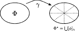
Idempotent elements play an important role in regular valuation algebras. These are elements f such that . According to Definition 4.1 we may therefore say that idempotent elements are inverse to themselves. Essentially, idempotents are obtained by combining inverses. Thus, if are inverses, is idempotent since

These idempotents behave neutral with respect to and . We have

and the same holds equally for . The following important lemma states that every principal ideal is generated by a unique idempotent valuation.

Lemma D. 14 In a regular valuation algebra there exists for all a unique idempotent f Φ with

Proof: Since is regular there is a χ such that and we know from Lemma D. 13 that and are inverses. Thus, is an idempotent such that f . Therefore, and . Consequently, must hold, and it remains to prove that f is unique. Suppose that . Then, there exists such that . This implies that . Similarly, we derive f1 and therefore it follows that f1 = f2.

We again point out that we may also adjoin an identity element to a regular valuation algebra without loosing this property. An explicit proof can be found in (Pouly, 2008). Here, we now focus on an instance of a regular valuation algebra. More examples will be given in Appendix E.2 of Chapter 5.

D.8 Arithmetic Potentials and Regularity

In Instance 4.1 we used arithmetic potentials to give a simple example of inverse elements in a valuation algebra. There, we also mentioned that arithmetic potentials are in fact regular which induces these inverse elements. Now, we are able to verify this claim. Let p be an arithmetic potential with domain s and t s. Then, the definition of regularity may be written as:

So, defining

leads naturally to a solution of this equation. Hence, the inverse of a potential p with domain s and x is given by

D.1.3 Idempotent Valuation Algebras

The property of regularity allows the decomposition of a valuation algebra into groups such that inverses exist within Φ directly. We also learned that every such group is generated from a unique idempotent element. Therefore, the last simplifying condition for the introduction of division identifies valuation algebras where every element is idempotent. This has been proposed in (Kohlas, 2003) and leads to a decomposition where every valuation forms its own group. The property of idempotency has already been defined in Definition 4.2. By choosing χ = in Definition D.5, we directly remark that every idempotent valuation algebra is regular too. Then, since principal ideals are spanned by a unique idempotent, each element of an idempotent valuation algebra generates its own principal ideal. Consequently, all groups []γ consist of the single element which is therefore also the inverse of itself.

It is not surprising that also the property of idempotency remains conserved if an identity element is adjoined to an idempotent valuation algebra. We again refer to (Pouly, 2008) for the proof of this statement. Some examples of idempotent valuation algebras have already been given in Section 4.2.1, others follow in Appendix E.4.

D.2 PROOFS OF DIVISION-BASED ARCHITECTURES

The proofs of the two division-based local computation schemes called Lauritzen-Spiegelhalter architecture and HUGIN architectures were retained in Chapter 4 since they are based on properties derived in Appendix D. 1.

D.2.1 Proof of the Lauritzen-Spiegelhalter Architecture

The proof of the Lauritzen-Spiegelhalter architecture is based on the messages used in the Shenoy-Shafer architecture. If they exist, Lauritzen-Spiegelhalter gives the correct results because the inward messages are identical in both architectures. Further, the Shenoy-Shafer messages are needed in equation (D.23) below for the application of the combination axiom. However, (Schneuwly, 2007) weakens this requirement by proving that the existence of the inward messages is in fact sufficient to make the Shenoy-Shafer architecture and therefore also Lauritzen-Spiegelhalter work.

Proof of Theorem 4.2

Proof: Let μ′ denote the messages sent during an execution of the Shenoy-Shafer architecture. We know that

during the collect propagation and the theorem holds for the root node as a result of the collect algorithm. We prove that it is correct for all nodes by induction over the outward propagation phase using the correctness of Shenoy-Shafer. For this purpose, we schedule the distribute phase by taking the reverse node numbering. When a node j is ready to send a message towards i, node i stores

(D.22)

By the induction hypothesis, the incoming message at step i is

(D.23)

The third equality follows from the combination axiom, and the assumption is needed to ensure that exists. So we obtain at node i, when the incoming message is combined with the actual content and using Theorem 4.1,

It follows from Lemma D.10 that

hence

D.2.2 Proof of the HUGIN Architecture

Proof of Theorem 4.3

Proof: The proof is based on the correctness of the Lauritzen-Spiegelhalter architecture. First we consider the separators in the join tree (V, E, λ, D) as real nodes. Thus, let (V, E′, λ′, D) be such a modified join tree. We then adapt the assignment mapping a making it again surjective. We simply assign to every separator node in V′- V the identity element e and name the extended assignment mapping a′. Now, the execution of the Lauritzen-Spiegelhalter architecture is started using (V′, E′, λ′, D, a′).

Take a node which is not a separator in the original tree. It sends a message in the collect phase of Lauritzen-Spiegelhalter and divides it out of its current content which we abbreviate with . By the construction of (V′, E′, λ′, D), the receiving node j = ch(i) is a separator in (V, E, λ, D), that is j (V′- V). Node i contains and j stores after this step. Then node j is ready to send a message towards node k = ch(j). But we clearly have . Since every emitted message is divided out of the store, the content of node j becomes

We continue with Lauritzen-Spiegelhalter and assume that node k is ready to send the message for node j during the distribute phase. This message equals due to Theorem 4.2 and also becomes the new content of j according to equation (D.23). The message sent from j towards i is finally so that we get there

This follows again from the correctness of Lauritzen-Spiegelhalter. But

is also the message from k towards i in the HUGIN architecture using (V, E, λ, D, a), which has passed already through the separator j.

The messages used throughout the proof correspond to the Lauritzen-Spiegelhalter messages. Therefore, we may conclude that the existence of the collect messages is also a sufficient condition for Theorem 4.3. If, on the other hand, the valuation algebra is regular, this condition can again be dropped.

D.3 PROOF FOR SCALING IN VALUATION ALGEBRAS

Proof of Lemma 4.9

Proof:

D.9 Scaling of Belief Functions

In Instance D.6 we derive the two alternative representations of set potentials as b-functions and q-functions. These systems are isomorphic, which allows us to conclude that they all form valuation algebras and satisfy the same additional properties. Since combination corresponds to simple multiplication in the case of q-functions, it is often convenient to study related algebraic properties in this system. Thus, we obtain by applying the definition of scaling to a q-function:

It is important to note that consists of two values, and . Since the empty set can never be obtained from projecting a non-empty configuration set, the formula can be written for the case where and as

(D.24)

We then obtain for the denominator

Since

we have for the empty set

(D.25)

So, the scale of a q-function is obtained by equation (D.24) and (D.25), and it is common to refer to non-negative, scaled q-functions as commonality functions.

We next translate the scaling operation for q-functions to the system of m-functions using equation (D.17) and obtain

(D.26)

if and . Finally, we obtain for

Thus, the scale of a set potential is given by equation (D.26) if A and , and otherwise. This satisfies the two properties:

(D.27)

In the theory of evidence, such potentials are called basic probability assignments or mass functions. Intuitively, m(A) represents the part of our belief that the actual world (i.e. some configuration) belongs to A – without supporting any more specific subset, by lack of adequate information (Smets, 2000; Smets & Kennes, 1994). Under this interpretation, the two normalization conditions imply that no belief is held in the empty configuration set (which corresponds to a closed world assumption) and that the total belief has measure 1. In a similar way, the operation of scaling can also be translated to the system of b-functions using equation (D.15). It is then common to refer to non-negative, scaled b-functions as belief functions. A comprehensive theory of mass, belief and commonality functions is contained in (Shafer, 1976). We also pointed out in Lemma 4.9 that the combination of two normalized set potentials (mass functions) does generally not lead to a mass function again. However, this can be achieved using equation (4.32). Assume two mass functions m1 and m2 with domains s and t. We have for

where

We further define m1 m2 = 0 and, if K = 0, we set m1 m2(A) = 0. This operation is called Dempster’s rule of combination (Dempster, 1968).

We complete the study of scaling for set potentials and our excursion to Dempster-Shafer theory by a small example of normalizing a set potential. Let r = {A,B} be a set of variables with finite frames and and m a set potentials with domain d(m) = {A,B} defined as:

We then compute

and obtain for its associated mass function

PROBLEM SETS AND EXERCISES

D.1 * Exercise B.4 in Chapter 2 asked to transform the fundamental computational problems of filtering, prediction and smoothing in hidden Markov chains into an inference problem. Show that the filtering and smoothing problem can simultaneously be solved by a complete run of the Shenoy-Shafer, Lauritzen-Spiegelhalter or HUGIN architecture, i.e. that filtering corresponds to the collect phase and smoothing to the distribute phase in the three local computation architectures.

D.2 * Section 4.5 derives the idempotent architecture from the correctness of the Lauritzen-Spiegelhalter architecture.

D.3 ** Consider a join tree (V, E, λ, D) with |V| = r that is fully propagated by the Shenoy-Shafer architecture, i.e. for each node we have

as stated in Theorem 4.1. Assume now that a new valuation is combined to some covering node k V with . This is called a consistent update. If the Shenoy-Shafer architecture is repeated from scratch, we obtain at the end of the message-passing for each node

where for and . However, instead of recomputing all messages , it is more appropriate to reuse the messages that do not change by this updating process. Prove that during the collect phase, only the messages between the node k and the root node change. In the distribute phase, all messages must be recomputed. Perform the same analysis for the Lauritzen-Spiegelhalter, HUGIN and idempotent architecture. The solution can be found in Chapter 6 of (Schneuwly, 2007).

D.4 * Let be an idempotent valuation algebra. For we define

(D.28)

This expresses that the information piece is more informative than .

D.5 ** Let be an information algebra and suppose that the information content of an element has been asserted. Then, all information pieces which are less informative than should also be true. The sets

(D.29)

are called principal ideals. Observe that principal ideals are closed under combination, i.e. if , v then . We further define

and introduce the following operations in :

Prove that the set of principal ideals IΦ is closed under combination and projection, and show that satisfies the axioms of an information algebra. Indications can be found in (Kohlas, 2003), Section 6.2.

D.6 ** Let s, t,u D be disjoint sets of variables and assume that we want to define a valuation with by specifying its projections and relative to and . Of course, the projections must be consistent such that holds. The problem of finding such a valuation is called marginal problem. Intuitively, this is similar to the specification of a building by its floor, body and sheer plan. Prove that if is a regular valuation algebra according to Definition D.5, then there exists with such that

The solution to this exercise can be found in (Kohlas, 2003), Theorem 5.15. Marginal problems are closely related to the notion of conditional independence in valuation algebras that is treated in Exercise D.7.

D.7 ** Let be a valuation algebra and are disjoint subsets of d(), we say that s is conditionally independent of t given u with respect to , if there exist such that and

(D.30)

If s is conditionally independent of t given u, we write .

(G1)

(G2)

If furthermore the valuation algebra has neutral elements, we have

(G3)

The solution to these exercises can be found in Section 5.1 of (Kohlas, 2003).

D.8 ** Consider the definition of conditional independence in Exercise D.7. For u = Ø we use the short notation and say that s is independent of t with respect to . Let be a regular valuation algebra, and s,t D disjoint subsets of d(). Then, the valuation

(D.31)

is called the conditional of for s given t.

The solution to these exercises can be found in Section 5.1 of (Kohlas, 2003).

D.9 ** Exercise D.8 can be generalized to separative valuation algebras, see Appendix D.1.1. The same definition of conditionals applies in this case, but in contrast, the conditionals do generally not belong to Φ but only to the separative embedding Φ*. Also, the properties listed in Exercise D.8.b still hold in the separative case, although we must pay attention to partial projection in the proofs. Identify the conditional s|t in the valuation algebras of density functions, Gaussian potentials and set potentials. The solution to this exercises can be found in Section 5.3 of (Kohlas, 2003).