

Chapter Seven
PROBABILITY
Contents
7.2 Cumulative Distribution Functions and Probability
Cumulative Distribution Function for Ages
7.1 DENSITY FUNCTIONS
Understanding the distribution of various quantities through the population can be important to decision makers. For example, the income distribution gives useful information about the economic structure of a society. In this section we look at the distribution of ages in the US. To allocate funding for education, health care, and social security, the government needs to know how many people are in each age group. We see how to represent such information by a density function.
US Age Distribution
Table 7.1 Distribution of ages in the US in 2000


Figure 7.1: How ages were distributed in the US in 2000
Suppose we have the data in Table 7.1 showing how the ages of the US population1 were distributed in 2000. To represent this information graphically we use a type of histogram2 putting a vertical bar above each age group in such a way that the area of each bar represents the percentage in that age group. The total area of all the rectangles is 100% = 1. We only consider people who are less than 100 years old.3 For the 0–20 age group, the base of the rectangle is 20, and we want the area to be 29%, so the height must be 29%/20 = 1.45%. We treat ages as though they were continuously distributed. The category 0–20, for example, contains people who are just one day short of their twentieth birthday. Notice that the vertical axis is measured in percent/year. (See Figure 7.1.)
| Example 1 | In 2000, estimate what percentage of the US population was:
(a) Between 20 and 60 years old? (b) Less than 10 years old? (c) Between 75 and 80 years old? (d) Between 80 and 85 years old? |
| Solution | (a) We add the percentages, so 29% + 26% = 55%.
(b) To find the percentage less than 10 years old, we could assume, for example, that the population was distributed evenly over the 0–20 group. (This means we are assuming that babies were born at a fairly constant rate over the last 20 years, which is probably reasonable.) If we make this assumption, then we can say that the population less than 10 years old was about half that in the 0–20 group, that is, 14.5%. Notice that we get the same result by computing the area of the rectangle from 0 to 10. (See Figure 7.2.) (c) To find the population between 75 and 80 years old, since 13% of Americans in 2000 were in the 60-80 group, we might apply the same reasoning and say that (d) Again using the (faulty) assumption that ages in each group were distributed uniformly, we would find that the percentage between 80 and 85 was
Figure 7.2: Ages in the US in 2000—various subgroups (for Example 1) |

Smoothing Out the Histogram
We could get better estimates if we had smaller age groups (each age group in Figure 7.1 is 20 years, which is quite large) or if the histogram were smoother. Suppose we have the more detailed data in Table 7.2, which leads to the new histogram in Figure 7.3.
As we get more detailed information, the upper silhouette of the histogram becomes smoother, but the area of any of the bars still represents the percentage of the population in that age group. Imagine, in the limit, replacing the upper silhouette of the histogram by a smooth curve in such a way that area under the curve above one age group is the same as the area in the corresponding rectangle. The total area under the whole curve is again 100% = 1. (See Figure 7.3.)
The Age Density Function
If t is age in years, we define p(t), the age density function, to be a function which “smooths out” the age histogram. This function has the property that

Table 7.2 Ages in the US in 2000 (more detailed)
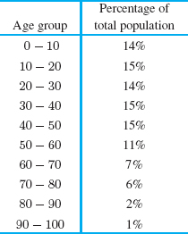

Figure 7.3: Smoothing out the age histogram
If a and b are the smallest and largest possible ages (say, a = 0 and b = 100), so that the ages of all of the population are between a and b, then
![]()
What does the age density function p tell us? Notice that we have not talked about the meaning of p(t) itself, but only of the integral ![]() Let's look at this in a bit more detail. Suppose, for example, that p(10) = 0.014 = 1.4% per year. This is not telling us that 1.4% of the population is precisely 10 years old (where 10 years old means exactly 10, not
Let's look at this in a bit more detail. Suppose, for example, that p(10) = 0.014 = 1.4% per year. This is not telling us that 1.4% of the population is precisely 10 years old (where 10 years old means exactly 10, not ![]() not
not ![]() 10.1). However, p(10) = 0.014 does tell us that for some small interval Δt around 10, the fraction of the population with ages in this interval is approximately p(10) Δt = 0.014 Δt. Notice also that the units of p(t) are % per year, so p(t) must be multiplied by years to give a percentage of the population.
10.1). However, p(10) = 0.014 does tell us that for some small interval Δt around 10, the fraction of the population with ages in this interval is approximately p(10) Δt = 0.014 Δt. Notice also that the units of p(t) are % per year, so p(t) must be multiplied by years to give a percentage of the population.
The Density Function
Suppose we are interested in how a certain numerical characteristic, x, is distributed through a population. For example, x might be height or age if the population is people, or might be wattage for a population of light bulbs. Then we define a general density function with the following properties:
The function, p(x), is a density function if

The density function must be nonnegative if its integral always gives a fraction of the population. The fraction of the population with x between −∞ and ∞ is 1 because the entire population has the characteristic x between −∞ and ∞. The function p that was used to smooth out the age histogram satisfies this definition of a density function. Notice that we do not assign a meaning to the value p(x) directly, but rather interpret p(x) Δx as the fraction of the population with the characteristic in a short interval of length Δx around x.
| Example 2 | Figure 7.4 gives the density function for the amount of time spent waiting at a doctor's office.
(a) What is the longest time anyone has to wait? (b) Approximately what fraction of patients wait between 1 and 2 hours? (c) Approximately what fraction of patients wait less than an hour?
Figure 7.4: Distribution of waiting time at a doctor's office |
| Solution | (a) The density function is zero for all t > 3, so no one waits more than 3 hours. The longest time anyone has to wait is 3 hours.
(b) The fraction of patients who wait between 1 and 2 hours is equal to the area under the density curve between t = 1 and t = 2. We can estimate this area by counting squares: There are about 7.5 squares in this region, each of area (0.5)(0.1) = 0.05. The area is approximately (7.5)(0.05) = 0.375. Thus about 37.5% of patients wait between 1 and 2 hours. (c) This fraction is equal to the area under the density function for t < 1. There are about 12 squares in this area, and each has area 0.05 as in part (b), so our estimate for the area is (12)(0.05) = 0.60. Therefore, about 60% of patients see the doctor in less than an hour. |

Problems for Section 7.1
In Problems 1–4, the distribution of the heights, x, in meters, of trees is represented by the density function p(x). In each case, calculate the fraction of trees which are:
(a) Less than 5 meters high
(b) More than 6 meters high
(c) Between 2 and 5 meters high
1.

2.

3.

4.

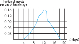
5. The density function p(t) for the length of the larval stage, in days, for a breed of insect is given in Figure 7.5. What fraction of these insects are in the larval stage for between 10 and 12 days? For less than 8 days? For more than 12 days? In which one-day interval is the length of a larval stage most likely to fall?
6. Figure 7.64 shows the distribution of elevation, in miles, across the earth's surface. Positive elevation denotes land above sea level; negative elevation shows land below sea level (i.e., the ocean floor).
(a) Describe in words the elevation of most of the earth's surface.
(b) Approximately what fraction of the earth's surface is below sea level?

7. Let p(x) be the density function for annual family income, where x is in thousands of dollars. What is the meaning of the statement p(70) = 0.05?
8. Suppose that p(x) is the density function for heights of American men, in inches. What is the meaning of the statement p(68) = 0.2?
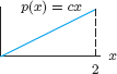
In Problems 9–12, calculate the value of c if p is a density function.
9.

10.

11.

12.
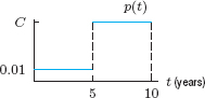
13. A machine lasts up to 10 years. Figure 7.7 shows the density function, p(t), for the length of time it lasts.
(a) What is the value of C?
(b) Is a machine more likely to break in its first year or in its tenth year? In its first or second year?
(c) What fraction of the machines lasts 2 years or less? Between 5 and 7 years? Between 3 and 6 years?
14. Find a density function p(x) such that p(x) = 0 when x ≥ 5 and when x < 0, and is decreasing when 0 ≤ x ≤ 5.
In Problems 15–17, graph a possible density function representing crop yield (in kilograms) from a field under the given circumstance.
15. All yields from 0 to 100 kg are equally likely; the field never yields more than 100 kg.
16. High yields are more likely than low. The maximum yield is 200 kg.
17. A drought makes low yields most common, and there is no yield greater than 30 kg.
18. Which of the following functions makes the most sense as a model for the probability density representing the time (in minutes, starting from t = 0) that the next customer walks into a store?

7.2 CUMULATIVE DISTRIBUTION FUNCTIONS AND PROBABILITY
Section 7.1 introduced density functions which describe the way in which a numerical characteristic is distributed through a population. In this section we study another way to present the same information.
Cumulative Distribution Function for Ages
An alternative way of showing how ages are distributed in the US is by using the cumulative distribution function P(t), defined by
![]()
Thus, P is the antiderivative of p with P(0) = 0, so P(t) is the area under the density curve between 0 and t. See the left-hand part of Figure 7.8.
Notice that the cumulative distribution function is nonnegative and increasing (or at least nondecreasing), since the number of people younger than age t increases as t increases. Another way of seeing this is to notice that P′ = p, and p is positive (or nonnegative). Thus the cumulative age distribution is a function which starts with P(0) = 0 and increases as t increases. We have P(t) = 0 for t < 0 because, when t < 0, there is no one whose age is less than t. The limiting value of P, as t → ∞, is 1 since as t becomes very large (100 say), everyone is younger than age t, so the fraction of people with age less than t tends toward 1.
We want to find the cumulative distribution function for the age density function shown in Figure 7.3. We see that P(10) is equal to 0.14, since Figure 7.3 shows that 14% of the population is between 0 and 10 years of age. Also,
![]()
and similarly
![]()
Continuing in this way gives the values for P(t) in Table 7.3. These values were used to graph P(t) in the right-hand part of Figure 7.8.
Table 7.3 Cumulative distribution function, P(t), giving fraction of US population of age less than t years
![]()

Figure 7.8: Graph of p(x), the age density function, and its relation to P(t), the cumulative age distribution function
Cumulative Distribution Function
A cumulative distribution function, P(t), of a density function p, is defined by

Thus, P is an antiderivative of p, that is, P′ = p.
Any cumulative distribution function has the following properties:
- P is increasing (or nondecreasing).


| Example 1 | The time to conduct a routine maintenance check on a machine has a cumulative distribution function P(t), which gives the fraction of maintenance checks completed in time less than or equal to t minutes. Values of P(t) are given in Table 7.4.
(a) What fraction of maintenance checks are completed in 15 minutes or less? (b) What fraction of maintenance checks take longer than 30 minutes? (c) What fraction take between 10 and 15 minutes? (d) Draw a histogram showing how times for maintenance checks are distributed. (e) In which of the given 5-minute intervals is the length of a maintenance check most likely to fall? (f) Give a rough sketch of the density function. (g) Sketch a graph of the cumulative distribution function. |
| Solution | (a) The fraction of maintenance checks completed in 15 minutes is P(15) = 0.21, or 21%.
(b) Since P(30) = 0.98, we see that 98% of maintenance checks take 30 minutes or less. Therefore, only 2% take more than 30 minutes. (c) Since 8% take 10 minutes or less and 21% take 15 minutes or less, the fraction taking between 10 and 15 minutes is 0.21 − 0.08 = 0.13, or 13%. (d) We begin by making a table showing how the times are distributed. Table 7.4 shows that the fraction of checks completed between 0 and 5 minutes is 0.03, and the fraction completed between 5 and 10 minutes is 0.05, and so on. See Table 7.5. The histogram in Figure 7.9 is drawn so that the area of each bar is the fraction of checks completed in the corresponding time period. For instance, the first bar has area 0.03 and width 5 minutes, so its height is 0.03/5 = 0.006.
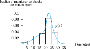
Figure 7.9: Histogram of times for maintenance checks (e) From Figure 7.9, we see that more of the checks take between 20 and 25 minutes to complete, so this is the most likely length of time. (f) The density function, p(t), is a smoothed version of the histogram in Figure 7.9. A reasonable sketch is given in Figure 7.10. (g) A graph of P(t) is given in Figure 7.11. Since P(t) is a cumulative distribution function, P(t) is approaching 1 as t gets large, but is never larger than 1.
Figure 7.10: Density function for time to conduct maintenance checks
Figure 7.11: Cumulative distribution function for time to conduct maintenance checks |


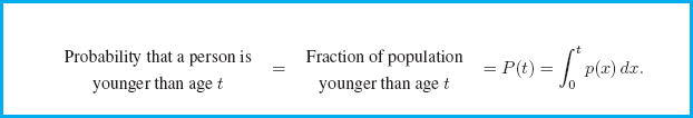
Probability
Suppose we pick a member of the US population at random. What is the probability that we pick a person who is between, say, the ages of 70 and 80? We saw in Table 7.2 on page 333 that 6% of the population is in this age group. We say that the probability, or chance, that the person is between 70 and 80 is 0.06. Using any age density function p(t), we define probabilities as follows:

Since the cumulative distribution gives the fraction of the population younger than age t, the cumulative distribution function can also be used to calculate the probability that a randomly selected person is in a given age group.
In the next example, both a density function and a cumulative distribution function are used to describe the same situation.
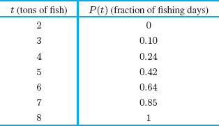
| Example 2 | Suppose you want to analyze the fishing industry in a small town. Each day, the boats bring back at least 2 tons of fish, but never more than 8 tons.
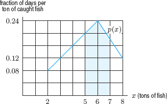
(a) Using the density function describing the daily catch in Figure 7.12, find and graph the corresponding cumulative distribution function and explain its meaning. (b) What is the probability that the catch is between 5 and 7 tons?
|
| Solution | (a) The cumulative distribution function P(t) is equal to the fraction of days on which the catch is less than t tons of fish. Since the catch is never less than 2 tons, we have P(t) = 0 for t ≤ 2. Since the catch is always less than 8 tons, we have P(t) = 1 for t ≥ 8. For t in the range 2 < t < 8 we must evaluate the integral
This integral equals the area under the graph of p(x) between x = 2 and x = t. It can be computed by counting grid squares in Figure 7.12; each square has area 0.04. For example,
Table 7.6 contains values of P(t); the graph is shown in Figure 7.13. Table 7.6 Estimates for P(t) of daily catch
Figure 7.13: Cumulative distribution, P(t), of daily catch (b) The probability that the catch is between 5 and 7 tons can be found using either the density function p or the cumulative distribution function P. When we use the density function, this probability is represented by the shaded area in Figure 7.14, which is about 10.75 squares, so
The probability can be found from the cumulative distribution function as follows:
Figure 7.14: Shaded area represents the probability the catch is between 5 and 7 tons |


Problems for Section 7.2
1. (a) Using the density function in Example 2 on page 334, fill in values for the cumulative distribution function P(t) for the length of time people wait in the doctor's office.
![]()
(b) Graph P(t).
2. Show that the area under the fishing density function in Figure 7.12 on page 339 is 1. Why is this to be expected?
3. Figure 7.15 shows a density function and the corresponding cumulative distribution function.5
(a) Which curve represents the density function and which represents the cumulative distribution function? Give a reason for your choice.
(b) Put reasonable values on the tick marks on each of the axes.

4. In an agricultural experiment, the quantity of grain from a given size field is measured. The yield can be anything from 0 kg to 50 kg. For each of the following situations, pick the graph that best represents the:
(i) Probability density function
(ii) Cumulative distribution function.
(a) Low yields are more likely than high yields.
(b) All yields are equally likely.
(c) High yields are more likely than low yields.
(I)

(II)

(III)

(IV)

(V)

(VI)

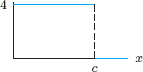
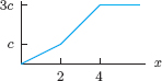
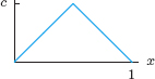
Decide if the function graphed in Problems 5–10 is a probability density function (pdf) or a cumulative distribution function (cdf). Give reasons. Find the value of c. Sketch and label the other function. (That is, sketch and label the cdf if the problem shows a pdf, and the pdf if the problem shows a cdf.)
5.
6.

7.

8.

9.
10.
11. A person who travels regularly on the 9:00 am bus from Oakland to San Francisco reports that the bus is almost always a few minutes late but rarely more than five minutes late. The bus is never more than two minutes early, although it is on very rare occasions a little early.
(a) Sketch a density function, p(t), where t is the number of minutes that the bus is late. Shade the region under the graph between t = 2 minutes and t = 4 minutes. Explain what this region represents.
(b) Now sketch the cumulative distribution function P(t). What measurement(s) on this graph correspond to the area shaded? What do the inflection point(s) on your graph of P correspond to on the graph of p? Interpret the inflection points on the graph of P without referring to the graph of p.
12. Suppose F(x) is the cumulative distribution function for heights (in meters) of trees in a forest.
(a) Explain in terms of trees the meaning of the statement F(7) = 0.6.
(b) Which is greater, F(6) or F(7)? Justify your answer in terms of trees.
13. Students at the University of California were surveyed and asked their grade point average. (The GPA ranges from 0 to 4, where 2 is just passing.) The distribution of GPAs is shown in Figure 7.16.6
(a) Roughly what fraction of students are passing?
(b) Roughly what fraction of the students have honor grades (GPAs above 3)?
(c) Why do you think there is a peak around 2?
(d) Sketch the cumulative distribution function.

14. The density function and cumulative distribution function of heights of grass plants in a meadow are in Figures 7.17 and 7.18, respectively.
(a) There are two species of grass in the meadow, a short grass and a tall grass. Explain how the graph of the density function reflects this fact.
(b) Explain how the graph of the cumulative distribution function reflects the fact that there are two species of grass in the meadow.
(c) About what percentage of the grasses in the meadow belong to the short grass species?


15. A congressional committee is investigating a defense contractor whose projects often incur cost overruns. The data in Table 7.7 show y, the fraction of the projects with an overrun of at most C%.
(a) Plot the data with C on the horizontal axis. Is this a density function or a cumulative distribution function? Sketch a curve through these points.
(b) If you think you drew a density function in part (a), sketch the corresponding cumulative distribution function on another set of axes. If you think you drew a cumulative distribution function in part (a), sketch the corresponding density function.
(c) Based on the table, what is the probability that there will be a cost overrun of 50% or more? Between 20% and 50%? Near what percent is the cost overrun most likely to be?
Table 7.7 Fraction, y, of overruns that are at most C%
![]()
For Problems 16–17, let p(t) = −0.0375t2 + 0.225t be the density function for the shelf life of a brand of banana, with t in weeks and 0 ≤ t ≤ 4. See Figure 7.19.

16. Find the probability that a banana will last
(a) Between 1 and 2 weeks.
(b) More than 3 weeks.
(c) More than 4 weeks.
17. (a) Sketch the cumulative distribution function for the shelf life of bananas. [Note: The domain of your function should be all real numbers, including to the left of t = 0 and to the right of t = 4.]
(b) Use the cumulative distribution function to estimate the probability that a banana lasts between 1 and 2 weeks. Check with Problem 16(a).
18. An experiment is done to determine the effect of two new fertilizers A and B on the growth of a species of peas. The cumulative distribution functions of the heights of the mature peas without treatment and treated with each of A and B are graphed in Figure 7.20.
(a) About what height are most of the unfertilized plants?
(b) Explain in words the effect of the fertilizers A and B on the mature height of the plants.

19. A group of people have received treatment for cancer. Let t be the survival time, the number of years a person lives after the treatment. The density function giving the distribution of t is p(t) = Ce−Ct for some positive constant C. What is the practical meaning of the cumulative distribution function P(t) = ![]() ?
?
20. The probability of a transistor failing between t = a months and t = b months is given by ![]() , for some constant c.
, for some constant c.
(a) If the probability of failure within the first six months is 10%, what is c?
(b) Given the value of c in part (a), what is the probability the transistor fails within the second six months?
21. While taking a walk along the road where you live, you accidentally drop your glove, but you don't know where. The probability density p(x) for having dropped the glove x kilometers from home (along the road) is
![]()
(a) What is the probability that you dropped it within 1 kilometer of home?
(b) At what distance y from home is the probability that you dropped it within y km of home equal to 0.95?
7.3 THE MEDIAN AND THE MEAN
It is often useful to be able to give an “average” value for a distribution. Two measures that are in common use are the median and the mean.
The Median
A median of a quantity x distributed through a population is a value T such that half the population has values of x less than (or equal to) T, and half the population has values of x greater than (or equal to) T. Thus, if p is the density function, a median T satisfies
![]()
In other words, half the area under the graph of p lies to the left of T. Equivalently, if P is the cumulative distribution function,
![]()
| Example 1 | Let t days be the length of time a pair of jeans remains in a shop before it is sold. The density function of t is graphed in Figure 7.21 and given by
(a) What is the longest time a pair of jeans remains unsold? (b) Would you expect the median time till sale to be less than, equal to, or greater than 25 days? (c) Find the median time required to sell a pair of jeans.
Figure 7.21: Density function for time till sale of a pair of jeans |
| Solution | (a) The density function is 0 for all times t > 50, so all jeans are sold within 50 days.
(b) The area under the graph of the density function in the interval 0 ≤ t ≤ 25 is greater than the area under the graph in the interval 25 ≤ t ≤ 50. So more than half the jeans are sold before their 25th day in the shop. The median time till sale is less than 25 days. (c) Let P be the cumulative distribution function. We want to find the value of T such that
Using a calculator to evaluate the integrals, we obtain the values for P in Table 7.8. Table 7.8 Cumulative distribution for selling time
Since about half the jeans are sold within 15 days, the median time to sale is about 15 days. See Figures 7.22 and 7.23. We could also use the Fundamental Theorem of Calculus to find the median exactly. See Problem 19. |


Figure 7.22: Median and density function

The Mean
Another commonly used average value is the mean. To find the mean of N numbers, we add the numbers and divide the sum by N. For example, the mean of the numbers 1, 2, 7, and 10 is (1 + 2 + 7 + 10)/4 = 5. The mean age of the entire US population is therefore defined as
![]()
Calculating the sum of all the ages directly would be an enormous task; we approximate the sum by an integral. We consider the people whose age is between t and t + Δt. How many are there?
The fraction of the population with age between t and t + Δt is the area under the graph of p between these points, which is approximated by the area of the rectangle, p(t)Δt. (See Figure 7.24.) If the total number of people in the population is N, then
![]()
The age of each of these people is approximately t, so
![]()

Figure 7.24: Shaded area is percentage of population with age between t and t + Δt
Therefore, adding and factoring out an N gives us
![]()
In the limit, as Δt shrinks to 0, the sum becomes an integral. Assuming no one is over 100 years old, we have
![]()
Since N is the total number of people in the US,
![]()
We can give the same argument for any7 density function p(x).
If a quantity has density function p(x),
![]()
It can be shown that the mean is the point on the horizontal axis where the region under the graph of the density function, if it were made out of cardboard, would balance.
| Example 2 | Find the mean time for jeans sales, using the density function of Example 1. |
| Solution | The formula for p is p(t) = 0.04 − 0.0008t. We compute
The mean is represented by the balance point in Figure 7.25. Notice that the mean is different from the median computed in Example 1. |

Normal Distributions
How much rain do you expect to fall in your home town this year? If you live in Anchorage, Alaska, the answer is something close to 15 inches (including the snow). Of course, you don't expect exactly 15 inches. Some years there are more than 15 inches, and some years there are less. Most years, however, the amount of rainfall is close to 15 inches; only rarely is it well above or well below 15 inches. What does the density function for the rainfall look like? To answer this question, we look at rainfall data over many years. Records show that the distribution of rainfall is well approximated by a normal distribution. The graph of its density function is a bell-shaped curve which peaks at 15 inches and slopes downward approximately symmetrically on either side.
Normal distributions are frequently used to model real phenomena, from grades on an exam to the number of airline passengers on a particular flight. A normal distribution is characterized by its mean, μ, and its standard deviation, α. The mean tells us the location of the central peak. The standard deviation tells us how closely the data is clustered around the mean. A small value of α tells us that the data is close to the mean; a large α tells us the data is spread out. In the following formula for a normal distribution, the factor of ![]() makes the area under the graph equal to 1.
makes the area under the graph equal to 1.
A normal distribution has a density function of the form
![]()
where μ is the mean of the distribution and σ is the standard deviation, with σ > 0.
To model the rainfall in Anchorage, we use a normal distribution with μ = 15 and σ = 1. (See Figure 7.26.)

Figure 7.26: Normal distribution with μ = 15 and σ = 1
Among the normal distributions, the one having μ = 0, σ = 1 is called the standard normal distribution. Values of the corresponding cumulative distribution function are published in tables.
Problems for Section 7.3
1. Estimate the median daily catch for the fishing data given in Example 2 of Section 7.2.
2. (a) Use the cumulative distribution function in Figure 7.27 to estimate the median.
(b) Describe the density function: For what values is it positive? Increasing? Decreasing? Identify all local maxima and minima values.

3. A quantity x is distributed with density function p(x) = 0.5(2 − x) for 0 ≤ x ≤ 2 and p(x) = 0 otherwise. Find the mean and median of x.
4. A quantity x has cumulative distribution function P(x) = x − x2/4 for 0 ≤ x ≤ 2 and P(x) = 0 for x < 0 and P(x) = 1 for x > 2. Find the mean and median of x.
For Problems 5–6, let p(t) = −0.0375t2+0.225t be the density function for the shelf life of a brand of banana which lasts up to 4 weeks. Time, t, is measured in weeks and 0 ≤ t ≤ 4.
5. Find the median shelf life of a banana using p(t). Plot the median on a graph of p(t). Does it look like half the area is to the right of the median and half the area is to the left?
6. Find the mean shelf life of a banana using p(t). Plot the mean on a graph of p(t). Does it look like the mean is the place where the density function balances?
7. Suppose that x measures the time (in hours) it takes for a student to complete an exam. All students are done within two hours and the density function for x is
![]()
(a) What proportion of students take between 1.5 and 2.0 hours to finish the exam?
(b) What is the mean time for students to complete the exam?
(c) Compute the median of this distribution.
8. Let p(t) = 0.1e−0.1t be the density function for the waiting time at a subway stop, with t in minutes, 0 ≤ t ≤ 60.
(a) Graph p(t). Use the graph to estimate visually the median and the mean.
(b) Calculate the median and the mean. Plot both on the graph of p(t).
(c) Interpret the median and mean in terms of waiting time.
9. The speeds of cars on a road are approximately normally distributed with a mean μ = 58 km/hr and standard deviation σ = 4 km/hr.
(a) What is the probability that a randomly selected car is going between 60 and 65 km/hr?
(b) What fraction of all cars are going slower than 52 km/hr?
10. The distribution of IQ scores can be modeled by a normal distribution with mean 100 and standard deviation 15.
(a) Write the formula for the density function of IQ scores.
(b) Estimate the fraction of the population with IQ between 115 and 120.
11. Let P(x) be the cumulative distribution function for the household income distribution in the US in 2009.8 Values of P(x) are in the following table:
![]()
(a) What percent of the households made between $40,000 and $60,000? More than $100,000?
(b) Approximately what was the median income?
(c) Is the statement “More than one-third of households made between $40,000 and $75,000” true or false?
CHAPTER SUMMARY
- Density function
- Cumulative distribution function
- Probability
- Median
- Mean
- Normal distribution
REVIEW PROBLEMS FOR CHAPTER SEVEN
In Problems 1–4, given that p(x) is a density function, find the value of (a).
1.

2.

3.

4.

In Problems 5–6, graph a density function representing the given distribution.
5. The age at which a person dies in a society with high infant mortality and in which adults usually die between age 40 and age 60.
6. The heights of the people in an elementary school.
7. Match the graphs of the density functions (a), (b), and (c) with the graphs of the cumulative distribution functions I, II, and III.

In Problems 8–10, graph a density function and a cumulative distribution function which could represent the distribution of income through a population with the given characteristics.
8. A large middle class.
9. Small middle and upper classes and many poor people.
10. Small middle class, many poor and many rich people.
11. An insect has a life-span of no more than one year. Figure 7.28 shows the density function, p(t), for the lifespan.
(a) Do more insects die in the first month of their life or the twelfth month of their life?
(b) What fraction of the insects live no more than 6 months?
(c) What fraction of the insects live more than 9 months?

12. A large number of people take a standardized test, receiving scores described by the density function p graphed in Figure 7.29. Does the density function imply that most people receive a score near 50? Explain why or why not.

13. Figure 7.30 shows the distribution of the number of years of education completed by adults in a population. What does the shape of the graph tell you? Estimate the percentage of adults who have completed less than 10 years of education.

14. Figure 7.31 shows P(t), the percentage of inventory of an item that has sold by time t, where t is in days and day 1 is January 1.
(a) When did the first item sell? The last item?
(b) On May 1 (day 121), what percentage of the inventory had been sold?
(c) Approximately what percentage of the inventory sold during May and June (days 121–181)?
(d) What percentage of the inventory remained after half of the year had passed (at day 181)?
(e) Estimate when items went on sale and sold quickly.

15. The density function for radii r (mm) of spherical raindrops during a storm is constant over the range 0 < r < 5 and zero elsewhere.
(a) Find the density function f(r) for the radii.
(b) Find the cumulative distribution function F(r).
16. Major absorption differences have been reported for different commercial versions of the same drug. One study compared three commercial versions of timed-release theophylline capsules.9 A theophylline solution was included for comparison. Figure 7.32 shows the cumulative distribution functions P(t), which represent the fraction of the drug absorbed by time t. Which curve represents the solution? Compare absorption rates of the four versions of the drug.

17. In southern Switzerland, most rain falls in the spring and fall; summers and winters are relatively dry. Sketch possible graphs for the density function and the cumulative distribution function of the rain distribution over the course of one year. Put the date on the horizontal axis and fraction of the year's rainfall on the vertical axis.
18. After measuring the duration of many telephone calls, the telephone company found their data was well approximated by the density function p(x) = 0.4e−0.4x, where x is the duration of a call, in minutes.
(a) What percentage of calls last between 1 and 2 minutes?
(b) What percentage of calls last 1 minute or less?
(c) What percentage of calls last 3 minutes or more?
(d) Find the cumulative distribution function.
19. Find the median of the density function given by p(t) = 0.04 − 0.0008t for 0 ≤ t ≤ 50 using the Fundamental Theorem of Calculus.
20. In 1950 an experiment was done observing the time gaps between successive cars on the Arroyo Seco Freeway. The data10 show that, if x is time in seconds and 0 ≤ x ≤ 40, the density function of these time gaps is
![]()
Find the median and mean time gap. Interpret them in terms of cars on the freeway.
In Problems 21–25, a quantity x is distributed through a population with probability density function p(x) and cumulative distribution function P(x). Decide if each statement is true or false. Give an explanation for your answer.
21. If p(10) = 1/2, then half the population has x < 10.
22. If P(10) = 1/2, then half the population has x < 10.
23. If p(10) = 1/2, then the fraction of the population lying between x = 9.98 and x = 10.04 is about 0.03.
24. If p(10) = p(20), then none of the population has x values lying between 10 and 20.
25. If P(10) = P(20), then none of the population has x values lying between 10 and 20.
STRENGTHEN YOUR UNDERSTANDING
In Problems 1–30, indicate whether the statement is true or false.
1. If ![]() p(x) dx = 1 then p(x) is a density function.
p(x) dx = 1 then p(x) is a density function.
2. The function given by p(x) = 0.25 when 0 ≤ x ≤ 4 and p(x) = 0 when x < 0 or x > 4 is a density function.
3. If p(x) is a density function for the age in years of a population, then ![]() is the fraction of the population with ages between 0 and 10 years.
is the fraction of the population with ages between 0 and 10 years.
4. If p(t) is a density function for waiting times in minutes at a bank teller, then ![]() is the fraction of the people waiting in line for that teller who wait between 10 and 15 minutes.
is the fraction of the people waiting in line for that teller who wait between 10 and 15 minutes.
5. If p(x) is the density function for age in years of the US population, then ![]() .
.
6. If p(x) is the density function for age in years of a population, then p(50) is the fraction of the population exactly 50 years old.
7. If p(x) is the density function for age in years of a population, and p(10) = 0.014, then about 1.4 percent of the population have ages between 9.5 and 10.5 years.
8. If p(x) is a density function, then ![]() .
.
9. If p(x) is a density function, then ![]() ≤
≤ ![]() .
.
10. If p(x) is a density function, then it could never happen that ![]() .
.
11. A cumulative distribution function P(t) can never be decreasing.
12. If P(t) is the cumulative distribution function corresponding to the density function P(t), then p′ = P.
13. If P(t) is a cumulative distribution function for a population, then P(30) is the fraction of the population with values above 30.
14. If P(t) is a cumulative distribution function for a population, then P(20) − P(10) is the fraction of the population with values between 10 and 20.
15. If P(t) is a cumulative distribution function for a population, then P(30) − P(10) = P(20).
16. If P(t) is a cumulative distribution function for age in years of a population and P(10) = 0.5, then one half of the population is less than 10 years old.
17. The units of a density function p(x) and its associated cumulative distribution function P(x) are the same.
18. A cumulative distribution function P(t) satisfies 0 ≤ P(t) ≤ 1 for all t.
19. If P(t) is a cumulative distribution function such that P(10) = 0.05 and P(15) = 0.08, then P(25) = 0.13.
20. If P(t) is the cumulative distribution function for a density function p(x), then P(50) − P(25) = ![]() .
.
21. If p(x) is the probability density function for a quantity, then the mean value of the quantity is ![]() .
.
22. If P(t) is the cumulative distribution function for a quantity, then the mean value of the quantity is given by ![]() .
.
23. If P(t) is the cumulative distribution function for a quantity, then the median value T of the quantity is given by T = P(0.5).
24. If p(x) is the density function for a quantity x, then the median T satisfies ![]()
25. If p(x) is the density function for a quantity x, then the median T satisfies ![]()
26. If a quantity has density function p(x), then the mean value and median are never equal.
27. The normal distribution with density function p(x) = ![]() has mean μ = 0 and standard deviation α = 1.
has mean μ = 0 and standard deviation α = 1.
28. The normal distribution with density function p(x) = ![]() has mean μ = −5 and standard deviation α = 1.
has mean μ = −5 and standard deviation α = 1.
29. The integral ![]() equals 1.
equals 1.
30. The mean value of a quantity x distributed through a population is the value T such that half of the population has values x less than or equal to T.
PROJECTS FOR CHAPTER SEVEN
1. Triangular Probability Distribution
Triangular probability distributions, such as the one with density function graphed in Figure 7.33, are used in business to model uncertainty. Such a distribution can be used to model a variable where only three pieces of information are available: a lower bound (x = a), a most likely value (x = c), and an upper bound (x = b).

Thus, we can write the function p(x) as two linear functions:
![]()
(a) Find the value of p(c) geometrically, using the criterion that the probability that x takes on some value between a and b is 1.
Suppose a new product costs between $6 and $10 per unit to produce, with a most likely cost of $9.
(b) Find p(9).
(c) Use the fact that p(6) = p(10) = 0 and the value of p(9) you found in part (b) to find m1, m2, b1, and b2.
(d) What is the probability that the production cost per unit will be less than $8?
(e) What is the median cost?
(f) Write a formula for the cumulative probability distribution function P(x) for
(i) 6 ≤ x ≤ 9,
(ii) 9 ≤ x ≤ 10.
Sketch the graph of P(x).
1www.censusscope.org/us/chart_age.html, accessed May 10. 2005.
2There are other types of histograms which have frequency on the vertical axis.
3In fact, 0.02% of the population is over 100, but this is too small to be visible on the histogram.
4Adapted from Statistics, 2nd Edition, by D. Freedman, R. Pisani, R. Purves, and A. Adikhari (New York: Norton, 1991).
5Adapted from Calculus, by David A. Smith and Lawrence C. Moore (Lexington, D.C. Heath, 1994).
6Adapted from Statistics, by Freedman, Pisani, Purves, and Adikhari (New York: Norton, 1991).
7Provided all the relevant improper integrals converge.
8http://www.census.gov/hhes/www/income/income.html, accessed January 7, 2012.
9Progress in Drug Metabolism, Bridges and Chasseaud (eds.) (New York: Wiley, 1980).
10Reported by Daniel Furlough and Frank Barnes.