

Chapter Six
ANTIDERIVATIVES AND APPLICATIONS
Contents
6.1 Analyzing Antiderivatives Graphically and Numerically
6.2 Antiderivatives and the Indefinite Integral
Finding Formulas for Antiderivatives
Antiderivatives of Periodic Functions
6.3 Using The Fundamental Theorem to Find Definite Integrals
6.4 Application: Consumer and Producer Surplus
6.5 Application: Present and Future Value
Present and Future Values of an Income Stream
6.6 Integration by Substitution
Using Substitution with Periodic Functions
Definite Integrals by Substitution
PROJECTS: Quabbin Reservoir, Distribution of Resources, Yield from an Apple Orchard
6.1 ANALYZING ANTIDERIVATIVES GRAPHICALLY AND NUMERICALLY
What is an Antiderivative?
If the derivative of F(x) is f(x), that is, if F′(x) = f(x), then we call F(x) an antiderivative of f (x). For example, the derivative of x2 is 2x, so we say that
![]()
In this section, we see how values of an antiderivative, F, are computed using the Fundamental Theorem of Calculus when the derivative, F′, and one value of the function, F(a), are known.
| Example 1 | Suppose F′ (t) = (1.8)t and F(0) = 2. Find the value of F(b) for b = 0, 0.1, 0.2,..., 1.0. |
| Solution | We apply the Fundamental Theorem with F′(t) = (1.8)t and a = 0 to get values for F(b):
Since F(0) = 2, we have
We use a calculator or computer to estimate the definite integral |


Table 6.1 Approximate values of F
![]()
Notice from the table that values of F(b) increase between b = 0 and b = 1. This is because the derivative F′(t) = (1.8)t is positive for t between 0 and 1.
Graphing an Antiderivative
To graph an antiderivative of F from its derivative F′ = f we can calculate values of F, as in Example 1, or we can use the graph of f and the following results from Section 2.2, page 99.
Suppose F is an antiderivative of f:
If f > 0 on an interval, then F is increasing on that interval.
If f < 0 on an interval, then F is decreasing on that interval.
If f = 0 on an interval, then F is constant on that interval.
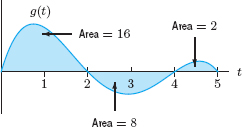
| Example 2 | Figure 6.1 shows the derivative f′(x) of a function f(x) and the values of some areas. If f(0) = 10, sketch a graph of the function f(x). Give the coordinates of the local maxima and minima.
|
| Solution | Figure 6.1 shows that the derivative f′ is positive between 0 and 2, negative between 2 and 5, and positive between 5 and 6. Therefore, the function f is increasing between 0 and 2, decreasing between 2 and 5, and increasing between 5 and 6. (See Figure 6.2.) There is a local maximum at x = 2 and a local minimum at x = 5.
Notice that we can sketch the general shape of the graph of f in Figure 6.2 without knowing any of the areas in Figure 6.1. The areas are used to make the graph more precise. We are told that f(0) = 10, so we plot the point (0, 10) on the graph of f in Figure 6.3. The Fundamental Theorem and Figure 6.1 show that
Therefore, the total change in f between x = 0 and x = 2 is 14. Since f(0) = 10, we have
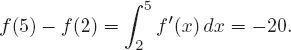
The point (2, 24) is on the graph of f. See Figure 6.3. Figure 6.1 shows that the area between x = 2 and x = 5 is 20. Since this area lies entirely below the x-axis, the Fundamental Theorem gives
The total change in f is −20 between x = 2 and x = 5. Since f(2) = 24, we have
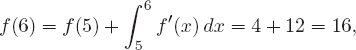
Thus, the point (5, 4) lies on the graph of f. Finally,
so the point (6, 16) is on the graph of f.
|


Concavity
If F is an antiderivative of f, then F″ = f′. Thus, we can determine the concavity of the graph of F from the properties of f′ (see Section 2.4, on page 113).
Suppose F is an antiderivative of f:
If f′ > 0 on an interval, then f is increasing and the graph of F is concave up on that interval.
If f′ < 0 on an interval, then f is decreasing and the graph of F is concave down on that interval.
Thus, inflection points of F occur where f changes from increasing to decreasing or vice versa.
Problems for Section 6.1
1. Suppose F′(x) = 2x2 + 5 and F(0) = 3. Find the value of F(b) for b = 0, 0.1, 0.2, 0.5, and 1.0.
2. Suppose G′(t) = (1.12)t and G(5) = 1. Find the value of G(b) for b = 5, 5.1, 5.2, 5.5, and 6.0.
3. Suppose f′(t) = (0.82)t and f(2) = 9. Find the value of f (b) for b = 2, 4, 6, 10, and 20.
4. (a) Using Figure 6.4, estimate ![]() f(x)dx.
f(x)dx.
(b) If F is an antiderivative of the same function f and F(0) = 25, estimate F(7).

5. Figure 6.5 shows f. If F′ = f and F(0) = 0, find F(b) for b = 1,2, 3, 4, 5, 6.

6. Figure 6.6 shows the derivative g′. If g(0) = 0, graph g. Give (x,y)-coordinates of all local maxima and minima.

7. The derivative F′(t) is graphed in Figure 6.7. Given that F(0) = 5, calculate F(t) for t = 1, 2, 3, 4, 5.

In Problems 8–13, sketch two functions F such that F′ = f.
In one case let F(0) = 0 and in the other, let F(0) = 1.
8.

9.

10.

11.

12.

13.

14. Figure 6.8 shows the derivative F′ of a function F. If F(20) = 150, estimate the maximum value attained by F.

15. Figure 6.9 shows the rate of change of the concentration of adrenaline, in micrograms per milliliter per minute, in a person's body. Sketch a graph of the concentration of adrenaline, in micrograms per milliliter, in the body as a function of time, in minutes.

16. Urologists are physicians who specialize in the health of the bladder. In a common diagnostic test, urologists monitor the emptying of the bladder using a device that produces two graphs. In one of the graphs the flow rate (in milliliters per second) is measured as a function of time (in seconds). In the other graph, the volume emptied from the bladder is measured (in milliliters) as a function of time (in seconds). See Figure 6.10.
(a) Which graph is the flow rate and which is the volume?
(b) Which one of these graphs is an antiderivative of the other?

17. Figure 6.11 shows the derivative F′ of F. Let F(0) = 0. Of the four numbers F(1), F(2), F(3), and F(4), which is largest? Which is smallest? How many of these numbers are negative?

Problems 18–19 show the derivative f′ of f.
(a) Where is f increasing and where is f decreasing? What are the x-coordinates of the local maxima and minima of f?
(b) Sketch a possible graph for f. (You don't need a scale on the vertical axis.)
18.

19.

20. During photosynthesis, plants absorb sunlight and release oxygen. The rate at which a leaf releases oxygen, the rate of photosynthesis, is a function of the age of the leaf. Figure 6.12 shows the rate of photosynthesis for a soybean leaf.1
(a) Sketch a graph of the amount of oxygen, E(t), generated by this leaf during the first 20 days of life.
(b) Give the t-coordinate of the inflection point in your sketch and interpret what this point tells you about soybean leaves and oxygen.
(c) Give a symbolic expression that represents the total amount of oxygen released by this leaf in its first 10 days of life.
(d) Does the soybean leaf release more oxygen during the first 10 days of its life or during the second 10 days of its life?

21. Using Figure 6.13, sketch a graph of an antiderivative G(t) of g(t) satisfying G(0) = 5. Label each critical point of G(t) with its coordinates.
22. Use Figure 6.14 and the fact that F(2) = 3 to sketch the graph of F(x). Label the values of at least four points.

23. Figure 6.15 shows the derivative F′. If F(0) = 14, graph F. Give (x, y)-coordinates of all local maxima and minima.

24. Figure 6.16 shows the derivative F′(t). If F(0) = 3, find the values of F(2), F(5), F(6). Graph F(t).

In Problems 25–26, a graph of f is given. Let F′(x) = f(x).
(a) What are the x-coordinates of the critical points of F(x)?
(b) Which critical points are local maxima, which are local minima, and which are neither?
(c) Sketch a possible graph of F(x).
25.

26.

Problems 27–28 concern the graph of f′ in Figure 6.17.

Figure 6.17: Note: Graph of f′, not f
27. Which is greater, f(0) or f(1)?
28. List the following in increasing order:
![]()
For Problems 29–32, show the following quantities on Figure 6.18.

29. A length representing f(b) − f(a).
30. A slope representing ![]()
31. An area representing F(b) − F(a), where F′ = f.
32. A length roughly approximating
![]()
6.2 ANTIDERIVATIVES AND THE INDEFINITE INTEGRAL
In the previous section we defined an antiderivative of a function f(x) to be a function F(x) whose derivative is f(x). For example, an antiderivative of 2x is F(x) = x2. Can you think of another function whose derivative is 2x? How about x2 + 1? Or x2 + 17? Since, for any constant C,
![]()
any function of the form x2 + C is an antiderivative of 2x. It can be shown that all antiderivatives of 2x are of this form, so we say that
![]()
Once we know one antiderivative F(x) for a function f(x) on an interval, then all other antiderivatives of f(x) are of the form F(x) + C.
The Indefinite Integral
We introduce a notation for the family of antiderivatives that looks like a definite integral without the limits. We call ∫ f(x)dx the indefinite integral of f(x). If all antiderivatives of f(x) are of the form F(x) + C, we write
![]()
It is important to understand the difference between

The first is a number and the second is a family of functions. Because the notation is similar, the word “integration” is frequently used for the process of finding antiderivatives as well as of finding definite integrals. The context usually makes clear which is intended.
| Example 1 | (a) Decide which functions are antiderivatives of f(x) = 8x3
(b) Find |
| Solution | (a) An antiderivative of 8x3 is any function whose derivative is 8x3. We have:
Since H′(x) = 8x3, the function H(x) is an antiderivative of 8x3. The two functions F(x) and G(x) are not antiderivatives of 8x3. (b) Since H(x) = 2x4 is one antiderivative of f(x), all other antiderivatives of f(x) are of the form H(x) + C. Thus,
|
Finding Formulas for Antiderivatives
Finding antiderivatives of functions is like taking square roots of numbers: if we pick a number at random, such as 7 or 493, we may have trouble figuring out its square root without a calculator. But if we happen to pick a number such as 25 or 64, which we know is a perfect square, then we can easily guess its square root. Similarly, if we pick a function which we recognize as a derivative, then we can find its antiderivative easily.
For example, noticing that 2x is the derivative of x2 tells us that x2 is an antiderivative of 2x. If we divide by 2, then we guess that
![]()
To check this statement, take the derivative of x2/2:

What about an antiderivative of x2? The derivative of x3 is 3x2, so the derivative of x3/3 is 3x2/3 = x2. Thus,
![]()
Can you see the pattern? It looks like
![]()
(We assume n ≠ −1, or we would have x0/0, which does not make sense.) It is easy to check this formula by differentiation:

Thus, in indefinite integral notation, we see that

Can you think of an antiderivative of the function f(x) = 5? We know that the derivative of 5x is 5, so F(x) = 5x is an antiderivative of f(x) = 5. In general, if k is a constant, the derivative of kx is k, so we have the result:
| Example 2 | Find ∫ (3x + x2) dx. |
| Solution | We know that x2/2 is an antiderivative of x and that x3/3 is an antiderivative of x2, so we expect
Again, we can check by differentiation:
|

The preceding example illustrates that the sum and constant multiplication rules of differentiation work in reverse:
Properties of Antiderivatives: Sums and Constant Multiples
In indefinite integral notation,
1. ![]()
2. ![]() .
.
In words,
1. An antiderivative of the sum (or difference) of two functions is the sum (or difference) of their antiderivatives.
2. An antiderivative of a constant times a function is the constant times an antiderivative of the function.
| Example 3 | Find all antiderivatives of each of the following: (a) x5 (b) t8 (c) 12x3 (d) q3 − 6q2 |
 |
|
| To check, differentiate the antiderivative; you should get the original function. | |
What is an antiderivative of xn when n = −1? In other words, what is an antiderivative of 1/x? Fortunately, we know a function whose derivative is 1/x, namely, the natural logarithm. Thus, since
![]()
we know that
![]()
If x < 0, then ln x is not defined, so it can't be an antiderivative of 1/x. In this case, we can try ln(−x):
![]()
so
![]()
This means ln x is an antiderivative of 1/x if x > 0, and ln(−x) is an antiderivative of 1/x if x < 0. Since |x| = x when x > 0 and |x| = −x when x < 0, we can collapse these two formulas into one. On any interval that does not contain 0,
Since the exponential function ex is its own derivative, it is also one of its own antiderivatives; thus
![]()
What about ekx? We know that the derivative of ekx is kekx, so, for k ≠ 0, we have

| Example 4 | Find all antiderivatives of each of the following: |
| Solution | |
Differentiate your answers to check them. |
Antiderivatives of Periodic Functions
Antiderivatives of the sine and cosine are easy to guess. Since
![]()
we get
![]()
Since the derivative of sin(kx) is k cos(kx) and the derivative of cos(kx) is −k sin(kx), we have, for k ≠ 0,

| Example 5 | Find |
| Solution | We break the antiderivative into two terms:
Check by differentiating:
|
Problems for Section 6.2
In Problems 1–6, decide if the function is an antiderivative of f(x) = 2e2x.
1. F(x) = e2x + 5
2. F(x) = e2x
3. F(x) = 5e2x
4. F(x) = xe2x
5. F(x) = 2e2x
6. ![]()
In Problems 7–13, decide whether the expression is a number or a family of functions. (Assume f(x) is a function.)
7. ![]()
8. ![]()
9. ![]()
10. ![]()
11. ![]()
12. ![]()
13. ![]()
In Problems 14–39, find an antiderivative.
14. f(t) = 5t
15. f(x) = x2
16. g(t) = t2 + t
17. f(x) = 5
18. f(x) = x4
19. g(t) = t7 + t3
20. f(q) = 5q2
21. g(x) = 6x3 + 4
22. h(y) = 3y2 −y3
23. k(x) = 10 + 8x3
24. p(r) = 2πr
25. f(x) = x + x5 + x−5
26. g(z) = ![]()
27. p(x) = x2 − 6x + 17
28. f(x) = 5x − ![]()
29. p(t) = t3 − ![]() − t
− t
30. r(t) = ![]()
31. g(z) = ![]()
32. f(z) = ez + 3
33. f(x) = x6 − ![]()
34. ![]()
35. ![]()
36. g(t) = e−3t
37. h(t) = cos t
38. g(t) = 5 + cos t
39. g(θ) = sin θ − 2 cos θ
In Problems 40–43 decide which function is an antiderivative of the other.
40. ![]()
41. f(x) = − sin x − cos x; g(x) = cos x − sin x
42. ![]()
43. ![]()
In Problems 44–49, find an antiderivative F(x) with F′(x) = f(x) and F(0) = 0. Is there only one possible solution?
44. f(x) = 3
45. f(x) = 2 + 4x + 5x2
46. f(x) = ![]()
47. f(x) = ![]()
48. f(x) = x2
49. f(x) = ex
In Problems 50–79, find the indefinite integrals.
50. ![]() (5x + 7)dx
(5x + 7)dx
51. ![]() 9x2 dx
9x2 dx
52. ![]() e−0.05t dt
e−0.05t dt
53. ![]()
54. ![]()
55. ![]()
56. ![]()
57. ![]() 5ez dz
5ez dz
58. ![]()
59. ![]()
60. ![]()
61. ![]() (x2 + 4x −5)dx
(x2 + 4x −5)dx
62. ![]() e2t dt
e2t dt
63. ![]()
64. ![]() (x3 + 5x2 + 6)dx
(x3 + 5x2 + 6)dx
65. ![]() (ex + 5)dx
(ex + 5)dx
66. ![]()
67. ![]()
68. ![]() e3r dr
e3r dr
69. ![]() sin t dt
sin t dt
70. ![]() 25e−0.04q dq
25e−0.04q dq
71. ![]() 100e4x dx
100e4x dx
72. ![]() cos θ dθ
cos θ dθ
73. ![]()
75. ![]() (3 cos x 7 sin x)dx
(3 cos x 7 sin x)dx
76. ![]() 6 cos(3 x)dx
6 cos(3 x)dx
77. ![]() (10 + 8 sin(2x))dx
(10 + 8 sin(2x))dx
78. ![]() (2ex − 8 cos x)dx
(2ex − 8 cos x)dx
79. ![]() (12 sin(2x) + 15 cos(5x))dx
(12 sin(2x) + 15 cos(5x))dx
In Problems 80–84 find an antiderivative and use differentiation to check your answer.
80. f(x) = ![]()
81. g(x) = ![]()
82. h(x) = ![]()
83. p(x) = e2x − e−2x
84. q(x) = 7sin x − sin7(x)
85. The marginal revenue function of a monopolistic producer is M R = 20 − 4q.
(a) Find the total revenue function.
(b) Find the corresponding demand curve.
86. A firm's marginal cost function is MC = 3q2 + 4q + 6. Find the total cost function if the fixed costs are 200.
− For Problems 87–90, find an antiderivative F(x) with F′(x) = f(x) and F(0) = 5.
87. f(x) = 6x − 5
88. f(x) = x2 + 1
89. f(x) = 8 sin(2x)
90. f(x) = 6e3x
91. In drilling an oil well, the total cost, C, consists of fixed costs (independent of the depth of the well) and marginal costs, which depend on depth; drilling becomes more expensive, per meter, deeper into the earth. Suppose the fixed costs are 1,000,000 riyals (the riyal is the unit of currency of Saudi Arabia), and the marginal costs are
C′(x) = 4000 + 10x riyals/meter,
where x is the depth in meters. Find the total cost of drilling a well x meters deep.
92. Over the past fifty years the carbon dioxide level in the atmosphere has increased. Carbon dioxide is believed to drive temperature, so predictions of future carbon dioxide levels are important. If C(t) is carbon dioxide level in parts per million (ppm) and t is time in years since 1950, three possible models are:2
I C′ (t) = 1.3
II C′ (t) = 0.5 + 0.03t
III C′ (t) = 0.5e0.02t
(a) Given that the carbon dioxide level was 311 ppm in 1950, find C(t) for each model.
(b) Find the carbon dioxide level in 2020 predicted by each model.
6.3 USING THE FUNDAMENTAL THEOREM TO FIND DEFINITE INTEGRALS
In the previous section we calculated antiderivatives. In this section we see how antiderivatives are used to calculate definite integrals exactly. This calculation is based on the Fundamental Theorem:
Fundamental Theorem of Calculus
If f is continuous on the interval [a, b] and F(x) is an antiderivative of f, that is if F′(x) = f(x)

So far we have approximated definite integrals using a graph or left- and right-hand sums. The Fundamental Theorem gives us another method of calculating definite integrals. To find ![]() we first try to find an antiderivative, F, of f(x) and then calculate F(b) − F(a). This method of computing definite integrals has an important advantage: it gives an exact answer. However, the method works only when we can find a formula for an antiderivative F(x). We must approximate definite integrals of functions such as f(x) = e−x2 where we can not find a formula for an antiderivative.
we first try to find an antiderivative, F, of f(x) and then calculate F(b) − F(a). This method of computing definite integrals has an important advantage: it gives an exact answer. However, the method works only when we can find a formula for an antiderivative F(x). We must approximate definite integrals of functions such as f(x) = e−x2 where we can not find a formula for an antiderivative.
 numerically and using the Fundamental Theorem.

In Example 1 we used the antiderivative F(x) = x2, but F(x) = x2 + C works just as well for any constant C, because the constant cancels out when we subtract F (a) from F (b):

It is helpful to introduce a shorthand notation for F (b) − F(a): we write

For example:

| Example 2 | Use the Fundamental Theorem to compute the following definite integrals:
|
| Solution | (a) Since f(x) = 6x2, we take F(x) = 6(x3/3) = 2x3. So
(b) Since f(t) = t3, we take F(x) = t4/4, So
(c) Since f(x) = 8x + 5, we take F(x) = 4x2 + 5x, giving
(d) Since f(t) = 8e2t, we take F(t) = (8e2t)/2 = 4e2t, so
|


| Example 3 | Write a definite integral to represent the area under the graph of f(t) = e0.5t between t = 0 and t = 4. Use the Fundamental Theorem to calculate the area. |
| Solution | The function is graphed in Figure 6.19. We have
|


Improper Integrals
So far, in our discussion of the definite integral  we have assumed that the interval a ≤ x ≤ b is of finite length and the integrand f is continuous. An improper integral is a definite integral in which one (or both) of the limits of integration is infinite or the integrand is unbounded. An example of an improper integral is
![]()
| Example 4 | Interpret and estimate the value of
|
| Solution | This integral represents the area under the graph of To estimate the value of the integral, we find the area under the curve between x = 1 and x = b, where b is large. The larger the value of b, the better the estimate. For example for b = 10,100,1000:
These calculations suggest that as the upper limit of integration tends to infinity, the estimates tend to 1.
|


We say that the improper integral ![]() converges to 1. To show that the integral converges to exactly 1 (and not to 1.0001, say), we need to use the Fundamental Theorem of Calculus. (See Problem 29.) It may seem surprising that the region shaded in Figure 6.20 (which has infinite length) can have finite area. The area is finite because the values of the function 1/x2 shrink to zero very fast as x → ∞. In other examples (where the integrand does not shrink to zero so fast), the area represented by an improper integral may not be finite. In that case, we say the improper integral diverges. (See Problem 43.)
converges to 1. To show that the integral converges to exactly 1 (and not to 1.0001, say), we need to use the Fundamental Theorem of Calculus. (See Problem 29.) It may seem surprising that the region shaded in Figure 6.20 (which has infinite length) can have finite area. The area is finite because the values of the function 1/x2 shrink to zero very fast as x → ∞. In other examples (where the integrand does not shrink to zero so fast), the area represented by an improper integral may not be finite. In that case, we say the improper integral diverges. (See Problem 43.)
Problems for Section 6.3
Using the Fundamental Theorem, evaluate the definite integrals in Problems 1–20 exactly.
1. 
2. 
3. 
4. 
5. ![]()
6. 
7. 
8. 
9. 
10. 
11. 
12. 
13. 
14. 
15. 
16. 
17. ![]()
18. 
19. 
20. 
21. Find the exact area of the region bounded by the x-axis and the graph of y = x3 − x.
22. Use the Fundamental Theorem of Calculus to find the average value of f(x) = e0.5x between x = 0 and x = 3. Show the average value on a graph of f(x).
23. Use the Fundamental Theorem to determine the value of b if the area under the graph of f(x) = x2 between x = 0 and x = b is equal to 100. Assume b > 0.
24. Use the Fundamental Theorem to determine the value of b if the area under the graph of f(x) = 4x between x = 1 and x = b is equal to 240. Assume b > 1.
25. If t is in years, and t = 0 is January 1, 2005, worldwide energy consumption, r, in quadrillion (1015) BTUs per year, is modeled by
![]()
(a) Write a definite integral for the total energy use between the start of 2005 and the start of 2010.
(b) Use the Fundamental Theorem of Calculus to evaluate the integral. Give units with your answer.
26. Oil is leaking out of a ruptured tanker at the rate of r(t) = 50e−0.02t thousand liters per minute.
(a) At what rate, in liters per minute, is oil leaking out at t = 0? At t = 60?
(b) How many liters leak out during the first hour?
27. (a) Between 2000 and 2010, ACME Widgets sold widgets at a continuous rate of R = R0e0.125t widgets per year, where t is time in years since January 1, 2000. Suppose they were selling widgets at a rate of 1000 per year on January 1, 2000. How many widgets did they sell between 2000 and 2010? How many did they sell if the rate on January 1, 2000 was 1,000,000 widgets per year?
(b) In the first case (1000 widgets per year on January 1, 2000), how long did it take for half the widgets in the ten-year period to be sold? In the second case (1,000,000 widgets per year on January 1, 2000), when had half the widgets in the ten-year period been sold?
(c) In 2010, ACME advertised that half the widgets it had sold in the previous ten years were still in use. Based on your answer to part (b), how long must a widget last in order to justify this claim?
28. Decide if the improper integral ![]() converges, and if so, to what value, by the following method.
converges, and if so, to what value, by the following method.
(a) Use a computer or calculator to find ![]() for b = 3, 5, 7, 10. What do you observe? Make a guess about the convergence of the improper integral.
for b = 3, 5, 7, 10. What do you observe? Make a guess about the convergence of the improper integral.
(b) Find ![]() using the Fundamental Theorem. Your answer will contain b.
using the Fundamental Theorem. Your answer will contain b.
(c) Take a limit as b → ∞. Does your answer confirm your guess?
29. In this problem, you will show that the following improper integral converges to 1:
![]()
(a) Use the Fundamental Theorem to find ![]() . Your answer will contain b.
. Your answer will contain b.
(b) Now take the limit as b → ∞. What does this tell you about the improper integral?
30. (a) Graph f(x) = e−x2 and shade the area represented by the improper integral ![]() .
.
(b) Use a calculator or computer to find ![]() for a = 1, a = 2, a = 3, a = 5.
for a = 1, a = 2, a = 3, a = 5.
(c) The improper integral ![]() converges to a finite value. Use your answers from part (b) to estimate that value.
converges to a finite value. Use your answers from part (b) to estimate that value.
31. Graph y = 1/x2 and y = 1/x3 on the same axes. Which do you think is larger: ![]() Why?
Why?
32. At a time t hours after taking a tablet, the rate at which a drug is being eliminated is
![]()
Assuming that all the drug is eventually eliminated, calculate the original dose.
33. The rate, r, at which people get sick during an epidemic of the flu can be approximated by
![]()
where r is measured in people/day and t is measured in days since the start of the epidemic.
(a) Write an improper integral representing the total number of people that get sick.
(b) Use a graph of r to represent the improper integral from part (a) as an area.
34. An island has a carrying capacity of 1 million rabbits. (That is, no more than 1 million rabbits can be supported by the island.) The rabbit population is two at time t = 1 day and grows at a rate of r(t) thousand rabbits/day until the carrying capacity is reached. For each of the following formulas for r(t), is the carrying capacity ever reached? Explain your answer.
(a) r(t) = 1/t2
(b) r(t) = t
(c) ![]()
6.4 APPLICATION: CONSUMER AND PRODUCER SURPLUS
Supply and Demand Curves
As we saw in Chapter 1, the quantity of a certain item produced and sold can be described by the supply and demand curves of the item. The supply curve shows what quantity, q, of the item the producers supply at different prices, p. The consumers' behavior is reflected in the demand curve, which shows what quantity of goods are bought at various prices. See Figure 6.21.

Figure 6.21: Supply and demand curves
It is assumed that the market settles at the equilibrium price p* and equilibrium quantity q* where the graphs cross. At equilibrium, a quantity q* of an item is produced and sold for a price of p* each.
Consumer and Producer Surplus
Notice that at equilibrium, a number of consumers have bought the item at a lower price than they would have been willing to pay. (For example, there are some consumers who would have been willing to pay prices up to p1.) Similarly, there are some suppliers who would have been willing to produce the item at a lower price (down to p0, in fact). We define the following terms:
- The consumer surplus measures the consumers' gain from trade. It is the total amount gained by consumers by buying the item at the current price rather than at the price they would have been willing to pay.
- The producer surplus measures the suppliers' gain from trade. It is the total amount gained by producers by selling at the current price, rather than at the price they would have been willing to accept.
In the absence of price controls, the current price is assumed to be the equilibrium price.
Both consumers and producers are richer for having traded. The consumer and producer surplus measure how much richer they are.

Figure 6.22: Calculation of consumer surplus
Suppose that all consumers buy the good at the maximum price they are willing to pay. Subdivide the interval from 0 to q* into intervals of length Δq. Figure 6.22 shows that a quantity Δq of items are sold at a price of about p1, another Δq are sold for a slightly lower price of about p2, the next Δq for a price of about p3, and so on. Thus, the consumers' total expenditure is about
![]()
If the demand curve has equation3 p = f (q), and if all consumers who were willing to pay more than p* paid as much as they were willing, then as Δq → 0, we would have
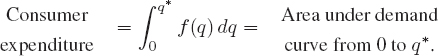
If all goods are sold at the equilibrium price, the consumers' actual expenditure is only p*q*, which is the area of the rectangle between the q-axis and the line p = p* from q = 0 to q = q*. The consumer surplus is the difference between the total consumer expenditure if all consumers pay the maximum they are willing to pay and the actual consumer expenditure if all consumers pay the current price. The consumer surplus is represented by the area in Figure 6.23. Similarly, the producer surplus is represented by the area in Figure 6.24. (See Problems 16 and 17.) Thus:


| Example 1 | The supply and demand curves for a product are given in Figure 6.25.
Figure 6.25: Supply and demand curves for a product (a) What are the equilibrium price and quantity? (b) At the equilibrium price, calculate and interpret the consumer and producer surplus. |
| Solution | (a) The equilibrium price is p* = $80 per unit and the equilibrium quantity is q* = 80,000 units.
(b) The consumer surplus is the area under the demand curve and above the line p = 80. (See Figure 6.26.) We have
This tells us that consumers gain $6,400,000 in buying goods at the equilibrium price instead of at the price they would have been willing to pay.
The producer surplus is the area above the supply curve and below the line p = 80. (See Figure 6.27.) We have
So, producers gain $3,200,000 by supplying goods at the equilibrium price instead of the price at which they would have been willing to provide the goods. |


Wage and Price Controls
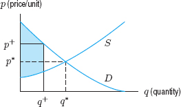
In a free market, the price of a product generally moves to the equilibrium price, unless outside forces keep the price artificially high or artificially low. Rent control, for example, keeps prices below market value, whereas cartel pricing or the minimum-wage law raise prices above market value. What happens to consumer and producer surplus at non-equilibrium prices?
| Example 2 | The dairy industry has cartel pricing: the government has set milk prices artificially high. What effect does raising the price to p+ from the equilibrium price have on:
(a) Consumer surplus? (b) Producer surplus? (c) Total gains from trade (that is, Consumer surplus + Producer surplus)?
Figure 6.28: What is the effect of the artificially high price, p+, on consumer and producer surplus? (q* and p* are equilibrium values) |
| Solution | (a) A graph of possible supply and demand curves for the milk industry is given in Figure 6.28. Suppose that the price is fixed at p+, above the equilibrium price. Consumer surplus is the difference between the amount the consumers paid (p+) and the amount they would have been willing to pay (given on the demand curve). This is the area shaded in Figure 6.29. This consumer surplus is less than the consumer surplus at the equilibrium price, shown in Figure 6.30.
Figure 6.29: Consumer surplus: Artificial price
Figure 6.30: Consumer surplus: Equilibrium price (b) At a price of p+, the quantity sold, q+, is less than it would have been at the equilibrium price. The producer surplus is represented by the area between p+ and the supply curve at this reduced demand. This area is shaded in Figure 6.31. Compare this producer surplus (at the artificially high price) to the producer surplus in Figure 6.32 (at the equilibrium price). In this case, producer surplus appears to be greater at the artificial price than at the equilibrium price. (However, different supply and demand curves might lead to a different answer.)
Figure 6.31: Producer surplus: Artificial price
Figure 6.32: Producer surplus: Equilibrium price (c) The total gains from trade (Consumer surplus + Producer surplus) at the price of p+ is represented by the area shaded in Figure 6.33. The total gains from trade at the equilibrium price of p* is represented by the area shaded in Figure 6.34. Under artificial price conditions, the total gains from trade decrease. The total financial effect of the artificially high price on all producers and consumers combined is negative.
Figure 6.33: Total gains from trade: Artificial price
|


Problems for Section 6.4
1. (a) What are the equilibrium price and quantity for the supply and demand curves in Figure 6.35?
(b) Shade the areas representing the consumer and producer surplus and estimate them.

2. The supply and demand curves for a product are given in Figure 6.36. Estimate the equilibrium price and quantity and the consumer and producer surplus. Shade areas representing the consumer surplus and the producer surplus.

3. Find the consumer surplus for the demand curve p = 100 − 3q2 when q* = 5 units are sold at the equilibrium price.
4. Given the demand curve p = 35 − q2 and the supply curve p = 3 + q2, find the producer surplus when the market is in equilibrium.
5. Find the consumer surplus for the demand curve p = 100 − 4q when q* = 10 items are sold at the equilibrium price.
6. The demand and supply curves for a product are given as

(a) Find the consumer surplus at the equilibrium.
(b) Find the producer surplus at the equilibrium.
7. The demand curve for a product is given by q = 100−2p and the supply curve is given by q = 3p − 50.
(a) Find the consumer surplus at the equilibrium.
(b) Find the producer surplus at the equilibrium.
8. For a product, the demand curve is p = 100e−0.008q and the supply curve is p = 4![]() + 10 for 0 ≤ q ≤ 500, where q is quantity and p is price in dollars per unit.
+ 10 for 0 ≤ q ≤ 500, where q is quantity and p is price in dollars per unit.
(a) At a price of $50, what quantity are consumers willing to buy and what quantity are producers willing to supply? Will the market push prices up or down?
(b) Find the equilibrium price and quantity. Does your answer to part (a) support the observation that market forces tend to push prices closer to the equilibrium price?
(c) At the equilibrium price, calculate and interpret the consumer and producer surplus.
9. Sketch possible supply and demand curves where the consumer surplus at the equilibrium price is
(a) Greater than the producer surplus.
(b) Less than the producer surplus.
10. Supply and demand curves for a product are in Figure 6.37.
(a) Estimate the equilibrium price and quantity.
(b) Estimate the consumer and producer surplus. Shade them.
(c) What are the total gains from trade for this product?

11. Supply and demand curves are in Figure 6.37. A price of $40 is artificially imposed.
(a) At the $40 price, estimate the consumer surplus, the producer surplus, and the total gains from trade.
(b) Compare your answers in this problem to your answers in Problem 10. Discuss the effect of price controls on the consumer surplus, producer surplus, and gains from trade in this case.
12. (a) Estimate the equilibrium price and quantity for the supply and demand curves in Figure 6.38.
(b) Estimate the consumer and producer surplus.
(c) The price is set artificially low at p− = 4 dollars per unit. Estimate the consumer and producer surplus at this price. Compare your answers to the consumer and producer surplus at the equilibrium price.

13. Rent controls on apartments are an example of price controls on a commodity. They keep the price artificially low (below the equilibrium price). Sketch a graph of supply and demand curves, and label on it a price p− below the equilibrium price. What effect does forcing the price down to p− have on:
(a) The producer surplus?
(b) The consumer surplus?
(c) The total gains from trade (Consumer surplus + Producer surplus)?
14. Supply and demand data are in Tables 6.2 and 6.3.
(a) Which table shows supply and which shows demand?
(b) Estimate the equilibrium price and quantity.
(c) Estimate the consumer and producer surplus.
15. The total gains from trade (consumer surplus + producer surplus) is largest at the equilibrium price. What about the consumer surplus and producer surplus separately?
(a) Suppose a price is artificially high. Can the consumer surplus at the artificial price be larger than the consumer surplus at the equilibrium price? What about the producer surplus? Sketch possible supply and demand curves to illustrate your answers.
(b) Suppose a price is artificially low. Can the consumer surplus at the artificial price be larger than the consumer surplus at the equilibrium price? What about the producer surplus? Sketch possible supply and demand curves to illustrate your answers.
In Problems 16–18, the supply and demand curves have equations p = S(q) and p = D(q), respectively, with equilibrium at (q*, p*).
16. Using Riemann sums, explain the economic significance of ![]() to the producers.
to the producers.
17. Using Riemann sums, give an interpretation of producer surplus, ![]() analogous to the interpretation of consumer surplus.
analogous to the interpretation of consumer surplus.
18. Referring to Figures 6.23 and 6.24 on page 308, mark the regions representing the following quantities and explain their economic meaning:
(a) p*q*
(b) ![]()
(c) ![]()
(d) ![]()
(e) ![]()
(f) ![]()
6.5 APPLICATION: PRESENT AND FUTURE VALUE
In Section 1.7 on page 55, we introduced the present and future value of a single payment. In this section we see how to calculate the present and future value of a continuous stream of payments.
Income Stream
When we consider payments made to or by an individual, we usually think of discrete payments, that is, payments made at specific moments in time. However, we may think of payments made by a company as being continuous. The revenues earned by a huge corporation, for example, come in essentially all the time, and therefore they can be represented by a continuous income stream. Since the rate at which revenue is earned may vary from time to time, the income stream is described by
![]()
Notice that S(t) is a rate at which payments are made (its units are dollars per year, for example) and that the rate depends on the time, t, usually measured in years from the present.
Present and Future Values of an Income Stream
Just as we can find the present and future values of a single payment, so we can find the present and future values of a stream of payments. As before, the future value represents the total amount of money that you would have if you deposited an income stream into a bank account as you receive it and let it earn interest until that future date. The present value represents the amount of money you would have to deposit today (in an interest-bearing bank account) in order to match what you would get from the income stream by that future date.
When we are working with a continuous income stream, we will assume that interest is compounded continuously. If the interest rate is r, the present value, P, of a deposit, B, made t years in the future is
![]()
Suppose that we want to calculate the present value of the income stream described by a rate of S(t) dollars per year, and that we are interested in the period from now until M years in the future. In order to use what we know about single deposits to calculate the present value of an income stream, we divide the stream into many small deposits, and imagine each deposited at one instant. Dividing the interval 0 ≤ t ≤ M into subintervals of length Δt:

Assuming Δt is small, the rate, S(t), at which deposits are being made does not vary much within one subinterval. Thus, between t and t + Δt:

The deposit of S(t)Δt is made t years in the future. Thus, assuming a continuous interest rate r,

Summing over all subintervals gives
![]()
In the limit as Δt → 0, we get the following integral:

As in Section 1.7, the value M years in the future is given by

| Example 1 | Find the present and future values of a constant income stream of $1000 per year over a period of 20 years, assuming an interest rate of 6% compounded continuously. |
| Solution | Using S(t) = 1000 and r = 0.06 and a calculator or computer to evaluate the integral, we have
Alternately, using the Fundamental Theorem and the fact that an antiderivative of 1000e−0.06t is
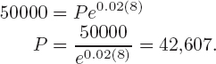
We can get the future value, B, from the present value, P, using B = Pert, so
Notice that since money was deposited at a rate of $1000 a year for 20 years, the total amount deposited was $20,000. The future value is $38,669, so the money has almost doubled because of the interest. |


Problems for Section 6.5
1. Draw a graph, with time in years on the horizontal axis, of what an income stream might look like for a company that sells sunscreen in the northeast United States.
2. Find the present and future values of an income stream of $12,000 a year for 20 years. The interest rate is 6%, compounded continuously.
3. Find the present and future values of an income stream of $2,000 per year for 15 years, assuming a 5% interest rate compounded continuously.
4. Assuming an interest rate of 3% compounded continuously,
(a) Find the future value in 10 years of a payment of $10,000 made today.
(b) Find the future value of an income stream of $1000 per year over 10 years.
(c) Which is larger, the future value from the lump sum in part (a) or from the income stream in part (b)? Explain why this makes sense financially.
5. Assuming an interest rate of 5% compounded continuously,
(a) Find the future value in 6 years of a payment of $12,000 made today.
(b) Find the future value of an income stream of $2000 per year over 6 years.
(c) Which is larger, the future value from the lump sum in part (a) or from the income stream in part (b)? Explain why this makes sense financially.
6. A person deposits money into an account, which pays 5% interest compounded continuously, at a rate of $1000 per year for 15 years. Calculate:
(a) The balance in the account at the end of the 15 years.
(b) The amount of money actually deposited into the account.
(c) The interest earned during the 15 years.
7. A person deposits money into an account, which pays 6% interest compounded continuously, at a rate of $1000 per year for 30 years. Calculate:
(a) The balance in the account at the end of the 30 years.
(b) The amount of money actually deposited into the account.
(c) The interest earned during the 30 years.
8. (a) Find the present and future value of an income stream of $6000 per year for a period of 10 years if the interest rate, compounded continuously, is 5%.
(b) How much of the future value is from the income stream? How much is from interest?
9. A small business expects an income stream of $5000 per year for a four-year period.
(a) Find the present value of the business if the annual interest rate, compounded continuously, is
(i) 3%
(ii) 10%
(b) In each case, find the value of the business at the end of the four-year period.
10. The Hershey Company is the largest US producer of chocolate. Between 2005 and 2008, Hershey generated net sales at a rate approximated by 4.8 + 0.1t billion dollars per year, where t is the time in years since January 1, 2005.4 Assume this rate continues through the year 2010 and that the interest rate is 2% per year compounded continuously.
(a) Find the value, on January 1, 2005, of Hershey's net sales during the five-year period from from January 1, 2005 to January 1, 2010.
(b) Find the value, on January 1, 2010, of Hershey's net sales during the same five-year period.
11. German TV and radio users pay an annual license fee of 200 euros. In 2008, the German poet Friedrich Schiller, who died in 1805, was sent reminders to pay his license fee.5 (The reminders were sent to an elementary school named after Schiller, despite a teacher pointing out that “the addressee is no longer in a position to listen to the radio or watch television”.) Assume the license fee had been charged at a continuous rate of 200 euros per year since 1805 and that the continous interest rate was 3% per year over this period. If Schiller were charged the license fee, with interest, since his death, how much would he have owed by 2008?
12. A recently installed machine earns the company revenue at a continuous rate of 60,000t + 45,000 dollars per year during the first six months of operation and at the continuous rate of 75,000 dollars per year after the first six months. The cost of the machine is $150,000, the interest rate is 7% per year, compounded continuously, and t is time in years since the machine was installed.
(a) Find the present value of the revenue earned by the machine during the first year of operation.
(b) Find how long it will take for the machine to pay for itself; that is, how long it will take for the present value of the revenue to equal the cost of the machine?
13. (a) A bank account earns 10% interest compounded continuously. At what constant, continuous rate must a parent deposit money into such an account in order to save $100,000 in 10 years for a child's college expenses?
(b) If the parent decides instead to deposit a lump sum now in order to attain the goal of $100,000 in 10 years, how much must be deposited now?
14. Your company needs $500,000 in two years' time for renovations and can earn 9% interest on investments.
(a) What is the present value of the renovations?
(b) If your company deposits money continuously at a constant rate throughout the two-year period, at what rate should the money be deposited so that you have the $500,000 when you need it?
15. A company is expected to earn $50,000 a year, at a continuous rate, for 8 years. You can invest the earnings at an interest rate of 7%, compounded continuously. You have the chance to buy the rights to the earnings of the company now for $350,000. Should you buy? Explain.
16. Sales of Version 6.0 of a computer software package start out high and decrease exponentially. At time t, in years, the sales are s(t) = 50,000e−t dollars per year. After two years, Version 7.0 of the software is released and replaces Version 6.0. You can invest earnings at an interest rate of 6%, compounded continuously. Calculate the total present value of sales of Version 6.0 over the two-year period.
17. Intel Corporation is a leading manufacturer of integrated circuits. In 2011, Intel generated profits at a continuous rate of 34.6 billion dollars per year based on a total revenue of 54 billion dollars.6 Assume the interest rate was 6% per year compounded continuously.
(a) What was the present value of Intel's profits over the 2011 one-year time period?
(b) What was the value at the end of the year of Intel's profits over the 2011 one-year time period?
18. Harley-Davidson Inc. manufactures motorcycles. During the years following 2003 (the company's 100th anniversary), the company's net revenue can be approximated7 by 4.6 + 0.4t billion dollars per year, where t is time in years since January 1, 2003. Assume this rate holds through January 1, 2014, and assume a continuous interest rate of 3.5% per year.
(a) What was the net revenue of the Harley-Davidson Company in 2003? What is the projected net revenue in 2013?
(b) What was the present value, on January 1, 2003, of Harley-Davidson's net revenue for the ten years from January 1, 2003 to January 1, 2013?
(c) What is the future value, on January 1, 2013, of net revenue for the preceding 10 years?
19. McDonald's Corporation licenses and operates a chain of 31,377 fast-food restaurants throughout the world. Between 2005 and 2008, McDonald's has been generating revenue at continuous rates between 17.9 and 22.8 billion dollars per year.8 Suppose that McDonald's rate of revenue stays within this range. Use an interest rate of 4.5% per year compounded continuously. Fill in the blanks:
(a) The present value of McDonald's revenue over a five-year time period is between __________ and__________billion dollars.
(b) The present value of McDonald's revenue over a twenty-five-year time period is between __________and__________billion dollars.
20. Your company is considering buying new production machinery. You want to know how long it will take for the machinery to pay for itself; that is, you want to find the length of time over which the present value of the profit generated by the new machinery equals the cost of the machinery. The new machinery costs $130,000 and earns profit at the continuous rate of $80,000 per year. Use an interest rate of 8.5% per year compounded continuously.
21. An oil company discovered an oil reserve of 100 million barrels. For time t > 0, in years, the company's extraction plan is a linear declining function of time as follows:
![]()
where q(t) is the rate of extraction of oil in millions of barrels per year at time t and b = 0.1 and a = 10.
(a) How long does it take to exhaust the entire reserve?
(b) The oil price is a constant $20 per barrel, the extraction cost per barrel is a constant $10, and the market interest rate is 10% per year, compounded continuously. What is the present value of the company's profit?
22. The value of good wine increases with age. Thus, if you are a wine dealer, you have the problem of deciding whether to sell your wine now, at a price of $P a bottle, or to sell it later at a higher price. Suppose you know that the amount a wine-drinker is willing to pay for a bottle of this wine t years from now is $P(1 + 20![]() ). Assuming continuous compounding and a prevailing interest rate of 5% per year, when is the best time to sell your wine?
). Assuming continuous compounding and a prevailing interest rate of 5% per year, when is the best time to sell your wine?
6.6 INTEGRATION BY SUBSTITUTION
In Chapter 3, we learned rules to differentiate any function obtained by combining constants, powers of x, sin x, cos x, ex, and ln x, using addition, multiplication, division, or composition of functions. Such functions are called elementary.
There is a great difference between looking for derivatives and looking for antiderivatives. Every elementary function has elementary derivatives, but many elementary functions do not have elementary antiderivatives. Some examples are ![]() and e−x2; these are ordinary functions that arise naturally.
and e−x2; these are ordinary functions that arise naturally.
In this section, we introduce integration by substitution which reverses the chain rule. According to the chain rule,

Thus, any function which is the result of differentiating with the chain rule is the product of two factors: the “derivative of the outside” and the “derivative of the inside.” If a function has this form, its antiderivative is f(g(x)) + C.
| Example 1 | Use the chain rule to find f′(x) and then write the corresponding antidifferentiation formula.
|
| Solution | (a) Using the chain rule, we see
(b) Using the chain rule, we see
(c) Using the chain rule, we see
|
In Example 1, the derivative of each inside function is 2x. Notice that the derivative of the inside function is a factor in the integrand in each antidifferentiation formula.
Finding an inside function whose derivative appears as a factor is key to the method of substitution. We formalize this method as follows:
To Make a Substitution in an Integral
Let w be the “inside function” and dw = ![]() . Then express the integrand in terms of w.
. Then express the integrand in terms of w.
| Example 2 | Make a substitution to find each of the following integrals:
|
| Solution | (a) We look for an inside function whose derivative appears as a factor. In this case, the inside function is x2, with derivative 2x. We let w = x2. Then dw = w′(x) dx = 2x dx. The original integrand can now be rewritten in terms of w:
By changing the variable to w, we simplified the integrand. The final step, after antidifferentiating, is to convert back to the original variable, x. (b) Here, the inside function is x2 + 1, with derivative 2x. We let w = x2 + 1. Then dw = w′(x) dx = 2x dx. Rewriting the original integral in terms of w, we have
Again, by changing the variable to w, we simplified the integrand. (c) The inside function is x2 + 4, so we let w = x2 + 4. Then dw = w′(x) dx = 2x dx. Substituting, we have
|
Notice that the derivative of the inside function must be present in the integral for this method to work. The method works, however, even when the derivative is missing a constant factor, as in the next two examples.
| Example 3 | Find |
| Solution | Here the inside function is t2 + 1, with derivative 2t. Since there is a factor of t in the integrand, we try w = t2 + 1. Then dw = w′(t) dt = 2t dt. Notice, however, that the original integrand has only t dt, not 2t dt. We therefore write
and then substitute:
|

Why didn't we put ![]() in the preceding example? Since the constant C is arbitrary, it does not really matter whether we add C or
in the preceding example? Since the constant C is arbitrary, it does not really matter whether we add C or ![]() . The convention is always to add C to whatever antiderivative we have calculated.
. The convention is always to add C to whatever antiderivative we have calculated.
| Example 4 | Find |
| Solution | The inside function is x4 + 5, with derivative 4x3. The integrand has a factor of x3, and since the only thing missing is a constant factor, we try
Then
giving
Then
|

Warning
We saw in the preceding examples that we can apply the substitution method when a constant factor is missing from the derivative of the inside function. However, we may not be able to use substitution if anything other than a constant factor is missing. For example, setting w = x4 + 5 to find
![]()
does us no good because x2 dx is not a constant multiple of dw = 4x3 dx. In order to use substitution, it helps if the integrand contains the derivative of the inside function, to within a constant factor.
| Example 5 | Find |
| Solution | Observing that the derivative of 1 + t3 is 3t2, we take w = 1 + t3, dw = 3t2 dt, so
Since the numerator is t2 dt, we might have tried w = t3. This substitution leads to the integral |

Using Substitution with Periodic Functions
The method of substitution can be used for integrals involving periodic functions.

| Example 7 | Find |
| Solution | We let w = cos θ since its derivative is − sin θ and there is a factor of sin θ in the integrand. This gives
so
Thus,
|
Definite Integrals by Substitution
The following example shows two ways of computing a definite integral by substitution.
| Example 8 | Compute  . . |
| Solution | To evaluate this definite integral using the Fundamental Theorem of Calculus, we first need to find an antiderivative of f(x) = xex2. The inside function is x2, so we let w = x2. Then dw = 2x dx, so
Now we find the definite integral:
There is another way to look at the same problem. After we established that
our next two steps were to replace w by x2, and then x by 2 and 0. We could have directly replaced the original limits of integration, x = 0 and x = 2, by the corresponding w limits. Since w = x2, the w limits are w = 02 = 0 (when x = 0) and w = 22 = 4 (when x = 2), so we get
As we would expect, both methods give the same answer. |


To Use Substitution to Find Definite Integrals
Either
- Compute the indefinite integral, expressing an antiderivative in terms of the original variable, and then evaluate the result at the original limits,
or
- Convert the original limits to new limits in terms of the new variable and do not convert the antiderivative back to the original variable.
Problems for Section 6.6
1. (a) Find the derivatives of sin(x2 + 1) and sin(x3 + 1).
(b) Use your answer to part (a) to find antiderivatives of:
(i) x cos(x2 + 1)
(ii) x2 cos(x3 + 1)
(c) Find the general antiderivatives of:
(i) x sin(x2 + 1)
(ii) x2 sin(x3 + 1)
In Problems 2–5 explain how you can tell if substitution can be used to find an antiderivative.
2. ![]()
3. ![]()
4. ![]()
5. ![]()
Find the integrals in Problems 6–47. Check your answers by differentiation.
6. ![]() 2x(x2 + 1)5 dx
2x(x2 + 1)5 dx
7. ![]()
8. ![]() (5x −7)10 dx
(5x −7)10 dx
9. ![]()
10. ![]() 2qeq2+1dq
2qeq2+1dq
11. ![]() 5e5t+2dt
5e5t+2dt
12. ![]() xe −x2 dx
xe −x2 dx
13. ![]() 100e−0.2t dt
100e−0.2t dt
14. ![]() t2 (t3 −3)10 dt
t2 (t3 −3)10 dt
15. ![]() x sin(x2)dx
x sin(x2)dx
16. ![]() x(x2 −4)7/2 dx
x(x2 −4)7/2 dx
17. ![]() x(x2 + 3)2 dx
x(x2 + 3)2 dx
18. ![]()
19. ![]()
20. ![]() 12x2 cos(x3)dx
12x2 cos(x3)dx
21. ![]() (2t −7)73 dt
(2t −7)73 dt
22. ![]() (x2 + 3)2 dx
(x2 + 3)2 dx
23. ![]() y2 (1 + y)2 dy
y2 (1 + y)2 dy
24. ![]() sin θ(cos θ +5)7 dθ
sin θ(cos θ +5)7 dθ
25. ![]() sin6 θ cos θ dθ
sin6 θ cos θ dθ
26. ![]()
27. ![]() sin(3 −t)dt
sin(3 −t)dt
28. ![]()
29. ![]()
30. ![]() sin3 α cos α dα
sin3 α cos α dα
31. ![]() x sin(4x2)dx
x sin(4x2)dx
32. ![]() sin2 x cos xdx
sin2 x cos xdx
33. ![]() e3x−4 dx
e3x−4 dx
34. ![]()
35. ![]()
36. ![]()
37. ![]()
38. ![]()
39. ![]()
40. ![]()
41. ![]()
42. 
43. ![]()
44. ![]()
45. ![]()
46. ![]() sin6 (5θ) cos(5θ) dθ
sin6 (5θ) cos(5θ) dθ
47. 
48. If appropriate, evaluate the following integrals by substitution. If substitution is not appropriate, say so, and do not evaluate.
(a) ![]() x sin(x2)dx
x sin(x2)dx
(b) ![]() x2 sin x dx
x2 sin x dx
(c) ![]()
(d) ![]()
(e) ![]()
(f) ![]()
49. Use substitution to express each of the following integrals as a multiple of ![]() for some a and b. Then evaluate the integrals.
for some a and b. Then evaluate the integrals.
(a) 
(b) 
Use integration by substitution and the Fundamental Theorem to evaluate the definite integrals in Problems 50–59.
50. 
51. 
52. 
53. ![]()
54. 
55. 

57. 
58. 
59. 
In Problems 60–61, find the exact area.
60. Under f(x) = xex2 between x = 0 and x = 2.
61. Under f(x)= 1/(x + 1) between x = 0 and x = 2.
62. Find the exact average value of f(x) = 1/(x + 1) on the interval x = 0 to x = 2. Sketch a graph showing the function and the average value.
63. Suppose ![]() . Calculate the following:
. Calculate the following:
(a) 
(b) 
64. (a) Find ![]() in two ways:
in two ways:
(i) By multiplying out
(ii) By substituting w = x + 5
(b) Are the results the same? Explain.
65. Find ![]() using two methods:
using two methods:
(a) Do the multiplication first, and then antidifferentiate.
(b) Use the substitution w = x2 + 1.
(c) Explain how the expressions from parts (a) and (b) are different. Are they both correct?
66. (a) Find ![]() sin θ cos θ dθ.
sin θ cos θ dθ.
(b) You probably solved part (a) by making the substitution w = sin θ or w = cos θ. (If not, go back and do it that way.) Now find ![]() sin θ cos θ dθ by making the other substitution.
sin θ cos θ dθ by making the other substitution.
(c) There is yet another way of finding this integral which involves the trigonometric identities
![]()
Find ![]() sin θ cos θ dθ using one of these identities and then the substitution w = 2θ.
sin θ cos θ dθ using one of these identities and then the substitution w = 2θ.
(d) You should now have three different expressions for the indefinite integral ![]() sin θ cos θ dθ. Are they really different? Are they all correct? Explain.
sin θ cos θ dθ. Are they really different? Are they all correct? Explain.
6.7 INTEGRATION BY PARTS
Now we introduce integration by parts, which is a technique for finding integrals based on the product rule. We begin with the product rule:
![]()
where u and v are functions of x with derivatives u′ and v′, respectively. We rewrite this as:
![]()
and then integrate both sides:
![]()
Since an antiderivative of ![]() is just uv, we get the following formula:
is just uv, we get the following formula:
Integration by Parts
![]()
This technique is useful when the integrand can be viewed as a product and when the integral on the right-hand side is simpler than that on the left.
| Example 1 | Use integration by parts to find |
| Solution | We let xex = (x) · (ex) = uv′, and choose u = x and v′ = ex. Thus, u′ = 1 and v = ex, so
|
Let's look again at Example 1. Notice what would have happened if we took v = ex + C1. Then

as before. Thus, it is not necessary to include an arbitrary constant in the antiderivative for v; any antiderivative will do.
What would have happened if we had picked u and v′ the other way around in Example 1? If u = ex and v′ = x, then u′ = ex and v = x2/2. The formula for integration by parts then gives
![]()
which is true but not helpful, since the new integral on the right seems harder than the original one on the left. To use this method, we must choose u and v′ to make the integral on the right no harder to find than the integral on the left.
How to Choose u and v′
- Whatever you let v′ be, you need to be able to find v.
- It helps if u′v is simpler (or at least no more complicated) than uv′.
| Example 2 | Find |
| Solution | We let xe3x = (x) · (e3x) = uv′, and choose u = x and v′ = e3x. Thus, u′ = 1 and
|

There are some examples which don't look like good candidates for integration by parts because they don't appear to involve products, but for which the method works well. Such examples often involve ln x. Here is one:
| Example 3 | Find  . . |
| Solution | The integrand does not look like a product unless we write ln x = (1)(ln x). We might say u = 1 so u′ = 0, which certainly makes things simpler. But if v′ = ln x, what is v? If we knew, we would not need integration by parts. Let's try the other way: if u = ln x, u′ = 1/x and if v′ = 1, v = x, so
|

Notice that when doing a definite integral by parts, we must remember to put the limits of integration (here 2 and 3) on the uv term (in this case x ln x) as well as on the integral ![]() u′v dx.
u′v dx.
| Example 4 | Find |
| Solution | We can write x6 ln x as uv′ where u = ln x and v′ = x6. Then v =
|

In Example 4 we did not choose v′ = ln x, because it is not immediately clear what v would be. In fact, we used integration by parts in Example 3 to find the antiderivative of ln x. Also, using u = ln x, as we have done, gives u′v = x6/7, which is simpler to integrate than uv′ = x6 ln x. This example shows that u does not have to be the first factor in the integrand (here x6).
Problems for Section 6.7
Find the integrals in Problems 1–14.
1. ![]() te5t dt
te5t dt
2. ![]() pe−0.1p dp
pe−0.1p dp
3. ![]() y ln y dy
y ln y dy
4. ![]() (z + 1)e2z dz
(z + 1)e2z dz
5. ![]() q5 ln 5q dq
q5 ln 5q dq
6. ![]()
7. ![]() x3 ln x dx
x3 ln x dx
8. ![]()
9. ![]()
10. ![]()
11. ![]()
12. ![]()
13. ![]() t sin t dt
t sin t dt
14. ![]() (θ + 1) sin(θ + 1) dθ
(θ + 1) sin(θ + 1) dθ
15. Find ![]() ln x dx numerically. Find
ln x dx numerically. Find ![]() ln x dx using antiderivatives. Check that your answers agree.
ln x dx using antiderivatives. Check that your answers agree.
Evaluate the integrals in Problems 16–20 both exactly [e.g. ln(3π)] and numerically [e.g. ln(3π) ≈ 2.243].
16. ![]()
17. ![]()
18. ![]()
19. ![]()
20. ![]()
In Problems 21–22, use integration by parts twice to evaluate the integral.
21. ![]() (ln t2) dt
(ln t2) dt
22. ![]() t2e5t dt
t2e5t dt
23. For each of the following integrals, indicate whether integration by substitution or integration by parts is more appropriate. Do not evaluate the integrals.
(a) ![]()
(b) ![]()
(c) ![]()
(d) ![]()
(e) ![]()
(f) ![]()
In Problems 24–25, find the exact area.
24. Under y = te−t for 0 ≤ t ≤ 2.
25. Between y = ln x and y = ln(x2) for 1 ≤ x ≤ 2.
26. The concentration, C, in ng/ml, of a drug in the blood as a function of the time, t, in hours since the drug was administered is given by C = 15te−0.2t. The area under the concentration curve is a measure of the overall effect of the drug on the body, called the bioavailability. Find the bioavailability of the drug between t = 0 and t = 3.
27. During a surge in the demand for electricity, the rate, r, at which energy is used can be approximated by
![]()
where t is the time in hours and a is a positive constant.
(a) Find the total energy, E, used in the first T hours. Give your answer as a function of a.
(b) What happens to E as T → ∞?
CHAPTER SUMMARY
- Computing antiderivatives
Powers and polynomials, ekx, sin(kx), cos(kx)
- Integration by substitution
- Integration by parts
- Using antiderivatives to compute definite integrals analytically: Fundamental Theorem of Calculus
- Using definite integrals to analyze antiderivatives numerically and graphically
- Improper integrals
- Consumer and producer surplus
Wage and price controls
- Present and future value
REVIEW PROBLEMS FOR CHAPTER SIX
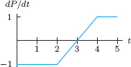
1. Use Figure 6.39 and the fact that P = 2 when t = 0 to find values of P when t = 1, 2, 3, 4 and 5.
In Problems 2–3, sketch two functions F such that F′ = f. In one case let F(0) = 0 and in the other, let F(0) = 1.
2.

3.

4. Figure 6.40 shows the derivative F′ (x). If F(0) = 5, find the value of F(1), F(3), and F(4).

Problems 5–6 show the derivative f′ of f.
(a) Where is f increasing and where is f decreasing? What are the x-coordinates of the local maxima and minima of f?
(b) Sketch a possible graph for f. (You don't need a scale on the vertical axis.)
5.

6.

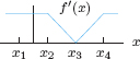
Problems 7–8 give a graph of f′ (x). Graph f(x). Mark the points x1 , . . . , x4 on your graph and label local maxima, local minima and points of inflection.
7.
8.

In Problems 9–18, find an antiderivative
9. h(t)= 3t2 + 7t + 1
10. f(t)= 2t2 + 3t3 + 4t4
11. f(x)= 6x2 −8x + 3
12. ![]()
13. f(x)= 3x2 + 5
14. ![]()
15. ![]()
16. g(t) = sin t
17. f(x) = (2x + 1)3
18. g(x) = (x + 1)3
In Problems 19–29, find the indefinite integrals.
19. ![]()
20. ![]()
21. ![]()
22. ![]()
23. ![]()
24. ![]()
25. ![]()
26. ![]()
27. ![]()
28. ![]()
29. ![]()
Find the definite integrals in Problems 30–35 using the Fundamental Theorem.
30. ![]()
31. ![]()
32. ![]()
33. ![]()
34. ![]()
35. ![]()
36. Use the Fundamental Theorem to find the area under f(x) = x2 between x = 1 and x = 4.
37. Write the definite integral for the area under the graph of f(x) = 6x2 + 1 between x = 0 and x = 2. Use the Fundamental Theorem of Calculus to evaluate it.
38. Use the Fundamental Theorem to find the average value of f(x) = x2 + 1 on the interval x = 0 to x = 10. Illustrate your answer on a graph of f(x).
39. Use the Fundamental Theorem to determine the value of b if the area under the graph of f(x) = 8x between x = 1 and x = b is equal to 192. Assume b > 1.
40. Find the exact area below the curve y = x3 (1 − x) and above the x-axis.
41. Find the exact area enclosed by the curve y = x2 (1 − x)2 and the x-axis.
42. (a) Sketch the area represented by the improper integral ![]() .
.
(b) Calculate ![]() for b = 5, 10, 20.
for b = 5, 10, 20.
(c) The improper integral in part (a) converges. Use your answers to part (b) to estimate its value.
43. Consider the improper integral
![]()
(a) Use a calculator or computer to find ![]() for b = 100, 1000, 10,000. What do you notice?
for b = 100, 1000, 10,000. What do you notice?
(b) Find ![]() using the Fundamental Theorem of Calculus. Your answer will contain b.
using the Fundamental Theorem of Calculus. Your answer will contain b.
(c) Now take the limit as b → ∞. What does this tell you about the improper integral?
44. (a) Find ![]() = 10, 50, 100, 200.
= 10, 50, 100, 200.
(b) Assuming that it converges, estimate the value of ![]() .
.
45. A car moves with velocity, v, at time t in hours given by
![]()
(a) Does the car ever stop?
(b) Write an integral representing the total distance traveled for t ≥ 0.
(c) Do you think the car goes a finite distance for t ≥ 0? If so, estimate that distance.
46. With t in years since 2000, the population, P, of the world in billions can be modeled by P = 6.1e0.012t.
(a) What does this model predict for the world population in 2010? In 2020?
(b) Use the Fundamental Theorem to predict the average population of the world between 2000 and 2010.
47. For a product, the supply curve is p = 5 + 0.02q and the demand curve is p = 30e−0.003q, where p is the price and q is the quantity sold at that price. Find:
(a) The equilibrium price and quantity
(b) The consumer and producer surplus
48. Show graphically that the maximum total gains from trade occurs at the equilibrium price. Do this by showing that if outside forces keep the price artificially high or low, the total gains from trade (consumer surplus + producer surplus) are lower than at the equilibrium price.
49. In May 1991, Car and Driver described a Jaguar that sold for $980,000. At that price only 50 have been sold. It is estimated that 350 could have been sold if the price had been $560,000. Assuming that the demand curve is a straight line, and that $560,000 and 350 are the equilibrium price and quantity, find the consumer surplus at the equilibrium price.
50. The demand curve for a product has equation p = 20e−0.002q and the supply curve has equation p = 0.02q + 1 for 0 ≤ q ≤ 1000, where q is quantity and p is price in $/unit.
(a) Which is higher, the price at which 300 units are supplied or the price at which 300 units are demanded? Find both prices.
(b) Sketch the supply and demand curves. Find the equilibrium price and quantity.
(c) Using the equilibrium price and quantity, calculate and interpret the consumer and producer surplus.
51. Calculate the present value of a continuous revenue stream of $1000 per year for 5 years at an interest rate of 9% per year compounded continuously.
52. At what constant, continuous rate must money be deposited into an account if the account is to contain $20,000 in 5 years? The account earns 6% interest compounded continuously.
53. A bond is guaranteed to pay 100 + 10t dollars per year for 10 years, where t is in years from the present. Find the present value of this income stream, given an interest rate of 5%, compounded continuously.
54. Determine the constant income stream that needs to be invested over a period of 10 years at an interest rate of 5% per year compounded continuously to provide a present value of $5000.
55. In 1980, before the unification of Germany in 1990 and the introduction of the Euro, West Germany made a loan of 20 billion Deutsche Marks to the Soviet Union, to be used for the construction of a natural gas pipeline connecting Siberia to Western Russia, and continuing to West Germany (Urengoi-Uschgorod-Berlin). Assume that the deal was as follows: In 1985, upon completion of the pipeline, the Soviet Union would deliver natural gas to West Germany, at a constant rate, for all future times. Assuming a constant price of natural gas of 0.10 Deutsche Mark per cubic meter, and assuming West Germany expects 10% annual interest on its investment (compounded continuously), at what rate does the Soviet Union have to deliver the gas, in billions of cubic meters per year? Keep in mind that delivery of gas could not begin until the pipeline was completed. Thus, West Germany received no return on its investment until after five years had passed. (Note: A more complex deal of this type was actually made between the two countries.)
In Problems 56–58, find an antiderivative F(x) with F′(x) = f(x) and F(0) = 0. Is there only one possible solution?
56. f(x) = 2x
57. f(x) = −7x
58. ![]()
In Problems 59–68, integrate by substitution.
59. ![]()
60. ![]()
61. ![]()
62. ![]()
63. ![]()
64. ![]()
65. ![]()
66. ![]()
67. ![]()
68. ![]()
69. Estimate ![]() if f(x) = x2 and g has the values in the following table.
if f(x) = x2 and g has the values in the following table.
![]()
70. Derive the formula (called a reduction formula):
![]()
In Problems 71–73 use integration by parts to evaluate the in-definite integral. Check your answer by differentiating.
71. ![]()
72. ![]()
73. ![]()
STRENGTHEN YOUR UNDERSTANDING
In Problems 1–70, indicate whether the statement is true or false.
1. If a function f is positive on an interval, then its antiderivatives are all increasing on that interval.
2. If a function f is increasing on an interval, then its antiderivatives are all concave up on that interval.
3. For any function F with continuous derivative, F(5) = ![]()
4. For any function F with continuous derivative, F(3) = ![]()
5. If f′ is in Figure 6.41, then f (4) > f(3).

6. If f′ is in Figure 6.41, then f(2) > f (1).
7. If f′ is in Figure 6.41, then f(3) > f (2).
8. If f′ is in Figure 6.41, then f (5) > f (6).
9. If f′ is in Figure 6.41, then f (1) > f (0).
10. If f′ is in Figure 6.41, then f (1) ≈ f(3).
11. ![]() is an antiderivative of f(t) = t2.
is an antiderivative of f(t) = t2.
12. ![]() is an antiderivative of f(x) = x−2.
is an antiderivative of f(x) = x−2.
13. ![]() is an antiderivative of f(x) = e3x.
is an antiderivative of f(x) = e3x.
14. ![]()
15. ![]()
16. ![]()
17. ![]()
19. ![]()
20. If F(x) and G(x) are both antiderivatives of h(x), then F(x) − G(x) is a constant.
21. ![]() .
.
22. ![]()
23. ![]() .
.
24. ![]() .
.
25. ![]() .
.
26. ![]() .
.
27. The substitution w = x2 converts ![]() into
into ![]()
28. The substitution w = ln x converts ![]() into
into ![]()
29. If f(x) is any function then ![]() .
.
30. The integral ![]() is positive for any k ≠ 0.
is positive for any k ≠ 0.
31. The supply curve shows the quantity of an item that a producer supplies at different prices.
32. The demand curve shows the quantity of an item that consumers will purchase at various prices.
33. The equilibrium price p* is where the demand curve crosses the q-axis.
34. Consumer surplus is the total amount gained by consumers by purchasing items at prices higher than they are willing to pay.
35. The units of consumer surplus are the same as the units of producer surplus.
36. The units of producer surplus are price times quantity.
37. Total gains from trade is the difference between consumer and producer surplus.
38. The area under the demand curve from 0 to the equilibrium quantity q* is the amount consumers spend at the equilibrium price p*.
39. Consumer surplus at price p* is the area between the demand curve and the horizontal line at p*.
40. Producer surplus at price p* is the area between the demand curve and the horizontal line at p*.
41. Assuming a positive interest rate, the present value of an income stream is always less than its future value.
42. The future value of an income stream of $1000 per year for 5 years is more than $5000 if the interest rate is 2%.
43. The present value of an income stream of $1000 per year for 5 years is more than $5000 if the interest rate is 2%.
44. A single payment at the beginning of the year of $1000 has the same future value as an income stream of $1000 per year if we assume a continuous interest rate of 3% for one year for both.
45. If S(t) is an income stream, then S(t) has units of dollars.
46. With a continuous interest rate of r, the future value of a payment of $3000 today in 5 years is 3000e−5r.
47. With a continuous interest rate of r, we would have to deposit 3000e−5r today to grow to $3000 in 5 years.
48. If an income stream of 2000 dollars per year grows to $11,361 in five years, then the amount of interest earned over the five-year period is $1361.
49. The present value of an income stream of 2000 dollars per year that starts now and pays out over 6 years with a continuous interest rate of 2% is ![]() .
.
50. The future value of an income stream of 2000 dollars per year that starts now and accumulates over 9 years with a positive interest rate is greater than $18,000.
51. The substitution w = q3 + 3q2 − q converts the integral ![]() into
into ![]() .
.
52. The substitution w = ln x converts the integral ![]()
53. The substitution w = x2 converts the integral ![]() into
into ![]()
54. The substitution w = x2 converts the integral ![]() into
into ![]()
55. The substitution w = 1 − s converts the integral ![]() into
into ![]() .
.
56. The substitution w = t2 + 1 converts the integral ![]() into
into ![]()
57. The substitution w = ex + e−x converts the integral ![]() into
into ![]()
58. The substitution w = q3 converts the integral ![]() q2(q3 + 5)10 dq into
q2(q3 + 5)10 dq into ![]()
59. The substitution w = sin α converts the integral ![]() sin3 α cos α dα into
sin3 α cos α dα into ![]() w3 dw.
w3 dw.
60. The substitution w = cos x converts the integral ![]()
61. Setting u = x3/3 and dv = ex dx is a reasonable assignment of the parts for the integral ![]() x2exdx.
x2exdx.
62. Setting u = x and dv = ![]() is a reasonable assignment of the parts for the integral
is a reasonable assignment of the parts for the integral ![]()
63. If u = x2 and dv = e3x dx in integration by parts, then du = 2x dx and v = 3e3x.
64. If u = x2 and dv = ln x dx in integration by parts, then du = 2x dx and v = 1/x.
65. Integration by parts is an appropriate method to use in evaluating ![]()
66. Integration by parts is an appropriate method to use in evaluating ![]() .
.
67. Integration by parts is an appropriate method to use in evaluating ![]()
68. Integration by parts is an appropriate method to use in evaluating ![]()
69. Integration by parts is an appropriate method to use in evaluating ![]() .
.
70. Integration by parts is an appropriate method to use in evaluating ![]() .
.
PROJECTS FOR CHAPTER SIX
1. Quabbin Reservoir The Quabbin Reservoir in the western part of Massachusetts provides most of Boston's water. The graph in Figure 6.42 represents the flow of water in and out of the Quabbin Reservoir throughout 2007.
(a) Sketch a graph of the quantity of water in the reservoir, as a function of time.
(b) When, in the course of 2007, was the quantity of water in the reservoir largest? Smallest? Mark and label these points on the graph you drew in part (a).
(c) When was the quantity of water increasing most rapidly? Decreasing most rapidly? Mark and label these times on both graphs.
(d) By July 2008 the quantity of water in the reservoir was about the same as in January 2007. Draw plausible graphs for the flow into and the flow out of the reservoir for the first half of 2008.
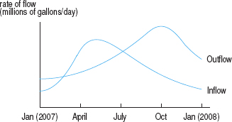
2. Distribution of Resources
Whether a resource is distributed evenly among members of a population is often an important political or economic question. How can we measure this? How can we decide if the distribution of wealth in this country is becoming more or less equitable over time? How can we measure which country has the most equitable income distribution? This problem describes a way of making such measurements. Suppose the resource is distributed evenly. Then any 20% of the population will have 20% of the resource. Similarly, any 30% will have 30% of the resource and so on. If, however, the resource is not distributed evenly, the poorest p% of the population (in terms of this resource) will not have p% of the goods. Suppose F(x) represents the fraction of the resource owned by the poorest fraction x of the population. Thus F(0.4) = 0.1 means that the poorest 40% of the population owns 10% of the resource.
(a) What would F be if the resource were distributed evenly?
(b) What must be true of any such F? What must F (0) and F (1) equal? Is F increasing or decreasing? Is the graph of F concave up or concave down?
(c) Gini's index of inequality, G, is one way to measure how evenly the resource is distributed. It is defined by
![]()
Show graphically what G represents.
(d) Graphical representations of Gini's index for two countries are given in Figures 6.43 and 6.44. Which country has the more equitable distribution of wealth? Discuss the distribution of wealth in each of the two countries.


(e) What is the maximum possible value of Gini's index of inequality, G? What is the minimum possible value? Sketch graphs in each case. What is the distribution of resources in each case?
3. Yield from an Apple Orchard
Figure 6.45 is a graph of the annual yield, y(t), in bushels per year, from an orchard t years after planting. The trees take about 10 years to get established, but for the next 20 years they give a substantial yield. After about 30 years, however, age and disease start to take their toll, and the annual yield falls off.9
(a) Represent on a sketch of Figure 6.45 the total yield, F(M), up to M years, with 0 ≤ M ≤ 60. Write an expression for F(M) in terms of y(t).
(b) Sketch a graph of F (M) against M for 0 ≤ M ≤ 60.
(c) Write an expression for the average annual yield, a(M), up to M years.
(d) When should the orchard be cut down and replanted? Assume that we want to maximize average revenue per year, and that fruit prices remain constant, so that this is achieved by maximizing average annual yield. Use the graph of y(t) to estimate the time at which the average annual yield is a maximum. Explain your answer geometrically and symbolically.

FOCUS ON PRACTICE
For Problems 1–47, evaluate the integrals. Assume a, b, A, B, P0, h, and k are constants.
1. ![]()
2. ![]()
3. ![]()
4. ![]()
5. ![]()
6. ![]()
7. ![]()
8. ![]()
9. ![]()
10. ![]()
11. ![]()
12. ![]()
13. ![]()
14. ![]()
15. ![]()
16. ![]()
17. ![]()
18. ![]()
19. ![]()
20. ![]()
21. ![]()
22. ![]()
23. ![]()
24. ![]()
25. ![]()
26. ![]()
27. ![]()
28. ![]()
29. ![]()
30. ![]()
31. ![]()
32. ![]()
33. ![]()
34. ![]()
35. ![]()
36. ![]()
37. ![]()
38. ![]()
39. ![]()
40. ![]()
41. ![]()
42. ![]()
43. ![]()
44. ![]()
45. ![]()
46. ![]()
47. ![]()
1Based on: Reich et al., Response of Soybean to Low Concentrations of Ozone: I. Reductions in Leaf and Whole Plant Net Photosynthesis and Leaf Chlorophyll Content, Journal of Environmental Quality, 1986, 15(1).
2Based on data from www.esrl.noaa.gov/gmd/ccgg. Accesed March 13, 2013
3Note that here p is written as a function of q.
42008 Annual Report, accessed at www.thehersheycompany.com, accessed March 13, 2013.
5http://news.bbc.co.uk/2/hi/europe/7648021.stm, accessed January 2013.
6http://www.intc.com/financials.cfm, accessed May 2012.
72007 Harley-Davidson Annual Report, accessed from www.harley-davidson.com.
8McDonald's Annual Report 2007, www.mcdonalds.com, accessed March 13, 2013.
9From Peter D. Taylor, Calculus: The Analysis of Functions (Toronto: Wall & Emerson, Inc., 1992).