

Chapter Eight
FUNCTIONS OF SEVERAL VARIABLES
Contents
8.1 Understanding Functions of Two Variables
Strategy to Investigate Functions of Two Variables: Vary One Variable at a Time
Concentration of a Drug in the Blood
Cobb-Douglas Production Functions
Finding Contours Algebraically
Rate of Change of Airline Revenue
Estimating Partial Derivatives from a Table
Using Partial Derivatives to Estimate Values of the Function
Estimating Partial Derivatives from Contours
Using Units to Interpret Partial Derivatives
8.4 Computing Partial Derivatives Algebraically
Second-Order Partial Derivatives
The Mixed Partial Derivatives Are Equal
8.5 Critical Points and Optimization
Finding Local Maxima/Minima Analytically
How Do We Find Critical Points?
Is a Critical Point a Local Maximum or a Local Minimum?
Graphical Approach: Maximizing Production Subject to a Budget Constraint
8.1 UNDERSTANDING FUNCTIONS OF TWO VARIABLES
In business, science, and politics, outcomes are rarely determined by a single variable. For example, consider an airline's ticket pricing. To avoid flying planes with many empty seats, it sells some tickets at full price and some at a discount. For a particular route, the airline's revenue, R, earned in a given time period is determined by the number of full-price tickets, x, and the number of discount tickets, y, sold. We say that R is a function of x and y, and we write
![]()
This is just like the function notation of one-variable calculus. The variable R is the dependent variable and the variables x and y are the independent variables. The letter f stands for the function or rule that gives the value, or output, of R corresponding to given values of x and y. The collection of all possible inputs, (x, y), is called the domain of f. We say a function is an increasing (decreasing) function of one of its variables if it increases (decreases) as that variable increases while the other independent variables are held constant.
A function of two variables can be represented numerically by a table of values, algebraically by a formula, or pictorially by a contour diagram. In this section we give numerical and algebraic examples; contour diagrams are introduced in Section 8.2.
Functions Given Numerically
The revenue, R (in dollars), from a particular airline route is shown in Table 8.1 as a function of the number of full-price tickets and the number of discount tickets sold.
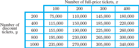
Values of x are shown across the top, values of y are down the left side, and the corresponding values of f(x, y) are in the table. For example, to find the value of f(300, 600), we look in the column corresponding to x = 300 at the row y = 600, where we find the number 225,000. Thus,
![]()
This means that the revenue from 300 full-price tickets and 600 discount tickets is $225,000. We see in Table 8.1 that f is an increasing function of x and an increasing function of y.
Notice how this differs from the table of values of a one-variable function, where one row or one column is enough to list the values of the function. Here many rows and columns are needed because the function has an output for every pair of values of the independent variables.
Functions Given Algebraically
The function given in Table 8.1 can be represented by a formula. Looking across the rows, we see that each additional 100 full-price tickets sold raises the revenue by $35,000, so each full-price ticket must cost $350. Similarly, looking down a column shows that an additional 200 discount tickets sold increases the revenue by $40,000, so each discount ticket must cost $200. Thus, the revenue function is given by the formula
![]()
| Example 2 | A car rental company charges $40 a day and 15 cents a mile for its cars.
(a) Write a formula for the cost, C, of renting a car as a function of the number of days, d, and the number of miles driven, m. (b) If C = f(d, m), find f(5,300) and interpret it. |
| Solution | (a) The total cost in dollars of renting a car is 40 times the numbers of days plus 0.15 times the number of miles, so
(b) We have
We see that f(5, 300) = 245. This tells us that if we rent a car for 5 days and drive it 300 miles, it costs us $245. |

Strategy to Investigate Functions of Two Variables: Vary One Variable at a Time
We can learn a great deal about a function of two variables by letting one variable vary while holding the other fixed. This gives a function of one variable, called a cross-section of the original function.
Concentration of a Drug in the Blood
When a drug is injected into muscle tissue, it diffuses into the bloodstream. The concentration of the drug in the blood increases until it reaches a maximum, and then decreases. The concentration, C (in mg per liter), of the drug in the blood is a function of two variables: x, the amount (in mg) of the drug given in the injection, and t, the time (in hours) since the injection was administered. We are told that
![]()
| Example 3 | In terms of the drug concentration in the blood, explain the significance of the cross-sections:
(a) f(4, t) (b) f(x, 1) |
| Solution | (a) Holding x fixed at 4 means that we are considering an injection of 4 mg of the drug; letting t vary means we are watching the effect of this dose as time passes. Thus the function f(4, t) describes the concentration of the drug in the blood resulting from a 4-mg injection as a function of time. Figure 8.1 shows the graph of f(4, t) = te−t. Notice that the concentration in the blood from this dose is at a maximum at 1 hour after injection, and that the concentration in the blood eventually approaches zero.
Figure 8.1: The function f(4, t) shows the concentration in the blood resulting from a 4-mg injection
Figure 8.2: The function f(x, 1) shows the concentration in the blood 1 hour after the injection (b) Holding t fixed at 1 means that we are focusing on the blood 1 hour after the injection; letting x vary means we are considering the effect of different doses at that instant. Thus, the function f(x, 1) gives the concentration of the drug in the blood 1 hour after injection as a function of the amount injected. Figure 8.2 shows the graph of f(x, 1) = e−(5−x) = ex−5. Notice that f(x, 1) is an increasing function of x. This makes sense: If we administer more of the drug, the concentration in the bloodstream is higher. |


| Example 4 | Continue with C = f(x, t) = te−t(5−x). Graph the cross-sections of f(a, t) for a = 1, 2, 3, and 4 on the same axes. Describe how the graph changes for larger values of a and explain what this means in terms of drug concentration in the blood. |
| Solution | The one-variable function f(a, t) represents the effect of an injection of a mg at time t. Figure 8.3 shows the graphs of the four functions f(1, t) = te−4t, f(2, t) = te−3t, f(3, t) = te−2t, and f(4, t) = te−t corresponding to injections of 1, 2, 3, and 4 mg of the drug. The general shape of the graph is the same in every case: The concentration in the blood is zero at the time of injection t = 0, then increases to a maximum value, and then decreases toward zero again. We see that if a larger dose of the drug is administered, the peak of the graph is later and higher. This makes sense, since a larger dose will take longer to diffuse fully into the bloodstream and will produce a higher concentration when it does.
Figure 8.3: Concentration C = f(a, t) of the drug resulting from an a-mg injection |

Problems for Section 8.1
Problems 1–2 concern the cost, C, of renting a car from a company which charges $40 a day and 15 cents a mile, so C = f(d, m) = 40d + 0.15m, where d is the number of days, and m is the number of miles.
1. Make a table of values for C, using d = 1, 2, 3, 4 and m = 100, 200, 300, 400. You should have 16 values in your table.
2. (a) Find f(3,200) and interpret it.
(b) Explain the significance of f(3, m) in terms of rental car costs. Graph this function, with C as a function of m.
(c) Explain the significance of f(d, 100) in terms of rental car costs. Graph this function, with C as a function of d.
3. The number, n, of new cars sold in a year is a function of the price of new cars, c, and the average price of gas, g.
(a) If c is held constant, is n an increasing or decreasing function of g? Why?
(b) If g is held constant, is n an increasing or decreasing function of c? Why?
Problems 4–8 refer to Table 8.2, which shows1 the weekly beef consumption, C, (in lbs) of an average household as a function of p, the price of beef (in $/lb) and I, annual household income (in $1000s).
Table 8.2 Quantity of beef bought (lbs/household/week)

4. Give tables for beef consumption as a function of p, with I fixed at I = 20 and I = 100. Give tables for beef consumption as a function of I, with p fixed at p = 3.00 and p = 4.00. Comment on what you see in the tables.
5. How does beef consumption vary as a function of household income if the price of beef is held constant?
6. Make a table showing the amount of money, M, that the average household spends on beef (in dollars per household per week) as a function of the price of beef and household income.
7. Make a table of the proportion, P, of household income spent on beef per week as a function of price and income. (Note that P is the fraction of income spent on beef.)
8. Express P, the proportion of household income spent on beef per week, in terms of the original function f(I, p) which gave consumption as a function of p and I.
9. The total sales of a product, S, can be expressed as a function of the price p charged for the product and the amount, a, spent on advertising, so S = f(p, a). Do you expect f to be an increasing or decreasing function of p? Do you expect f to be an increasing or decreasing function of a? Why?
10. Graph the bank-account function f in Example 1 on page 354, holding B fixed at B = 10, 20, 30 and letting t vary. Then graph f, holding t fixed at t = 0, 5, 10 and letting B vary. Explain what you see.
11. The heat index is a temperature which tells you how hot it feels as a result of the combination of temperature and humidity. See Table 8.3. Heat exhaustion is likely to occur when the heat index reaches 105° F.
(a) If the temperature is 80°F and the humidity is 50%, how hot does it feel?
(b) At what humidity does 90°F feel like 90°F?
(c) Make a table showing the approximate temperature at which heat exhaustion becomes a danger, as a function of humidity.
(d) Explain why the heat index is sometimes above the actual temperature and sometimes below it.
Table 8.3 Heat index (°F) as a function of humidity (H%) and temperature (T°F)

12. Using Table 8.3, graph heat index as a function of humidity with temperature fixed at 70°F and at 100°F. Explain the features of each graph and the difference between them in common-sense terms.
13. The monthly payments, P dollars, on a mortgage in which A dollars were borrowed at an annual interest rate of r% for t years is given by P = f(A, r, t). Is f an increasing or decreasing function of A? Of r? Of t?
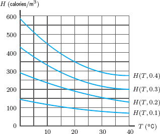
14. An airport can be cleared of fog by heating the air. The amount of heat required, H(T, w) (in calories per cubic meter of fog), depends on the temperature of the air, T (in °C), and the wetness of the fog, w (in grams per cubic meter of fog). Figure 8.4 shows several graphs of H against T with w fixed.
(a) Estimate H(20, 0.3) and explain what information it gives us.
(b) Make a table of values for H(T, w). Use T = 0,10, 20, 30, 40, and w = 0.1, 0.2, 0.3, 0.4.
In Problems 15–16, the fallout, V (in kilograms per square kilometer), from a volcanic explosion depends on the distance, d, from the volcano and the time, t, since the explosion:
![]()
15. On the same axes, graph cross-sections of f with t = 1, and t = 2. As distance from the volcano increases, how does the fallout change? Look at the relationship between the graphs: how does the fallout change as time passes? Explain your answers in terms of volcanoes.
16. On the same axes, graph cross-sections of f with d = 0, d = 1, and d = 2. As time passes since the explosion, how does the fallout change? Look at the relationship between the graphs: how does fallout change as a function of distance? Explain your answers in terms of volcanoes.
8.2 CONTOUR DIAGRAMS
How can we visualize a function of two variables? Just as a function of one variable can be represented by a graph, a function of two variables can be represented by a surface in space or by a contour diagram in the plane. Numerical information is more easily obtained from contour diagrams, so we concentrate on their use.
Weather Maps
Figure 8.5 shows a weather map from a newspaper. This contour diagram shows the predicted high temperature, T, in degrees Fahrenheit (°F), throughout the US on that day. The curves on the map, called isotherms, separate the country into zones, according to whether T is in the 60s, 70s, 80s, 90s, or 100s. (Iso means same and therm means heat.) Notice that the isotherm separating the 80s and 90s zones connects all the points where the temperature is predicted to be exactly 90°F.
If the function T = f(x, y) gives the predicted high temperature (in °F) on this particular day as a function of latitude x and longitude y, then the isotherms are graphs of the equations
![]()
where c is a constant. In general, such curves are called contours, and a graph showing selected contours of a function is called a contour diagram.

Figure 8.5: Weather map showing predicted high temperatures, T, on a summer day
| Example 1 | Estimate the predicted value of T in Boise, Idaho; Topeka, Kansas; and Buffalo, New York. |
| Solution | Boise and Buffalo are in the 70s region, and Topeka is in the 80s region. Thus, the predicted temperature in Boise and Buffalo is between 70 and 80 while the predicted temperature in Topeka is between 80 and 90.
In fact, we can say more. Although both Boise and Buffalo are in the 70s, Boise is quite close to the T = 70 isotherm, whereas Buffalo is quite close to the T = 80 isotherm. So we estimate that the temperature will be in the low 70s in Boise and in the high 70s in Buffalo. Topeka is about halfway between the T = 80 isotherm and the T = 90 isotherm. Thus, we guess that the temperature in Topeka will be in the mid-80s. In fact, the actual high temperatures for that day were 71°F for Boise, 79°F for Buffalo, and 86°F for Topeka. |

Figure 8.6: A topographical map showing the region around South Hamilton, NY
Topographical Maps
Another common example of a contour diagram is a topographical map like that shown in Figure 8.6. Here, the contours separate regions of lower elevation from regions of higher elevation, and give an overall picture of the nature of the terrain. Such topographical maps are frequently colored green at the lower elevations and brown, red, or even white at the higher elevations.
| Example 2 | Explain why the topographical map shown in Figure 8.7 corresponds to the surface of the terrain shown in Figure 8.8.
Figure 8.7: A topographical map
Figure 8.8: Terrain corresponding to the topographical map in Figure 8.7 |
| Solution | We see from the topographical map in Figure 8.7 that there are two hills, one with height about 12, and the other with height about 4. Most of the terrain is around height 0, and there is one valley with height about −4. This matches the surface of the terrain in Figure 8.8 since there are two hills (one taller than the other) and one valley. |


The contours on a topographical map outline the contour or shape of the land. Because every point along the same contour has the same elevation, contours are also called level curves or level sets. We usually draw contours for equally spaced values of the function. The more closely spaced the contours, the steeper the terrain; the more widely spaced the contours, the flatter the terrain (provided, of course, that the elevation between contours varies by a constant amount). Certain features have distinctive characteristics. A mountain peak is typically surrounded by contours like those in Figure 8.9. A pass in a range of mountains may have contours that look like Figure 8.10. A long valley has parallel contours indicating the rising elevations on both sides of the valley (see Figure 8.11); a long ridge of mountains has the same type of contours, only the elevations decrease on both sides of the ridge. Notice that the elevation numbers on the contours are as important as the curves themselves.


Figure 8.10: Pass between two mountains


Figure 8.12: Impossible contour lines
There are some things contours cannot do. Two contours corresponding to different elevations cannot cross each other as shown in Figure 8.12. If they did, the point of intersection of the two curves would have two different elevations, which is impossible (assuming the terrain has no over-hangs).
Using Contour Diagrams
Consider the effect of different weather conditions on US corn production. What would happen if the average temperature were to increase (due to global warming, for example) or if the rainfall were to decrease (due to a drought)? One way of estimating the effect of these climatic changes is to use Figure 8.13. This map is a contour diagram giving the corn production C = f(R, T) in the US as a function of the total rainfall, R, in inches, and average temperature, T, in degrees Fahrenheit, during the growing season.2 Suppose at the present time, R = 15 inches and T = 76°F. Production is measured as a percentage of the present production; thus, the contour through R = 15, T = 76 is C = 100, that is, C = f(15, 76) = 100.
| Example 3 | Use Figure 8.13 to evaluate f(18, 78) and f(12, 76) and explain the answers in terms of corn production.
Figure 8.13: Corn production, C, as a function of rainfall and temperature |
| Solution | The point with R-coordinate 18 and T-coordinate 78 is on the contour with value C = 100, so f(18, 78) = 100. This means that if the annual rainfall were 18 inches and the temperature were 78°F, the country would produce about the same amount of corn as at present, although it would be wetter and warmer than it is now. The point with R-coordinate 12 and T-coordinate 76 is about halfway between the C = 80 and C = 90 contours, so f(12, 76) ≈ 85. This means that if the rainfall dropped to 12 inches and the temperature stayed at 76°F, then corn production would drop to about 85% of what it is now. |

| Example 4 | Describe how corn production changes as a function of rainfall if temperature is fixed at the present value in Figure 8.13. Describe how corn production changes as a function of temperature if rainfall is held constant at the present value. Give common-sense explanations for your answers. |
| Solution | To see what happens to corn production if the temperature stays fixed at 76°F but the rainfall changes, look along the horizontal line T = 76. Starting from the present and moving left along the line T = 76, the values on the contours decrease. In other words, if there is a drought, corn production decreases. Conversely, as rainfall increases, that is, as we move from the present to the right along the line T = 76, corn production increases, reaching a maximum of more than 110% when R = 21, and then decreases (too much rainfall floods the fields). If, instead, rainfall remains at the present value and temperature increases, we move up the vertical line R = 15. Under these circumstances corn production decreases; a 2° increase causes a 10% drop in production. This makes sense since hotter temperatures lead to greater evaporation and hence drier conditions, even with rainfall constant at 15 inches. Similarly, a decrease in temperature leads to a very slight increase in production, reaching a maximum of around 102% when T = 74, followed by a decrease (the corn won't grow if it is too cold). |
Cobb-Douglas Production Functions
Suppose you are running a small printing business, and decide to expand because you have more orders than you can handle. How should you expand? Should you start a night shift and hire more workers? Should you buy more expensive but faster computers which will enable the current staff to keep up with the work? Or should you do some combination of the two?
Obviously, the way such a decision is made in practice involves many other considerations—such as whether you could get a suitably trained night shift, or whether there are any faster computers available. Nevertheless, you might model the quantity, P, of work produced by your business as a function of two variables: your total number, N, of workers, and the total value, V, of your equipment. What might the contour diagram of the production function look like?
| Example 5 | Explain why the contour diagram in Figure 8.14 does not model the behavior expected of the production function, whereas the contour diagram in Figure 8.15 does.
Figure 8.14: Incorrect contours for printing production
|
| Solution | Look at Figure 8.14. Notice that the contour P = 1 intersects the N- and the V- axis, suggesting that it is possible to produce work with no workers or with no equipment; this is unreasonable. However, no contours in Figure 8.15 intersect either the N- or the V-axis.
In Figure 8.15, fixing V and letting N increase corresponds to moving to the right, crossing contours less and less frequently. Production increases more and more slowly because hiring additional workers does little to boost production if the machines are already used to capacity. Similarly, if we fix N and let V increase, Figure 8.15 shows production increasing, but at a decreasing rate. Buying machines without enough people to use them does not increase production much. Thus Figure 8.15 fits the expected behavior of the production function best. |


The Cobb-Douglas Production Model
In 1928, Cobb and Douglas used a simple formula to model the production of the entire US economy in the first quarter of the 20th century. Using government estimates of P, the total yearly production between 1899 and 1922, and of K, the total capital investment over the same period, and of L, the total labor force, they found that P was well approximated by the function:
![]()
This function turned out to model the US economy surprisingly accurately, both for the period on which it was based and for some time afterward. The contour diagram of this function is similar to that in Figure 8.15. In general, production is often modeled by a function of the following form:
Cobb-Douglas Production Function
![]()
where P is the total quantity produced and c, α, and β are positive constants with 0 < α < 1 and 0 < β < 1.
Contour Diagrams and Tables
Table 8.4 shows the heat index as a function of temperature and humidity. The heat index is a temperature which tells you how hot it feels as a result of the combination of the two. We can also display this function using a contour diagram. Scales for the two independent variables (temperature and humidity) go on the axes. The heat indices shown range from 64 to 151, so we will draw contours at values of 70, 80, 90, 100, 110, 120, 130, 140, and 150. How do we know where the contour for 70 goes? Table 8.4 shows that, when humidity is 0%, a heat index of 70 occurs between 75°F and 80°F, so the contour will go approximately through the point (76, 0). It also goes through the point (75, 10). Continuing in this way, we can approximate the 70 contour. See Figure 8.16. You can construct all the contours in Figure 8.17 in a similar way.


Figure 8.16: The contour for a heat index of 70

Figure 8.17: Contour diagram for the heat index
| Example 6 | Heat exhaustion is likely to occur where the heat index is 105 or higher. On the contour diagram in Figure 8.17, shade in the region where heat exhaustion is likely to occur. |
| Solution | The shaded region in Figure 8.18 shows the values of temperature and humidity at which the heat index is above 105.
Figure 8.18: Shaded region shows conditions under which heat exhaustion is likely |

Finding Contours Algebraically
Algebraic equations for the contours of a function f are easy to find if we have a formula for f(x, y). A contour consists of all the points (x, y) where f(x, y) has a constant value, c. Its equation is
![]()
| Example 7 | Draw a contour diagram for the airline revenue function R = 350x + 200y. Include contours for R = 4000, 8000, 12000, 16000. |
| Solution | The contour for R = 4000 is given by
This is the equation of a line with intercepts x = 4000/350 = 11.43 and y = 4000/200 = 20. (See Figure 8.19.) The contour for R = 8000 is given by
This is the equation of a parallel line with intercepts x = 8000/350 = 22.86 and y = 8000/200 = 40. The contours for R = 12000 and R = 16000 are parallel lines drawn similarly. (See Figure 8.19.) |

Problems for Section 8.2
1. Figure 8.20 shows contours for the function z = f(x, y). Is z an increasing or a decreasing function of x? Is z an increasing or a decreasing function of y?

2. Figure 8.21 is a contour diagram for the sales of a product as a function of the price of the product and the amount spent on advertising. Which axis corresponds to the amount spent on advertising? Explain.

3. Figure 8.22 shows the contours of the temperature H in a room near a recently opened window. Label the three contours with reasonable values of H if the house is in the following locations.
(a) Minnesota in winter (where winters are harsh).
(b) San Francisco in winter (where winters are mild).
(c) Houston in summer (where summers are hot).
(d) Oregon in summer (where summers are mild).

4. A topographic map is given in Figure 8.23. How many hills are there? Estimate the x- and y-coordinates of the tops of the hills. Which hill is the highest? A river runs through the valley; in which direction is it flowing?

In Problems 5–12, sketch a contour diagram for the function with at least four labeled contours. Describe in words the contours and how they are spaced.
5. f(x, y) = x + y
6. f(x, y) = 3x + 3y
7. f(x, y) = x + y + 1
8. f(x, y) = 2x − y
9. f(x, y) = −x − y
10. f(x, y) = y − x2
11. f(x, y) = x2 + y2
12. f(x, y) = xy
13. Draw a contour diagram for C(d, m) = 40d + 0.15m. Include contours for C = 50, 100, 150, 200.
14. Maple syrup production is highest when the nights are cold and the days are warm. Make a possible contour diagram for maple syrup production as a function of the high (daytime) temperature and the low (nighttime) temperature. Label the contours with 10, 20, 30, and 40 (in liters of maple syrup).
15. Hiking on a level trail going due east, you decide to leave the trail and climb toward the mountain on your left. The farther you go along the trail before turning off, the gentler the climb. Sketch a possible topographical map showing the elevation contours.
Problems 16–18 refer to the map in Figure 8.5 on page 358.
16. Give the range of daily high temperatures for:
(a) Pennsylvania
(b) North Dakota
(c) California
17. Sketch a possible graph of the predicted high temperature T on a line north-south through Topeka.
18. Sketch possible graphs of the predicted high temperature on a north-south line and an east-west line through Boise.
19. A manufacturer sells two products, one at a price of $4000 a unit and the other at a price of $13,000 a unit. A quantity q1 of the first product and q2 of the second product are sold at a total cost of $(4000 + q1 + q2) to the manufacturer.
(a) Express the manufacturer's profit, π, as a function of q1 and q2.
(b) Sketch contours of π for π = 10,000, π = 20,000, and π = 30,000 and the break-even curve π = 0.
20. The contour diagram in Figure 8.24 shows your happiness as a function of love and money.
(a) Describe in words your happiness as a function of:
(i) Money, with love fixed.
(ii) Love, with money fixed.
(b) Graph two different cross-sections with love fixed and two different cross-sections with money fixed.

21. Sketch a contour diagram for z = y − sin x. Include at least four labeled contours. Describe the contours in words and how they are spaced.
22. Each of the contour diagrams in Figure 8.25 shows population density in a certain region. Choose the contour diagram that best corresponds to each of the following situations. Many different matchings are possible. Pick any reasonable one and justify your choice.
(a) The center of the diagram is a city.
(b) The center of the diagram is a lake.
(c) The center of the diagram is a power plant.

23. Figure 8.26 shows contours of the function giving the species density of breeding birds at each point in the US, Canada, and Mexico.3 Are the following statements true or false? Explain your answers.
(a) Moving from south to north across Canada, the species density increases.
(b) In general, peninsulas (for example, Florida, Baja California, the Yucatan) have lower species densities than the areas around them.
(c) The species density around Miami is over 100.
(d) The greatest rate of change in species density with distance is in Mexico. If this is true, mark the point and direction giving the maximum rate.

24. The concentration, C, of a drug in the blood is given by C = f(x, t) = te−t(5−x), where x is the amount of drug injected (in mg) and t is the number of hours since the injection. The contour diagram of f(x, t) is given in Figure 8.27. Explain the diagram by varying one variable at a time: describe f as a function of x if t is held fixed, and then describe f as a function of t if x is held fixed.

25. The wind chill tells you how cold it feels as a function of the air temperature and wind speed. Figure 8.28 is a contour diagram of wind chill (°F).
(a) If the wind speed is 15 mph, what temperature feels like −20°F?
(b) Estimate the wind chill if the temperature is 0°F and the wind speed is 10 mph.
(c) Humans are at extreme risk when the wind chill is below −50°F. If the temperature is −20°F, estimate the wind speed at which extreme risk begins.
(d) If the wind speed is 15 mph and the temperature drops by 20°F, approximately how much colder do you feel?

26. In a small printing business, P = 2N0.6V0.4, where N is the number of workers, V is the value of the equipment, and P is production, in thousands of pages per day.
(a) If this company has a labor force of 300 workers and 200 units worth of equipment, what is production?
(b) If the labor force is doubled (to 600 workers), how does production change?
(c) If the company purchases enough equipment to double the value of its equipment (to 400 units), how does production change?
(d) If both N and V are doubled from the values given in part (a), how does production change?
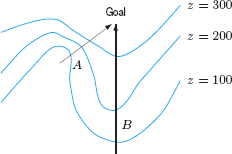
27. Figure 8.29 shows a contour map of a hill with two paths, A and B.
(a) On which path, A or B, will you have to climb more steeply?
(b) On which path, A or B, will you probably have a better view of the surrounding countryside? (Assume trees do not block your view.)
(c) Alongside which path is there more likely to be a stream?
28. Figure 8.30 shows cardiac output (in liters per minute) in patients suffering from shock as a function of blood pressure in the central veins (in mm Hg) and the time in hours since the onset of shock.4

(a) In a patient with blood pressure of 4 mm Hg, what is cardiac output when the patient first goes into shock? Estimate cardiac output three hours later. How much time has passed when cardiac output is reduced to 50% of the initial value?
(b) In patients suffering from shock, is cardiac output an increasing or decreasing function of blood pressure?
(c) Is cardiac output an increasing or decreasing function of time, t, where t represents the elapsed time since the patient went into shock?
(d) If blood pressure is 3 mm Hg, explain how cardiac output changes as a function of time. In particular, does it change rapidly or slowly during the first two hours of shock? During hours 2 to 4? During the last hour of the study? Explain why this information is useful to a physician treating a patient for shock.
29. The cornea is the front surface of the eye. Corneal specialists use a TMS, or Topographical Modeling System, to produce a “map” of the curvature of the eye's surface. A computer analyzes light reflected off the eye and draws level curves joining points of constant curvature. The regions between these curves are colored different colors.
The first two pictures in Figure 8.31 are cross-sections of eyes with constant curvature, the smaller being about 38 units and the larger about 50 units. For contrast, the third eye has varying curvature.
(a) Describe in words how the TMS map of an eye of constant curvature will look.
(b) Draw the TMS map of an eye with the cross-section in Figure 8.32. Assume the eye is circular when viewed from the front, and the cross-section is the same in every direction. Put reasonable numeric labels on your level curves.
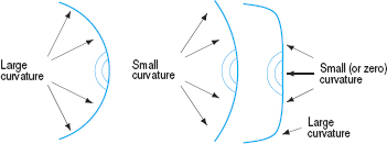
Figure 8.31: Pictures of eyes with different curvature

30. The power P produced by a windmill is proportional to the square of the diameter d of the windmill and to the cube of the speed v of the wind.5
(a) Write a formula for P as a function of d and v.
(b) A windmill generates 100 kW of power at a certain wind speed. If a second windmill is built having twice the diameter of the original, what fraction of the original wind speed is needed by the second windmill to produce 100 kW?
(c) Sketch a contour diagram for P.
31. Antibiotics can be toxic in large doses. If repeated doses of an antibiotic are to be given, the rate at which the medicine is excreted through the kidneys should be monitored by a physician. One measure of kidney function is the glomerular filtration rate, or GFR, which measures the amount of material crossing the outer (or glomerular) membrane of the kidney, in milliliters per minute. A normal GFR is about 125 ml/min. Figure 8.33 gives a contour diagram of the percent, P, of a dose of mezlocillin (an antibiotic) excreted, as a function of the patient's GFR and the time, t, in hours since the dose was administered.6
(a) In a patient with a GFR of 50, approximately how long will it take for 30% of the dose to be excreted?
(b) In a patient with a GFR of 60, approximately what percent of the dose has been excreted after 5 hours?
(c) Explain how we can tell from the graph that, for a patient with a fixed GFR, the amount excreted changes very little after 12 hours.
(d) Is the percent excreted an increasing or decreasing function of time? Explain why this makes sense.
(e) Is the percent excreted an increasing or decreasing function of GFR? Explain what this means to a physician giving antibiotics to a patient with kidney disease.

32. Each contour diagram (a) and (b) shows satisfaction with quantities of two items X and Y combined. Match (a) and (b) with the items in (I) and (II).
(a)

(b)

(I) X: Hours worked; Y: Time spent commuting
(II) X: Hourly wage; Y: Time for leisure
33. Each contour diagram (a) and (b) shows satisfaction with quantities of two items X and Y combined. Match (a) and (b) with the items in (I) and (II).
(a)

(b)

(I) X: Income; Y: Leisure time
(II) X: Income; Y: Hours worked
34. Figure 8.34 shows a contour plot of job satisfaction as a function of the hourly wage and the safety of the workplace. Match the jobs at points P, Q, and R with the three descriptions.
(a) The job is so unsafe that higher pay alone would not increase my satisfaction very much.
(b) I could trade a little less safety for a little more pay. It would not matter to me.
(c) The job pays so little that improving safety would not make me happier.

35. A shopper buys x units of item A and y units of item B, obtaining satisfaction s(x, y) from the purchase. (Satisfaction is called utility by economists.) The contours s(x, y) = xy = c are called indifference curves because they show pairs of purchases that give the shopper the same satisfaction.
(a) A shopper buys 8 units of A and 2 units of B. What is the equation of the indifference curve showing the other purchases that give the shopper the same satisfaction? Sketch this curve.
(b) After buying 4 units of item A, how many units of B must the shopper buy to obtain the same satisfaction as obtained from buying 8 units of A and 2 units of B?
(c) The shopper reduces the purchase of item A by k, a fixed number of units, while increasing the purchase of B to maintain satisfaction. In which of the following cases is the increase in B largest?
- Initial purchase of A is 6 units
- Initial purchase of A is 8 units
8.3 PARTIAL DERIVATIVES
In one-variable calculus we saw how the derivative measures the rate of change of a function. We begin by reviewing this idea.
Rate of Change of Airline Revenue
In Section 8.1 we saw a two-variable function which gives an airline's revenue, R, as a function of the number of full-price tickets, x, and the number of discount tickets, y, sold:
![]()
If we fix the number of discount tickets at y = 10, we have a one-variable function
![]()
The rate of the change of revenue with respect to x is given by the one-variable derivative
![]()
This tells us that, if y is fixed at 10, then the revenue increases by $350 for the next additional full-price ticket sold. We call g′(x) the partial derivative of R with respect to x at the point (x, 10). If R = f(x, y), we write
![]()
| Example 1 | Find the rate of change of revenue, R, as y increases with x fixed at x = 20. |
| Solution | Substituting x = 20 into R = 350x + 200y gives the one-variable function
The rate of change of R as y increases with x fixed is
|
We call ∂R/∂y = fy(20, y) the partial derivative of R with respect to y at the point (20, y). The fact that both partial derivatives of R are positive corresponds to the fact that the revenue is increasing as more of either type of ticket is sold.
Definition of the Partial Derivative
For any function f(x, y) we study the influence of x and y separately on the value f(x, y) by keeping one fixed and letting the other vary. The method of the previous example allows us to calculate the rates of change of f(x, y) with respect to x and y. For all points (a, b) at which the limits exist, we make the following definitions:
Partial Derivatives of f with Respect to x and y
The partial derivative of f with respect to x at (a, b) is the derivative of f with y fixed at b:
![]()
The partial derivative of f with respect to y at (a, b) is the derivative of f with x fixed at a:
![]()
If we think of a and b as variables, a = x and b = y, we have the partial derivative functions fx(x, y) and fy(x, y).
Just as with ordinary derivatives, there is an alternative notation:
Alternative Notation for Partial Derivatives
If z = f(x, y) we can write
![]()
![]()
We use the symbol ∂ to distinguish partial derivatives from ordinary derivatives. In cases where the independent variables have names different from x and y, we adjust the notation accordingly. For example, the partial derivatives of f(u, v) are denoted by fu and fv.
Estimating Partial Derivatives from a Table
| Example 2 | An experiment7 done on rats to measure the toxicity of formaldehyde yielded the data shown in Table 8.5. The values in the table show the percent, P, of rats that survived an exposure with concentration c (in parts per million) after t months, so P = f(t, c). Using Table 8.5, estimate ft(18, 6) and fc(18,6). Interpret your answers in terms of formaldehyde toxicity.
Table 8.5 Percent, P, of rat population surviving after exposure to formaldehyde vapor
|
| Solution | For ft(18, 6), we fix c at 6 ppm, and find the rate of change of percent surviving, P, with respect to t. We have
This is the rate of change of percent surviving, P, in the time t direction at the point (18, 6). The fact that it is negative means that P is decreasing as we read across the c = 6 row of the table in the direction of increasing t (that is, horizontally from left to right in Table 8.5). For fc(18, 6), we fix t at 18, and calculate the rate of change of P as we move in the direction of increasing c (that is, from top to bottom in Table 8.5). We have
The rate of change of P as c increases is about −1.22% per ppm. This means that as the concentration increases by 1 ppm from 6 ppm, the percent surviving 18 months decreases by about 1.22% per unit increase ppm. The partial derivative is negative because fewer rats survive this long when the concentration of formaldehyde increases. (That is, P goes down as c goes up.) |

Using Partial Derivatives to Estimate Values of the Function
| Example 3 | Use Table 8.5 and partial derivatives to estimate the percent of rats surviving if they are exposed to formaldehyde with a concentration of
(a) 6 ppm for 18.5 months (b) 18 ppm for 24 months (c) 9 ppm for 20.5 months |
| Solution | (a) Since t = 18.5 and c = 6, we want to evaluate P = f(18.5,6). Table 8.5 tells us that f(18,6) = 93% and we have just calculated
This partial derivative tells us that after 18 months of exposure to formaldehyde at a concentration of 6 ppm, P decreases by 1.5% for every additional month of exposure. Therefore after an additional 0.5 month, we have
(b) Now we wish to evaluate f(24,18). The closest entry to this in Table 8.5 is f(24,15) = 36. We keep t fixed at 24 and increase c from 15 to 18. We estimate the rate of change in P as c changes; this is ∂P/∂c. We see from Table 8.5 that
The percent surviving 24 months goes down from 36% by about 4.89% for one unit increase in the formaldehyde concentration above 15 ppm. We have:
We estimate that only about 21% of the rats would survive for 24 months if they were exposed to formaldehyde as strong as 18 ppm. Since this figure is an extrapolation from the available data, we should use it with caution. (c) To estimate f(20.5, 9), we use the closest entry f(20, 6) = 90. As we move from (20,6) to (20.5,9), the percentage, P, changes both due to the change in t and due to the change in c. We estimate the two partial derivatives at t = 20, c = 6:
The change in P due to a change of Δt = 0.5 month and Δc = 3 ppm is
So for t = 20.5, c = 9 we have
|


In Example 3(c), we used the relationship among ΔP, Δt, and Δc. In general, the relationship between the change Δf, in function value f(x, y) and the changes Δx and Δy is as follows:
Local Linearity

Estimating Partial Derivatives from a Contour Diagram
If we move parallel to one of the axes on a contour diagram, the partial derivative is the rate of change of the value of the function on the contours. For example, if the values on the contours are increasing in the direction of positive change, then the partial derivative must be positive.
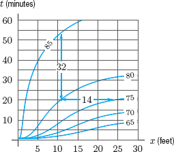
| Example 4 | Figure 8.35 shows the contour diagram for the temperature H(x, t) (in °F) in a room as a function of distance x (in feet) from a heater and time t (in minutes) after the heater has been turned on. What are the signs of Hx(10, 20) and Ht(10, 20)? Estimate these partial derivatives and explain the answers in practical terms.
|
| Solution | The point (10, 20) is on the H = 80 contour. As x increases, we move toward the H = 75 contour, so H is decreasing and Hx(10,20) is negative. This makes sense because as we move further from the heater, the temperature drops. On the other hand, as t increases, we move toward the H = 85 contour, so H is increasing and Ht(10, 20) is positive. This also makes sense, because it says that as time passes, the room warms up.
To estimate the partial derivatives, use a difference quotient. Looking at the contour diagram, we see there is a point on the H = 75 contour about 14 units to the right of (10,20). Hence, H decreases by 5 when x increases by 14, so the rate of change of H with respect to x is about ΔH/Δx = −5/14 ≈ −0.36. Thus, we find This means that near the point 10 feet from the heater, after 20 minutes the temperature drops about 1/3 of a degree for each foot we move away from the heater. To estimate Ht(10, 20), we look again at the contour diagram and notice that the H = 85 contour is about 32 units directly above the point (10, 20). So H increases by 5 when t increases by 32. Hence,
This means that after 20 minutes the temperature is going up about 1/6 of a degree in one more minute at the point 10 ft from the heater. |
Using Units to Interpret Partial Derivatives
The units of the independent and dependent variables can often be helpful in explaining the meaning of a partial derivative.
| Example 5 | Suppose that your weight w in pounds is a function f(c, n) of the number c of calories you consume daily and the number n of minutes you exercise daily. Using the units for w, c and n, interpret in everyday terms the statements
|
| Solution | The units of ∂w/∂c are pounds per calorie. The statement
means that if you are presently consuming 2000 calories daily and exercising 15 minutes daily, you will weigh about 0.02 pounds more for one more calorie you consume daily, or about 2 pounds for an extra 100 calories per day. The units of ∂w/∂n are pounds per minute. The statement
means that for the same calorie consumption and number of minutes of exercise, you will weigh about 0.025 pounds less for one extra minute you exercise daily, or about 1 pound less for an extra 40 minutes per day. So if you eat an extra 100 calories each day and exercise about 80 minutes more each day, your weight should remain roughly steady. |
Problems for Section 8.3
1. Using the contour diagram for f(x, y) in Figure 8.36, decide whether each of these partial derivatives is positive, negative, or approximately zero.
(a) fx (4, 1)
(b) fy (4, 1)
(c) fx(5, 2)
(d) fy(5, 2)

2. According to the contour diagram for f(x, y) in Figure 8.36, which is larger: fx(3, 1) or fx(5, 2)? Explain.
For Problems 3–4 refer to Table 8.4 on page 362 giving the heat index, I, in °F, as a function f (H, T) of the relative humidity, H, and the temperature, T, in °F. The heat index is a temperature which tells you how hot it feels as a result of the combination of humidity and temperature.
3. Estimate ∂I/∂H and ∂I/∂T for typical weather conditions in Tucson in summer (H = 10, T = 100). What do your answers mean in practical terms for the residents of Tucson?
4. Answer the question in Problem 3 for Boston in summer (H = 50, T = 80).
5. The demand for coffee, Q, in pounds sold per week, is a function of the price of coffee, c, in dollars per pound and the price of tea, t, in dollars per pound, so Q = f(c, t).
(a) Do you expect fc to be positive or negative? What about ft? Explain.
(b) Interpret each of the following statements in terms of the demand for coffee:
![]()
6. A drug is injected into a patient's blood vessel. The function c = f(x, t) represents the concentration of the drug at a distance x mm in the direction of the blood flow measured from the point of injection and at time t seconds since the injection. What are the units of the following partial derivatives? What are their practical interpretations? What do you expect their signs to be?
(a) ![]()
(b) ![]()
7. The quantity Q (in pounds) of beef that a certain community buys during a week is a function Q = f(b, c) of the prices of beef, b, and chicken, c, during the week. Do you expect ∂Q/∂b to be positive or negative? What about ∂Q/∂c?
8. Table 8.6 gives the number of calories burned per minute, B = f(s, w), for someone roller-blading,8 as a function of the person's weight, w, and speed, s.
(a) Is fw positive or negative? Is fs positive or negative? What do your answers tell us about the effect of weight and speed on calories burned per minute?
(b) Estimate fw(160, 10) and fs(160, 10). Interpret your answers.

9. Estimate zx(1, 0) and zx(0,1) and zy(0,1) from the contour diagram for z(x, y) in Figure 8.37.

10. The monthly mortgage payment in dollars, P, for a house is a function of three variables:
![]()
where A is the amount borrowed in dollars, r is the interest rate, and N is the number of years before the mortgage is paid off.
(a) f(92000,14,30) = 1090.08. What does this tell you, in financial terms?
(b) ![]() = 72.82. What is the financial significance of the number 72.82?
= 72.82. What is the financial significance of the number 72.82?
(c) Would you expect ∂P/∂A to be positive or negative? Why?
(d) Would you expect ∂P/∂N to be positive or negative? Why?
11. The sales of a product, S = f(p, a), are a function of the price, p, of the product (in dollars per unit) and the amount, a, spent on advertising (in thousands of dollars).
(a) Do you expect fp to be positive or negative? Why?
(b) Explain the meaning of the statement fa(8, 12) = 150 in terms of sales.
12. Figure 8.13 on page 360 gives a contour diagram of corn production as a function of rainfall, R, in inches and temperature, T, in °F. Corn production, C, is measured as a percentage of the present production, and C = f(R, T). Estimate the following quantities. Give units and interpret your answers in terms of corn production:
(a) fR(15, 76)
(b) fT(15, 76)
13. Figure 8.38 shows a contour diagram for the monthly payment P as a function of the interest rate, r%, and the amount, L, of a 5-year loan. Estimate ∂P/∂r and ∂P/∂L at the point where r = 8 and L = 5000. Give the units and the financial meaning of your answers.

14. Use the diagram from Problem 14 in Section 8.1, to estimate HT(T, w) for T = 10, 20, 30 and w = 0.1, 0.2, 0.3. What is the practical meaning of these partial derivatives?
15. People commuting to a city can choose to go either by bus or by train. The number of people who choose either method depends in part upon the price of each. Let f(P1, P2) be the number of people who take the bus when P1 is the price of a bus ride and P2 is the price of a train ride. What can you say about the signs of ∂f/∂P1 and ∂f/∂P2? Explain your answers.
16. Suppose that x is the price of one brand of gasoline and y is the price of a competing brand. Then q1, the quantity of the first brand sold in a fixed time period, depends on both x and y, so q1 = f(x, y). Similarly, if q2 is the quantity of the second brand sold during the same period, q2 = g(x, y). What do you expect the signs of the following quantities to be? Explain.
(a) ∂q1/∂x and ∂q2/∂y
(b) ∂q1/∂y and ∂q2/∂x
17. An airline's revenue, R, is a function of the number of full-price tickets, x, and the number of discount tickets, y, sold. Values of R = f(x, y) are in Table 8.1 on page 354.
(a) Evaluate f(200, 400), and interpret your answer.
(b) Is fx(200,400) positive or negative? Is fy(200,400) positive or negative? Explain.
(c) Estimate the partial derivatives in part (b). Give units and interpret your answers in terms of revenue.
18. In Problem 17 the revenue is $150,000 when 200 full-price tickets and 400 discount tickets are sold; that is, f(200, 400) = 150,000. Use this fact and the partial derivatives fx(200, 400) = 350 and fy(200, 400) = 200 to estimate the revenue when
(a) x = 201 and y = 400
(b) x = 200 and y = 405
(c) x = 203 and y = 406
19. For a function f(x, y), we are given f(100, 20) = 2750, and fx(100, 20) = 4, and fy(100, 20) = 7. Estimate f(105, 21).
20. For a function f(r, s), we are given f(50, 100) = 5.67, and fr(50,100) = 0.60, and fs(50,100) = −0.15. Estimate f(52, 108).
21. Table 8.5 on page 370 gives the percent of rats surviving, P, as a function of time, t, in months and concentration of formaldehyde, c, in ppm, so P = f(t, c). Use partial derivatives to estimate the percent surviving after 26 months when the concentration is 15.
22. The cardiac output, represented by c, is the volume of blood flowing through a person's heart per unit time. The systemic vascular resistance (SVR), represented by s, is the resistance to blood flowing through veins and arteries. Let p be a person's blood pressure. Then p is a function of c and s, so p = f(c, s).
(a) What does ∂p/∂c represent?
Suppose now that p = kcs, where k is a constant.
(b) Sketch the level curves of p. What do they represent? Label your axes.
(c) For a person with a weak heart, it is desirable to have the heart pumping against less resistance, while maintaining the same blood pressure. Such a person may be given the drug nitroglycerine to decrease the SVR and the drug Dopamine to increase the cardiac output. Represent this on a graph showing level curves. Put a point A on the graph representing the person's state before drugs are given and a point B for after.
(d) Right after a heart attack, a patient's cardiac output drops, thereby causing the blood pressure to drop. A common mistake made by medical residents is to get the patient's blood pressure back to normal by using drugs to increase the SVR, rather than by increasing the cardiac output. On a graph of the level curves of p, put a point D representing the patient before the heart attack, a point E representing the patient right after the heart attack, and a third point F representing the patient after the resident has given the drugs to increase the SVR.
23. In each case, give a possible contour diagram for the function f(x, y) if
(a) fx > 0 and fy > 0
(b) fx > 0 and fy < 0
(c) fx < 0 and fy > 0
(d) fx < 0 and fy < 0
24. Figure 8.39 shows contours of f(x, y) with values of f on the contours omitted. If fx(P) > 0, find the sign of
(a) fy(P)
(b) fy(Q)
(c) fx(Q)

25. Figure 8.40 shows a contour diagram of Dan's happiness with snacks of different numbers of cherries and grapes.
(a) What is the slope of the contours?
(b) What does the slope tell you?

8.4 COMPUTING PARTIAL DERIVATIVES ALGEBRAICALLY
The partial derivative fx(x, y) is the ordinary derivative of the function f(x, y) with respect to x with y fixed, and the partial derivative fy(x, y) is the ordinary derivative of f(x, y) with respect to y with x fixed. Thus, we can use all the techniques for differentiation from single-variable calculus to find partial derivatives.
| Example 1 | Let f(x, y) = x2 + 5y2. Find fx(3, 2) and fy(3, 2) algebraically. |
| Solution | We use the fact that fx(3, 2) is the derivative of f(x, 2) at x = 3. To find fx, we fix y at 2:
Differentiating with respect to x gives
Similarly, fy(3, 2) is the derivative of f(3, y) at y = 2. To find fy, we fix x at 3:
Differentiating with respect to y, we have
|
| Example 2 | Let f(x, y) = x2 + 5y2 as in Example 1. Find fx and fy as functions of x and y. |
| Solution | To find fx, we treat y as a constant. Thus 5y2 is a constant and the derivative with respect to x of this term is 0. We have
To find fy, we treat x as a constant and so the derivative of x2 with respect to y is zero. We have
|
| Example 4 | The concentration C of bacteria in the blood (in millions of bacteria/ml) following the injection of an antibiotic is a function of the dose x (in gm) injected and the time t (in hours) since the injection. Suppose we are told that C = f(x, t) = te−xt. Evaluate the following quantities and explain what each one means in practical terms: (a) fx (1, 2) (b) ft(1, 2) |
| Solution | (a) To find fx, we treat t as a constant and differentiate with respect to x, giving
Substituting x = 1, t = 2 gives
To see what fx(1, 2) means, think about the function f(x, 2) of which it is the derivative. The graph of f(x, 2) in Figure 8.41 gives the concentration of bacteria as a function of the dose two hours after the injection. The derivative fx(1, 2) is the slope of this graph at the point x = 1; it is negative because a larger dose reduces the bacteria population. More precisely, the partial derivative fx(1, 2) gives the rate of change of bacteria concentration with respect to the dose injected, namely a decrease in bacteria concentration of 0.54 million/ml per gram of additional antibiotic injected. (b) To find ft, treat x as a constant and differentiate using the product rule:
Substituting x = 1, t = 2 gives
To see what ft(1, 2) means, think about the function f(1, t) of which it is the derivative. The graph of f(1, t) in Figure 8.42 gives the concentration of bacteria at time t if the dose of antibiotic is 1 gm. The derivative ft(1, 2) is the slope of the graph at the point t = 2; it is negative because after 2 hours the concentration of bacteria is decreasing. More precisely, the partial derivative ft(1, 2) gives the rate at which the bacteria concentration is changing with respect to time, namely a decrease in bacteria concentration of 0.14 million/ml per hour. Figure 8.41: Bacteria concentration after 2 hours as a function of the quantity of antibiotic injected
Figure 8.42: Bacteria concentration as a function of time if 1 unit of antibiotic is injected |


| Example 5 | Let's consider a small printing business where N is the number of workers, V is the value of the equipment (in units of $25,000), and P is the production, measured in thousands of pages per day. Suppose the production function for this company is given by
(a) If this company has a labor force of 100 workers and 200 units' worth of equipment, what is the production output of the company? (b) Find fN(100, 200) and fV(100, 200). Interpret your answers in terms of production. |
| Solution | (a) We have N = 100 and V = 200, so
(b) To find fN, we treat V as a constant and differentiate with respect to N:
Substituting N = 100, V = 200 gives
This tells us that if we have 200 units of equipment and increase the number of workers by 1 from 100 to 101, the production output will go up by about 1.58 units, or 1580 pages per day. Similarly, to find fV(100, 200), we treat N as a constant and differentiate with respect to V:
Substituting N = 100, V = 200 gives
This tells us that if we have 100 workers and increase the value of the equipment by 1 unit ($25,000) from 200 units to 201 units, the production goes up by about 0.53 units, or 530 pages per day. |
Second-Order Partial Derivatives
Since the partial derivatives of a function are themselves functions, we can usually differentiate them, giving second-order partial derivatives. A function z = f(x, y) has two first-order partial derivatives, fx and fy, and four second-order partial derivatives.
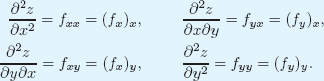
It is usual to omit the parentheses, writing fxy instead of (fx)y and ![]() instead of
instead of ![]() .
.
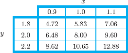
| Example 6 | Use the values of the function f(x, y) in Table 8.7 to estimate fxy(1, 2) and fyx(1, 2).
|
| Solution | Since fxy = (fx)y, we first estimate fx:
Thus,
Similarly,
Observe that in this example, fxy = fyx at the point (1, 2). |


| Example 7 | Compute the four second-order partial derivatives of f(x, y) = xy2 + 3x2ey. |
| Solution | From fx(x, y) = y2 + 6xey we get
From fy(x, y) = 2xy + 3x2ey we get
Observe that fxy = fyx in this example. |
The Mixed Partial Derivatives Are Equal
It is not an accident that the estimates for fxy(1, 2) and fyx(1,2) are equal in Example 6, because the same values of the function are used to calculate each one. The fact that fxy = fyx in Example 7 corroborates the following general result:
If fxy and fyx are continuous at (a, b), then
![]()
Most of the functions we will encounter not only have fxy and fyx continuous, but all their higher-order partial derivatives (such as fxxy or fxyyy) will be continuous. We call such functions smooth.
Problems for Section 8.4
Find the partial derivatives in Problems 1–13. The variables are restricted to a domain on which the function is defined.
1. fx and fy if f(x, y) = x2 + 2xy + y3
2. fx and fy if f(x, y) = 2x2 + 3y2
3. fx and fy if f(x, y) = 100x2y
4. fu and fv if f(u, v) = u2 + 5uv + v2
5. ![]()
6. ![]()
7. ft if f(t, a) = 5a2t3
8. fx and fy if f(x, y) = 5x2y3 + 8xy2 − 3x2
9. fx and fy if f(x, y) = 10x2e3y
10. zx if z = x2y + 2x5y
11. ![]()
12. ![]()
13. ![]()
14. If f(x, y) = x3 + 3y2, find f(1, 2), fx(1, 2), fy(1, 2).
15. If f(u, v) = 5uv2, find f(3, 1), fu(3, 1), and fv(3, 1).
16. Figure 8.43 is a contour diagram of f(x, y). In each of the following cases, list the marked points in the diagram (there may be none or more than one) at which
(a) fx < 0
(b) fy > 0
(c) fxx > 0
(d) fyy < 0

17. (a) Let f(x, y) = x2 + y2. Estimate fx(2, 1) and fy(2, 1) using the contour diagram for f in Figure 8.44.
(b) Estimate fx (2,1) and fy (2, 1) from a table of values for f with x = 1.9, 2, 2.1 and y = 0.9,1, 1.1.
(c) Compare your estimates in parts (a) and (b) with the exact values of fx(2, 1) and fy(2, 1) found algebraically.

18. The amount of money, $B, in a bank account earning interest at a continuous rate, r, depends on the amount deposited, $P, and the time, t, it has been in the bank, where
![]()
Find ∂B/∂t, ∂B/∂r and ∂B/∂P and interpret each in financial terms.
19. A company's production output, P, is given in tons, and is a function of the number of workers, N, and the value of the equipment, V, in units of $25,000. The production function for the company is
![]()
The company currently employs 80 workers, and has equipment worth $750,000. What are N and V? Find the values of f, fN, and fV at these values of N and V. Give units and explain what each answer means in terms of production.
20. The cost of renting a car from a certain company is $40 per day plus 15 cents per mile, and so we have
![]()
Find ∂C/∂d and ∂C/∂m. Give units and explain why your answers make sense.
For Problems 21–32, calculate all four second-order partial derivatives and confirm that the mixed partials are equal.
21. f(x, y) = x2y
22. f(x, y) = xey
23. f(x, y) = x2 +2xy+y2
24. ![]()
25. f = 5 + x2y2
26. f = exy
27. B = 5xe−2t
28. f(x, t) = t3 − 4x2t
29. f = 100ert
30. ![]()
31. V = πr2h
32. P = 2KL2
33. Is there a function f which has the following partial derivatives? If so what is it? Are there any others?
![]()
34. Show that the Cobb-Douglas function
![]()
satisfies the equation
![]()
Problems 35–37 are about the money supply, M, which is the total value of all the cash and checking account balances in an economy. It is determined by the value of all the cash, B, the ratio, c, of cash to checking deposits, and the fraction, r, of checking account deposits that banks hold as cash:
![]()
(a) Find the partial derivative.
(b) Give its sign.
(c) Explain the significance of the sign in practical terms.
35. ∂M/∂B
36. ∂M/∂r
37. ∂M/∂c
8.5 CRITICAL POINTS AND OPTIMIZATION
To optimize a function means to find the largest or smallest value of the function. If the function represents profit, we may want to find the conditions that maximize profit. On the other hand, if the function represents cost, we may want to find the conditions that minimize cost. In Chapter 4, we saw how to optimize a function of one variable by investigating critical points. In this section, we see how to extend the notions of critical points and local extrema to a function of more than one variable.
Local and Global Maxima and Minima for Functions of Two Variables
Functions of several variables, like functions of one variable, can have local and global extrema (that is, local and global maxima and minima). A function has a local extremum at a point where it takes on the largest or smallest value in a small region around the point. Global extrema are the largest or smallest value anywhere. For a function f defined on a domain R, we say:
- f has a local maximum at P0 if f(P0) ≥ f(P) for all points P near P0
- f has a local minimum at P0 if f(P0) ≤ f(P) for all points P near P0
- f has a global maximum at P0 if f(P0) ≥ f(P) for all points P in R
- f has a global minimum at P0 if f(P0) ≤ f(P) for all points P in R
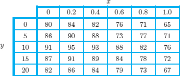
| Example 1 | Table 8.8 gives a table of values for a function f(x, y). Estimate the location and value of any global maxima or minima for 0 ≤ x ≤ 1 and 0 ≤ y ≤ 20. |
| Solution | The global maximum value of the function appears to be 95 at the point (0.2,10). Since the table only gives certain values, we cannot be sure that this is exactly the maximum. (The function might have a larger value at, for example, (0.3,11).) The global minimum value of this function on the points given is 65 at the point (1,0). |
| Example 2 | Figure 8.45 gives a contour diagram for a function f(x, y). Estimate the location and value of any local maxima or minima. Are any of these global maxima or minima on the square shown?
Figure 8.45: Where are the local and global extreme points of this function? |
| Solution | There is a local maximum of above 8 near the point (6, 5), a local maximum of above 6 near the point (2, 6), and a local minimum of below 3 near the point (3, 2). The value above 8 is the global maximum and the value below 3 is the global minimum on the given domain. |

In Example 1 and Example 2, we can estimate the location and value of extreme points, but we do not have enough information to find them exactly. This is usually true when we are given a table of values or a contour diagram. To find local or global extrema exactly, we usually need to have a formula for the function.
Finding a Local Maximum or Minimum Analytically
In one-variable calculus, the local extrema of a function occur at points where the derivative is zero or undefined. How does this generalize to the case of functions of two or more variables? Suppose that a function f(x, y) has a local maximum at a point (x0, y0) which is not on the boundary of the domain of f. If the partial derivative fx(x0, y0) were defined and positive, then we could increase f by increasing x. If fx(x0, y0) < 0, then we could increase f by decreasing x. Since f has a local maximum at (x0, y0), there can be no direction in which f is increasing, so we must have fx(x0, y0) = 0. Similarly, if fy(x0, y0) is defined, then fy(x0, y0) = 0. The case in which f(x, y) has a local minimum is similar. Therefore, we arrive at the following conclusion:
If a function f(x, y) has a local maximum or minimum at a point (x0, y0) not on the boundary of the domain of f, then either
![]()
or (at least) one partial derivative is undefined at the point (x0, y0). Points where each of the partial derivatives is either zero or undefined are called critical points.
As in the single-variable case, the fact that (x0, y0) is a critical point for f does not necessarily mean that f has a maximum or a minimum there.
How Do We Find Critical Points?
To find critical points of a function f, we find the points where both partial derivatives of f are zero or undefined.
| Example 3 | Find and analyze the critical points of f(x, y) = x2 − 2x + y2 − 4y + 5. |
| Solution | To find the critical points, we set both partial derivatives equal to zero:
Solving these equations gives x = 1 and y = 2. Hence, f has only one critical point, namely (1, 2). What is the behavior of f near (1, 2)? The values of the function in Table 8.9 suggest that the function has a local minimum value of 0 at the point (1, 2). |
Table 8.9 Values of f(x, y) near the point (1, 2)

| Example 4 | A manufacturing company produces two products which are sold in two separate markets. The company's economists analyze the two markets and determine that the quantities, q1 and q2, demanded by consumers and the prices, p1 and p2 (in dollars), of each item are related by the equations
Thus, if the price for either item increases, the demand for it decreases. The company's total production cost is given by
If the company wants to maximize its total profits, how much of each product should it produce? What is the maximum profit?9 |
| Solution | The total revenue R is the sum of the revenues, p1q1 and p2q2, from each market. Substituting for p1 and p2, we get
Thus the total profit π is given by
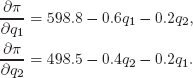
To maximize π, we compute partial derivatives:
Since the partial derivatives are defined everywhere, the only critical points of π are those where the partial derivatives of π are both equal to zero. Thus, we solve the equations for q1 and q2,
giving
To see whether this is a maximum, we look at a table of values of profit π around this point. Table 8.10 suggests that profit is greatest at (699,897). So the company should produce 699 units of the first product priced at $390.30 per unit, and 897 units of the second product priced at $320.60 per unit. The maximum profit is then π(699,897) = $432,797. |


Is a Critical Point a Local Maximum or a Local Minimum?
We can often see whether a critical point is a local maximum or minimum or neither by looking at a table or contour diagram. The following analytic method may also be useful in distinguishing between local maxima and minima.10 It is analogous to the Second Derivative Test in Chapter 4.
Second Derivative Test for Functions of Two Variables
Suppose (x0, y0) is a critical point where fx(x0, y0) = fy(x0, y0) = 0. Let
![]()
- If D > 0 and fxx(x0, y0) > 0, then f has a local minimum at (x0, y0).
- If D > 0 and fxx(x0, y0) < 0, then f has a local maximum at (x0, y0).
- If D < 0, then we say f has a saddle point at (x0, y0).
- If D = 0, the test is inconclusive.
If (x0, y0) is a saddle point of f, then it is neither a local maximum nor a local minimum of f. Figure 8.46 gives a contour diagram of a function f around a saddle point. As we move in the y-direction from the center of the diagram, the value of f decreases; but as we move in the x-direction from the center, the value of f increases.
| Example 5 | Use the second derivative test to confirm that the critical point q1 = 699.1, q2 = 896.7 gives a local maximum of the profit function π of Example 4. |
| Solution | To see whether or not we have found a maximum point, we compute the second-order partial derivatives:
Since
and
the second derivative test implies that we have found a local maximum point. |
Problems for Section 8.5
1. Figure 8.47 shows contours of f(x, y). List the x- and y-coordinates and the value of the function at any local maximum and local minimum points, and identify which is which. Are any of these local extrema also global extrema on the region shown? If so, which ones?

2. Figure 8.48 shows contours of f(x, y). List x- and y-coordinates and the value of the function at any local maximum and local minimum points, and identify which is which. Are any of these local extrema also global extrema on the region shown? If so, which ones?

In Problems 3–5, estimate the position and approximate value of the global maxima and minima on the region shown.
3.

4.

5.

In Problems 6–15, find all the critical points and determine whether each is a local maximum, local minimum, a saddle point, or none of these.
6. f(x, y) = x2 + 4x + y2
7. f(x, y) = x2 + xy + 3y
8. f(x, y) = x2 + y2 + 6x −10y + 8
9. f(x, y) = y3 − 3xy + 6x
10. f(x, y) = x3 + y2 − 3x2 + 10y + 6
11. f(x, y) = x3 + y3 − 6y2 − 3x + 9
12. f(x, y) = x3 + y3 − 3x2 − 3y + 10
13. f(x, y) = x2 − 2xy + 3y2 − 8y
14. f(x, y) = x3 − 3x + y3 − 3y
15. f(x, y) = 400 − 3x2 − 4x + 2xy − 5y2 + 48y
16. By looking at the weather map in Figure 8.5 on page 358, find the maximum and minimum daily high temperatures in the states of Mississippi, Alabama, Pennsylvania, New York, California, Arizona, and Massachusetts.
17. For f(x, y) = A − (x2 + Bx + y2 + Cy), what values of A, B, and C give f a local maximum value of 15 at the point (−2,1)?
18. A missile has a guidance device which is sensitive to both temperature, t°C, and humidity, h. The range in km over which the missile can be controlled is given by
![]()
What are the optimal atmospheric conditions for controlling the missile?
19. The quantity of a product demanded by consumers is a function of its price. The quantity of one product demanded may also depend on the price of other products. For example, if the only chocolate shop in town (a monopoly) sells milk and dark chocolates, the price it sets for each affects the demand of the other. The quantities demanded, q1 and q2, of two products depend on their prices, p1 and p2, as follows:
![]()
(a) What does the fact that the coefficients of p1 and p2 are negative tell you? Give an example of two products that might be related this way.
(b) If one manufacturer sells both products, how should the prices be set to generate the maximum possible revenue? What is that maximum possible revenue?
20. Two products are manufactured in quantities q1 and q2 and sold at prices of p1 and p2, respectively. The cost of producing them is given by
![]()
(a) Find the maximum profit that can be made, assuming the prices are fixed.
(b) Find the rate of change of that maximum profit as p1 increases.
21. A company operates two plants which manufacture the same item and whose total cost functions are
![]()
where q1 and q2 are the quantities produced by each plant. The company is a monopoly. The total quantity demanded, q = q1 + q2, is related to the price, p, by
![]()
How much should each plant produce in order to maximize the company's profit?11
8.6 CONSTRAINED OPTIMIZATION
Many real optimization problems are constrained by external circumstances. For example, a city wanting to build a public transportation system has a limited number of tax dollars available. A nation trying to maintain its balance of trade must spend less on imports than it earns on exports. In this section, we see how to find an optimum value under such constraints.
A Constrained Optimization Problem
Suppose we want to maximize the production of a company under a budget constraint. Suppose production, f, is a function of two variables, x and y, which are quantities of two raw materials, and
![]()
If x and y are purchased at prices of p1 and p2 dollars per unit, what is the maximum production f that can be obtained with a budget of c dollars?
To increase f without regard to the budget, we simply increase x and y. However, the budget prevents us from increasing x and y beyond a certain point. Exactly how does the budget constrain us? Suppose that x and y each cost $100 per unit, and suppose that the total budget is $378,000. The amount spent on x and y together is given by g(x, y) = 100x + 100y, and since we can't spend more than the budget allows, we must have:
![]()
The goal is to maximize the function
![]()
Since we expect to exhaust the budget, we have
![]()
| Example 1 | A company has production function f(x, y) = x2/3y1/3 and budget constraint 100x + 100y = 378,000.
(a) If $100,000 is spent on x, how much can be spent on y? What is the production in this case? (b) If $200,000 is spent on x, how much can be spent on y? What is the production in this case? (c) Which of the two options above is the better choice for the company? Do you think this is the best of all possible options? |
| Solution | (a) If the company spends $100,000 on x, then it has $278,000 left to spend on y. In this case, we have 100x = 100,000, so x = 1000, and 100y = 278,000, so y = 2780. Therefore,
(b) If the company spends $200,000 on x, then it has $178,000 left to spend on y. Therefore, x = 2000 and y = 1780, and so
(c) Of these two options, (b) is better since production is larger in this case. This is probably not optimal, since there are many other combinations of x and y that we have not checked. |
Graphical Approach: Maximizing Production Subject to a Budget Constraint
How can we find the maximum value of production? We maximize the objective function
![]()
subject to x ≥ 0 and y ≥ 0 and the budget constraint
![]()
The constraint is represented by the line in Figure 8.49. Any point on or below the line represents a pair of values of x and y that we can afford. A point on the line completely exhausts the budget, while a point below the line represents values of x and y which can be bought without using up the budget. Any point above the line represents a pair of values that we cannot afford.
Figure 8.49 also shows some contours of the production function f. Since we want to maximize f, we want to find the point which lies on the contour with the largest possible f value and which lies within the budget. The point we are looking for must lie on the budget constraint because we should spend all the available money. The key observation is this: The maximum occurs at a point P where the budget constraint is tangent to a production contour. (See Figure 8.49.) The reason is that if we are on the constraint line to the left of P, moving right on the constraint increases f; if we are on the line to the right of P, moving left increases f. Thus, the maximum value of f on the budget constraint line occurs at the point P.
In general, provided f and g are smooth, we have the following result:
If f(x, y) has a global maximum or minimum on the constraint g(x, y) = c, it occurs at a point where the graph of the constraint is tangent to a contour of f, or at an endpoint of the constraint.12

Figure 8.49: At the optimal point P the budget constraint is tangent to a production contour
Analytical Approach: The Method of Lagrange Multipliers
Suppose we want to optimize f(x, y) subject to the constraint g(x, y) = c. We make the following definition.
Suppose P0 is a point satisfying the constraint g(x, y) = c.
- f has a local maximum at P0 subject to the constraint if f(P0) ≥ f(P) for all points P near P0 satisfying the constraint.
- f has a global maximum at P0 subject to the constraint if f(P0) ≥ f(P) for all points P satisfying the constraint.
Local and global minima are defined similarly.
It can be shown13 that the constraint is tangent to a contour of f at the point which satisfies the equations laid out in the following method.
Method of Lagrange Multipliers To optimize f(x, y) subject to the constraint g(x, y) = c, solve the following system of three equations:
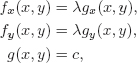
for the three unknowns x, y, and λ the number λ is called the Lagrange multiplier. If f has a constrained global maximum or minimum, then it occurs at one of the solutions (x0, y0) to this system or at an endpoint of the constraint.


The Meaning of λ
In the previous example, we never found (or needed) the value of λ. However, λ does have a practical interpretation. In the production problem we maximized
![]()
subject to the constraint
![]()
We solved the equations

to get x = 2520, y = 1260. Continuing to find λ gives us
![]()
Suppose now we do another, apparently unrelated calculation. Suppose our budget is increased by $1000, from $378,000 to $379,000. The new budget constraint is
![]()
The corresponding solution is at x = 2527, y = 1263 and the new maximum value (instead of f = 2000.1) is
![]()
The additional $1000 in the budget increased the production level f by 5.3 units. Notice that production increased by 5.3/1000 = 0.0053 units per dollar, which is our value of λ. The value of λ represents the extra production achieved by increasing the budget by one dollar—in other words, the extra “bang” you get for an extra “buck” of budget.
Solving for λ in either of the equations fx = λgx or fy = λgy suggests that the Lagrange multiplier is given by the ratio of the changes:
![]()
These results suggest the following interpretations of the Lagrange multiplier λ:
- The value of λ is approximately the change in the optimum value of f when the value of the constraint is increased by 1 unit.
- The value of λ represents the rate of change of the optimum value of f as the constraint increases.
| Example 3 | The quantity of goods produced according to the function f(x, y) = x2/3y1/3 is maximized subject to the budget constraint 100x + 100y = 378,000. Suppose the budget is increased to allow a small increase in production. What price must the product sell for if it is to be worth the increased budget? |
| Solution | We know that λ = 0.0053. Therefore, increasing the budget by $1 increases production by about 0.0053 unit. In order to make the increase in budget profitable, the extra goods produced must sell for more than $1. If the price is p in dollars, we must have 0.0053p > 1. Thus, we need p > 1/0.0053 ≈ $189. |
| Example 4 | If x and y are the amounts of raw materials used, the quantity, Q, of a product manufactured is
Assume that x costs $20 per unit, y costs $10 per unit, and the production budget is $10,000. (a) How many units of x and y should be purchased in order to maximize production? How many units are produced at that point? (b) Find the value of λ and interpret it. |
| Solution | (a) We maximize f(x, y) = xy subject to the constraint g(x, y) = 20x + 10y = 10,000 and x ≥ 0, y ≥ 0. We have the following partial derivatives:
The method of Lagrange multipliers gives the following equations:
Substituting values of x and y from the first two equations into the third gives
Substituting λ = 25 in the first two equations above gives x = 250 and y = 500. The endpoints of the constraint are the point (500,0) and (0,1000). Since
the maximum value of the production function is
The company should purchase 250 units of x and 500 units of y, giving 125,000 units of products. (b) We have λ = 25. This tells us that if the budget is increased by $1, we expect production to go up by about 25 units. If the budget goes up by $1000, maximum production will increase about 25,000 to a total of roughly 150,000 units. |


The Lagrangian Function
Constrained optimization problems are frequently solved using a Lagrangian function, ![]() . For example, to optimize the function f(x, y) subject to the constraint g(x, y) = c, we use the Lagrangian function
. For example, to optimize the function f(x, y) subject to the constraint g(x, y) = c, we use the Lagrangian function
![]()
To see why the function ![]() is useful, compute the partial derivatives of
is useful, compute the partial derivatives of ![]() :
:

Notice that if (x0, y0) gives a maximum or minimum value of f(x, y) subject to the constraint g(x, y) = c and λ0 is the corresponding Lagrange multiplier, then at the point (x0, y0, λ0), we have
![]()
In other words, (x0, y0, λ0) is a critical point for the unconstrained problem of optimization of the Lagrangian, ![]() (x, y, λ).
(x, y, λ).
We can therefore attack constrained optimization problems in two steps. First, write down the Lagrangian function ![]() . Second, find the critical points of
. Second, find the critical points of ![]() .
.
Problems for Section 8.6
In Problems 1–10, use Lagrange multipliers to find the maximum or minimum values of f (x, y) subject to the constraint.
1. f(x, y) = x + y, x2 + y2 = 1
2. f(x, y) = x2 + 4xy, x + y = 100
3. f(x, y) = xy, 5x + 2y = 100
4. f(x, y) = x2 + 3y2 + 100, 8x + 6y = 88
5. f(x, y) = 5xy, x + 3y = 24
6. f(x, y) = 3x − 2y, x2 + 2y2 = 44
7. f(x, y) = x2 + y, x2 − y2 = 1
8. f(x, y) = xy, 4x2 + y2 = 8
9. f(x, y) = x2 + y2, 4x − 2y = 15
10. f(x, y) = x2 + y2, x4 + y4 = 2
11. Figure 8.50 shows contours labeled with values of f(x, y) and a constraint g(x, y) = c. Mark the approximate points at which:
(a) f has a maximum
(b) f has a maximum on the constraint g = c.

12. Figure 8.51 shows contours of f(x, y) and the constraint g(x, y) = c. Approximately what values of x and y maximize f(x, y) subject to the constraint? What is the approximate value of f at this maximum?
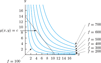
13. The quantity, Q, of a good produced depends on the quantities x1 and x2 of two raw materials used:
![]()
A unit of x1 costs $10, and a unit of x2 costs $25. We want to maximize production with a budget of $50 thousand for raw materials.
(a) What is the objective function?
(b) What is the constraint?
14. The quantity, Q, of a certain product manufactured depends on the quantity of labor, L, and of capital, K, used according to the function
![]()
Labor costs $100 per unit and capital costs $200 per unit. What combination of labor and capital should be used to produce 36,000 units of the goods at minimum cost? What is that minimum cost?
15. The Cobb-Douglas production function for a product is
![]()
where P is the quantity produced, L is the size of the labor force, and K is the amount of total equipment. Each unit of labor costs $300, each unit of equipment costs $100, and the total budget is $15,000.
(a) Make a table of L and K values which exhaust the budget. Find the production level, P, for each.
(b) Use the method of Lagrange multipliers to find the optimal way to spend the budget.
16. A firm manufactures a commodity at two different factories. The total cost of manufacturing depends on the quantities, q1 and q2, supplied by each factory, and is expressed by the joint cost function,
![]()
The company's objective is to produce 200 units, while minimizing production costs. How many units should be supplied by each factory?
17. The quantity, Q, of a product manufactured by a company is given by
![]()
where a is a positive constant, K is the quantity of capital and L is the quantity of labor used. Capital costs are $20 per unit, labor costs are $10 per unit, and the company wants costs for capital and labor combined to be no higher than $150. Suppose you are asked to consult for the company, and learn that 5 units each of capital and labor are being used.
(a) What do you advise? Should the company use more or less labor? More or less capital? If so, by how much?
(b) Write a one-sentence summary that could be used to sell your advice to the board of directors.
18. For a cost function, f(x, y), the minimum cost for a production of 50 is given by f(33, 87) = 1200, with λ = 15. Estimate the cost if the production quota is:
(a) Raised to 51
(b) Lowered to 49
19. A company has the production function P(x, y), which gives the number of units that can be produced for given values of x and y; the cost function C(x, y) gives the cost of production for given values of x and y.
(a) If the company wishes to maximize production at a cost of $50,000, what is the objective function f? What is the constraint equation? What is the meaning of λ in this situation?
(b) If instead the company wishes to minimize the costs at a fixed production level of 2000 units, what is the objective function f? What is the constraint equation? What is the meaning of λ in this situation?
20. You have set aside 20 hours to work on two class projects. You want to maximize your grade (measured in points), which depends on how you divide your time between the two projects.
(a) What is the objective function for this optimization problem and what are its units?
(b) What is the constraint?
(c) Suppose you solve the problem by the method of Lagrange multipliers. What are the units for λ?
(d) What is the practical meaning of the statement λ = 5?
21. A steel manufacturer can produce P(K, L) tons of steel using K units of capital and L units of labor, with production costs C(K, L) dollars. With a budget of $600,000, the maximum production is 2,500,000 tons, using $400,000 of capital and $200,000 of labor. The Lagrange multiplier is λ = 3.17.
(a) What is the objective function?
(b) What is the constraint?
(c) What are the units for λ?
(d) What is the practical meaning of the statement λ = 3.17?
22. The quantity, q, of a product manufactured depends on the number of workers, W, and the amount of capital invested, K, and is given by the Cobb-Douglas function
![]()
In addition, labor costs are $10 per worker and capital costs are $20 per unit and the budget is $3000.
(a) What are the optimum number of workers and the optimum number of units of capital?
(b) Recompute the optimum values of W and K when the budget is increased by $1. Check that increasing the budget by $1 allows the production of λ extra units of the product, where λ is the Lagrange multiplier.
23. The terminal velocity (meters/second) that a two-stage rocket achieves is a function of the amount of fuel x1 and x2 (measured in liters) loaded into the two stages. You wish to minimize the total quantity of fuel required to achieve a specified terminal velocity, v0.
(a) What is the objective function and what are its units?
(b) What is the constraint?
(c) Suppose you solve the problem by the method of Lagrange multipliers. What are the units for λ?
(d) What is the practical meaning of the statement λ = 8 when the terminal velocity of the rocket is 50 meters/second?
24. Each person tries to balance his or her time between leisure and work. The tradeoff is that as you work less your income falls. Therefore each person has indifference curves which connect the number of hours of leisure, l, and income, s. If, for example, you are indifferent between 0 hours of leisure and an income of $1125 a week on the one hand, and 10 hours of leisure and an income of $750 a week on the other hand, then the points l = 0, s = 1125, and l = 10, s = 750 both lie on the same indifference curve. Table 8.11 gives information on three indifference curves, I, II, and III.

(a) Graph the three indifference curves.
(b) You have 100 hours a week available for work and leisure combined, and you earn $10/hour. Write an equation in terms of l and s which represents this constraint.
(c) On the same axes, graph this constraint.
(d) Estimate from the graph what combination of leisure hours and income you would choose under these circumstances. Give the corresponding number of hours per week you would work.
25. If x1 and x2 are the number of items of two goods bought, a customer's utility is
![]()
The unit cost is $1 for the first good and $3 for the second. Use Lagrange multipliers to find the maximum value of U if the consumer's disposable income is $100. Estimate the new optimal utility if the consumer's disposable income increases by $6.
CHAPTER SUMMARY
- Functions of two variables
Represented by: tables, graphs, formulas, cross-sections (one variable fixed), contours (function value fixed).
- Partial derivatives
Definition as a difference quotient, interpreting using units, estimating from a contour diagram or a table, computing from a formula, second-order partial derivatives.
- Optimization
Critical points, local and global maxima and minima.
- Constrained optimization
Geometric interpretation of Lagrange multiplier method, solving Lagrange multiplier problems algebraically, interpreting λ, Lagrangian function.
REVIEW PROBLEMS FOR CHAPTER EIGHT
1. Use Table 8.12. Is f an increasing or decreasing function of x? Is f an increasing or decreasing function of y?

2. The balance, B, in dollars, in a bank account depends on the amount deposited, A dollars, the annual interest rate, r%, and the time, t, in months since the deposit, so B = f(A, r, t).
(a) Is f an increasing or decreasing function of A? Of r? Of t?
(b) Interpret the statement f(1250, 1, 25) ≈ 1276. Give units.
In Problems 3–4, make a contour plot for the function in the region −2 < x < 2 and −2 < y < 2. What is the equation and the shape of the contours?
3. z = 3x − 5y + 1
4. z = 2x2 + y2
5. Table 8.13 shows the wind-chill factor as a function of wind speed and temperature. Draw a possible contour diagram for this function. Include contours at wind chills of 20°, 0°, and −20°.
6. The temperature adjusted for wind chill is a temperature which tells you how cold it feels, as a result of the combination of wind and temperature.14 See Table 8.13.
Table 8.13 Temperature adjusted for wind chill (°F) as a function of wind speed and temperature

(a) If the temperature is 0°F and the wind speed is 15 mph, how cold does it feel?
(b) If the temperature is 35°F, what wind speed makes it feel like 24°F?
(c) If the temperature is 25°F, what wind speed makes it feel like 12°F?
(d) If the wind is blowing at 20 mph, what temperature feels like 0°F?
In Problems 7–8, use Table 8.13 to make tables with the given properties.
7. The temperature adjusted for wind chill as a function of wind speed for temperatures of 20°F and 0°F.
8. The temperature adjusted for wind chill as a function of temperature for wind speeds of 5 mph and 20 mph.
9. Figure 8.52 is a contour diagram for the demand for orange juice as a function of the price of orange juice and the price of apple juice. Which axis corresponds to orange juice? Which to apple juice? Explain.

10. Match the following descriptions of a company's success with the contour diagrams of success as a function of money and work in Figure 8.53.
(a) Our success is measured in dollars, plain and simple. More hard work won't hurt, but it also won't help.
(b) No matter how much money or hard work we put into the company, we just can't make a go of it.
(c) Although we are not always totally successful, it seems that the amount of money invested does not matter. As long as we put hard work into the company, our success increases.
(d) The company's success is based on both hard work and investment.

11. Each of the contour diagrams in Figure 8.54 shows population density in a certain region of a city. Choose the contour diagram that best corresponds to each of the following situations. Many different matchings are possible. Pick a reasonable one and justify your choice.
(a) The middle contour is a highway.
(b) The middle contour is an open sewage canal.
(c) The middle contour is a railroad line.

12. Figure 8.55 shows contour diagrams of temperature in °C in a room at three different times. Describe the heat flow in the room. What could be causing this?

13. Figure 8.56 is a contour diagram of the monthly payment on a 5-year car loan as a function of the interest rate and the amount you borrow. The interest rate is 8% and you borrow $6000 for a used car.
(a) What is your monthly payment?
(b) If interest rates drop to 6%, how much more can you borrow without increasing your monthly payment?
(c) Make a table of how much you can borrow, without increasing your monthly payment, as a function of the interest rate.

14. Match tables (a)–(d) with the contour diagrams (I)–(IV) in Figure 8.57.

15. Figure 8.58 gives contour diagrams for different Cobb-Douglas production functions F(L, K). Match each contour diagram with the correct statement.
(A) Tripling each input triples output.
(B) Quadrupling each input doubles output.
(C) Doubling each input almost triples output.

16. Figure 8.59 is a contour diagram for z = f(x, y). Is fx positive or negative? Is fy positive or negative? Estimate f(2,1), fx(2, 1), and fy(2, 1).
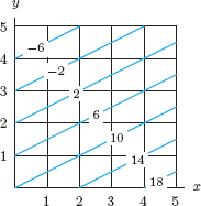
17. You borrow $A at an interest rate of r% (per month) and pay it off over t months by making monthly payments of P = g(A, r, t) dollars. In financial terms, what do the following statements tell you?
(a) g(8000,1, 24) = 376.59
(b) ![]()
(c) ![]()
For Problems 18–20, refer to Table 8.13 on page 395 giving the temperature adjusted for wind chill, C, in °F, as a function f(w, T) of the wind speed, w, in mph, and the temperature, T, in °F. The temperature adjusted for wind chill tells you how cold it feels, as a result of the combination of wind and temperature.
18. Estimate fw(10, 25). What does your answer mean in practical terms?
19. Estimate fT(5, 20). What does your answer mean in practical terms?
20. From Table 8.13 you can see that when the temperature is 20°F, the temperature adjusted for wind-chill drops by an average of about 0.8°F with every 1 mph increase in wind speed from 5 mph to 10 mph. Which partial derivative is this telling you about?
21. In the 1940s the quantity, q, of beer sold each year in Britain was found to depend on I (the aggregate personal income, adjusted for taxes and inflation), p1 (the average price of beer), and p2 (the average price of all other goods and services). Would you expect ∂q/∂I, ∂q/∂p1, ∂q/∂p2 to be positive or negative? Give reasons for your answers.
22. The average price of large cars getting low gas mileage (“gas guzzlers”) is x and the average price of a gallon of gasoline is y. The number, q1, of gas guzzlers bought in a year, depends on both x and y, so q1 = f(x, y). Similarly, if q2 is the number of gallons of gas bought to fill gas guzzlers in a year, then q2 = g(x, y).
(a) What do you expect the signs of ∂q1/∂x and ∂q2/∂y to be? Explain.
(b) What do you expect the signs of ∂q1/∂y and ∂q2/∂x to be? Explain.
23. Figure 8.60 shows the density of the fox population P (in foxes per square kilometer) for southern England. Draw two different graphs of the fox population as a function of kilometers north, with kilometers east fixed at two different values, and draw two different graphs of the fox population as a function of kilometers east, with kilometers north fixed at two different values.

24. Figure 8.60 gives a contour diagram for the number n of foxes per square kilometer in southwestern England. Estimate ∂n/∂x and ∂n/∂y at the points A, B, and C, where x is kilometers east and y is kilometers north.
Find the partial derivatives in Problems 25–30. The variables are restricted to a domain on which the function is defined.
25. fx and fy if f(x, y) = x2 + xy + y2
26. Pa and Pb if P = a2 − 2ab2
27. ![]()
28. ![]()
29. ![]()
30. ![]()
31. A manufacturing company produces two items in quantities q1 and q2, respectively. Total production costs are given by
![]()
Find f(500, 1000), fq1(500, 1000), and fq2 (500, 1000). Give units with your answers and interpret each of your answers in terms of production cost.
32. The Cobb-Douglas production function for a product is given by
![]()
where Q is the quantity produced for a capital investment of K dollars and a labor investment of L.
(a) Find QK and QL.
(b) Find the values of Q, QK and QL given that K = 60 and L = 100.
(c) Interpret each of the values you found in part (b) in terms of production.
33. You are an anthropologist observing a native ritual. Sixteen people arrange themselves with their backs to you along a bench; all but the three on the far left side are seated. The first person on the far left is standing with her hands at her side, the second is standing with his hands raised and the third is standing with her hands at her side. At some unseen signal, the first one sits down, and everyone else copies what his neighbor to the left was doing one second earlier. Every second that passes, this behavior is repeated until all are once again seated.
(a) Draw graphs at several different times showing how the height depends upon the distance along the bench.
(b) Graph the location of the raised hands as a function of time.
(c) What US ritual is most closely related to what you have observed?
34. You are in a stadium doing the wave. This is a ritual in which members of the audience stand up and down in such a way as to create a wave that moves around the stadium. Normally a single wave travels all the way around the stadium, but we assume there is a continuous sequence of waves. Let h(x, t) = 5 + cos(0.5x − t) be the function describing this stadium wave. The value of h(x, t) gives the height (in feet) of the head of the spectator in seat x at time t seconds. Evaluate hx(2, 5) and ht(2, 5) and interpret each in terms of the wave.
35. Find all critical points of f(x, y) = x3 − 3x + y2. Make a table of values to determine if each critical point is a local minimum, a local maximum, a saddle point, or none of these.
36. Find all critical points of f(x, y) = x2 + 3y2 − 4x + 6y + 10.
37. A company sells two products which are partial substitutes for each other, such as coffee and tea. If the price of one product rises, then the demand for the other product rises. The quantities demanded, q1 and q2, are given as a function of the prices, p1 and p2, by
![]()
(a) Write total sales revenue as a function of p1 and p2.
(b) What prices should the company charge in order to maximize the total sales revenue?15
Figure 8.61 shows contours of f. In Problems 38–40 give an approximate maximum or minimum value of f for 0 ≤ x ≤ 300, 0 ≤ y ≤ 300 subject to the given constraint.

38. Minimum, constraint is y = 100
39. Maximum, constraint is y = 100
40. Maximum, constraint is y = x
41. The quantity, Q, of a good produced depends on the quantities x1 and x2 of two raw materials used:
![]()
A unit of x1 costs $127 and a unit of x2 costs $92. We want to minimize the cost, C, of producing 500 units of the good.
(a) What is the objective function?
(b) What is the constraint?
(c) Explain what the Lagrange multiplier, λ = 219, tells us about production.
42. Figure 8.62 shows level curves for production f(x, y) as a function of the quantities x and y of two raw materials utilized. The cost of the materials is 15x + 20y thousand dollars. What is the maximum production possible with a budget of 300 thousand dollars? How much of each raw material should be purchased to achieve this maximum?

43. An automobile manufacturing plant currently employs 1500 workers and has capital investment of 15 million dollars per month. The production function is
![]()
where Q is the number of cars produced per month, x is the number of workers and y is capital investment. Each worker's salary is $5000 per month and each unit of capital costs $4000 per month.
(a) How many cars is the factory currently assembling each month?
(b) Due to the sluggish economy, the factory decides to decrease production to 2000 cars per month. The factory wants to minimize the cost of producing these 2000 cars. How many workers will need to be laid off? By what amount should monthly investment be decreased?
(c) Give the value of the Lagrange multiplier, λ, and interpret it in terms of the car factory.
44. A company manufactures x units of one item and y units of another. The total cost in dollars, C, of producing these two items is approximated by the function
![]()
(a) If the production quota for the total number of items (both types combined) is 39, find the minimum production cost.
(b) Estimate the additional production cost or savings if the production quota is raised to 40 or lowered to 38.
45. A monopolistic producer of two goods A and B has a joint total cost function
![]()
where q1 and q2 denote the quantities of A and B respectively. The demand curves for the corresponding prices p1 and p2 are
![]()
(a) Find the maximum profit if the firm produces a total of 15.
(b) Estimate the new optimal profit if the production quota increases by one unit.
STRENGTHEN YOUR UNDERSTANDING
In Problems 1–60, indicate whether the statement is true or false.
1. If Q = f(x, t) gives the quantity Q of pollutants, in ppm (parts per million), at a distance x kilometers from a waste incinerator at time t hours after incineration ends, we have f(1.5, 6) = 4.1. The units for 1.5 are ppm.
2. If Q = f(x, t) gives the quantity Q of pollutants, in ppm (parts per million), at a distance x kilometers from a waste incinerator at time t hours after incineration ends, we have f(1.5, 6) = 4.1. The units for 6 are hours.
3. If Q = f(x, t) gives the quantity Q of pollutants, in ppm (parts per million), at a distance x kilometers from a waste incinerator at time t hours after incineration ends, we have f(1.5, 6) = 4.1. The units for 4.1 are kilometers.
4. If Q = f(x, t) gives the quantity Q of pollutants, in ppm (parts per million), at a distance x kilometers from a waste incinerator at time t hours after incineration ends, then Q is most likely an increasing function of x.
5. If Q = f(x, t) gives the quantity Q of pollutants, in ppm (parts per million), at a distance x kilometers from a waste incinerator at time t hours after incineration ends, in the statement f(2, 3) = 5, the units of the 2 are km.
6. If f(x, y) is a function of two variables, then f is an increasing function of x if f increases when both x increases and y increases.
7. A function f(x, y) can be both an increasing function of x and a decreasing function of y.
8. The function f(x, y) = x2 − y is a decreasing function of y.
9. If f(x, y) = exy − y2, then the cross-section x = 1 is f(1, y) = ey − 1.
10. If f(x, y) = exy − y2, then the cross-section y = 0 is f(x, 0) = 0.
11. The function f(x, y) = y + 3x − 1 has contours which are lines.
12. The function f(x, y) = x2 − y has contours which are parabolas.
13. For a given function f(x, y) the two contours f(x, y) = 1 and f(x, y) = 2 can never intersect.
14. Contours of the function g(x, y) = 3x + 2y are parallel lines.
15. The function P = 3N1/2V1/2 is a Cobb-Douglas production function.
16. The function P = 10N3V2 is a Cobb-Douglas production function.
17. The function f(x, y) has the same value at all points along a specific contour.
18. A contour can consist of a single point.
19. Contours of a Cobb-Douglas production function are decreasing, concave up.
20. Every point in the domain of g(x, y) has a contour that contains it.
21. The partial derivative fx(a, b) is the rate of change of the function f with respect to x at the point (a, b) with y fixed at b.
22. If P = f(m, t) gives the price P (in dollars) of a used car as a function of its mileage m (in miles) and its age t (in years), then ∂P/∂m has units miles per year.
23. If P = f(m, t) gives the price P (in dollars) of a used car as a function of its mileage m (in miles) and its age t (in years), then ∂P/∂m is most likely to be negative.
24. If W = f(c, t) gives the weight W (in pounds) of a person as a function of their daily food intake c (in calories) and daily aerobic exercise time t (in hours), then ∂W/∂c has units pounds per calorie.
25. If W = f(c, t) gives the weight W (in pounds) of a person as a function of their daily food intake c (in calories) and daily aerobic exercise time t (in hours), then ∂W/∂c is most likely to be negative.
26. If W = f(c, t) gives the weight W (in pounds) of a person as a function of their daily food intake c (in calories) and daily aerobic exercise time t (in hours), then ∂W/∂c and ∂W/∂t most likely have opposite signs.
27. For a function z = f(x, y), assume f(1, 2) = 10 and f(1.1,2) = 10.5 and f(1,2.1) = 10.8 and f(1.1, 2.1) = 11.3. Then fx(1, 2) ≈ 5.
28. For a function z = f(x, y), assume f(1, 2) = 10 and f(1.1, 2) = 10.5 and f(1, 2.1) = 10.8 and f(1.1, 2.1) = 11.3. Then fy (1, 2) ≈ 13.
29. For a function z = f(x, y), assume f(5, 3) = 7 and f(5.1, 3) = 7.9 and f(5, 3.1) = 6.4 and f(5.1, 3.1) = 7.3. Then fx(5, 3) ≈ 9.
30. For a function z = f(x, y), assume f(5, 3) = 7 and f(5.1, 3) = 7.9 and f(5, 3.1) = 6.4 and f(5.1, 3.1) = 7.3. Then fy(5, 3) ≈ 6.
31. If f(x, y) = x2y + 3x then fx(x, y) = 2xy + 3.
32. If f(x, y) = x2y + 3x then fy (1, 2) = 4.
33. If g(u, v) = uev then gu(0, 0) = 1.
34. There exists a function f with fx(x, y) = fy(x, y).
35. The function Q(x, y) = x3y2 is decreasing in the y direction near (1, 2).
36. ![]() .
.
37. For all functions f it is always true that fxx = fyy if fxx and fyy are continuous.
38. If f(x, y) = 3x2e2y then fy(1, 0) < fx(1, 0).
39. ![]() .
.
40. ![]() .
.
41. If f is a function with fx(1, 2) = 0 then (1, 2) is a critical point of f.
42. The point (1, 1) is a critical point of f(x, y) = x2 + y2.
43. The point (3, 2) is a critical point of g(u, v) = (u − 3)2 + (v − 2)2.
44. The function f(x, y) = xey has no critical points.
45. If (0, 0) is a critical point of f then f has either a local maximum or local minimum at (0, 0).
46. If D > 0 and fxx > 0 in the second derivative test at the point (a, b) then f has a local minimum at (a, b).
47. To use the second derivative test on a function f at a point (a, b), we must have fx(a, b) = 0 and fy(a, b) = 0.
48. The function f(x, y) = x2 − y2 has a local minimum at (0, 0).
49. The function f(x, y) = 3xy has a neither a local maximum or minimum at (0, 0).
50. A local minimum of f can also be a global minimum of f.
51. If f has a local maximum at P0 subject to the constraint g(x, y) = c then P0 is a critical point of f.
52. If f has a local maximum at P0 subject to the constraint g(x, y) = c then P0 satisfies the equation g(x, y) = c.
53. If we wish to maximize production given a fixed budget, then the production function is the constraint equation.
54. If we wish to minimize costs given a fixed production level, then the production equation is the constraint equation.
55. The minimum value of f(x, y) = x2 + y2 subject to the constraint x − y = 0 is f(0, 0) = 0.
56. The minimum value of f(x, y) = x2 + y2 subject to the constraint 2x + 3y = 12 is f(0, 0) = 0.
57. If the minimum cost is $50,000 given a fixed production level of 8,000 tons with λ = 120, then we expect production of 8,001 tons to cost about $50,120.
58. If the maximum production level is 50,000 tons given a fixed budget of $80,000 with λ = 120, then we expect production of $50,001 tons to cost about $80,120.
59. The second derivative test can be used to classify a point found by the Lagrange multiplier method as constrained maximum or minimum.
60. If the quantity Q of a good produced depends only on the quantities x and y of two raw materials used to manufacture the good, and there is a total of $50,000 to spend on the two raw materials, then a budget constraint for Q is x + y = 50000.
PROJECTS FOR CHAPTER EIGHT
1. A Heater in a Room
Figure 8.63 shows the contours of the temperature along one wall of a heated room through one winter day, with time indicated as on a 24-hour clock. The room has a heater located at the leftmost corner of the wall and one window in the wall. The heater is controlled by a thermostat about 2 feet from the window.
(a) Where is the window?
(b) When is the window open?
(c) When is the heat on?
(d) Draw graphs of the temperature along the wall of the room at 6 am, at 11 am, at 3 pm (15 hours) and at 5 pm (17 hours).
(e) Draw a graph of the temperature as a function of time at the heater, at the window and midway between them.
(f) The temperature at the window at 5 pm (17 hours) is less than at 11 am. Why do you think this might be?
(g) To what temperature do you think the thermostat is set? How do you know?
(h) Where is the thermostat?

2. Optimizing Relative Prices for Adults and Children
Some items are sold at a discount to senior citizens or children. The reason is that these groups are more sensitive to price, so a discount has greater impact on their purchasing decisions. The seller faces an optimization problem: How large a discount to offer in order to maximize profits? Suppose a theater can sell qc child tickets and qa adult tickets at prices pc and pa, according to the demand functions:
![]()
and has operating costs proportional to the total number of tickets sold. What should be the relative price of children's and adults' tickets?
3. Maximizing Production and Minimizing Cost: “Duality”
A company's production function is P = ![]() for quantities x1 and x2 of two raw materials, costing $4 per unit and $27 per unit, respectively.
for quantities x1 and x2 of two raw materials, costing $4 per unit and $27 per unit, respectively.
(a) How much of each raw material should be used to maximize production if the budget for raw materials is $324? What is the maximum production achieved, P0?
(b) What is the minimum cost at which a production level of P0 can be achieved? How much of each raw material is used at this minimum?
(c) Comment on the relationship between your answers to parts (a) and (b).
FOCUS ON THEORY
DERIVING THE FORMULA FOR A REGRESSION LINE
Suppose we want to find the “best fitting” line for some experimental data. In Appendix A, we use a computer or calculator to find the formula for this line. In this section, we derive this formula.
We decide which line fits the data best by using the following criterion. The data is plotted in the plane. The distance from a line to the data points is measured by adding the squares of the vertical distances from each point to the line. The smaller this sum of squares is, the better the line fits the data. The line with the minimum sum of square distances is called the least-squares line, or the regression line. If the data is nearly linear, the least-squares line will be a good fit; otherwise it may not be. (See Figure 8.64.)

Figure 8.64: Fitting lines to data points
| Example 1 | Find a least-squares line for the following data points: (1, 1), (2, 1), and (3, 3). |
| Solution | Suppose the line has equation y = b + mx. If we find b and m then we have found the line. So, for this problem, b and m are the two variables. We want to minimize the function f(b, m) that gives the sum of the three squared vertical distances from the points to the line in Figure 8.65.
Figure 8.65: The least-squares line minimizes the sum of the squares of these vertical distances The vertical distance from the point (1,1) to the line is the difference in the y-coordinates 1 − (b + m); similarly for the other points. Thus, the sum of squares is
To minimize f we look for critical points. First we differentiate f with respect to b:
Now we differentiate with respect to m:
The equations fb = 0 and fm = 0 give a system of two linear equations in two unknowns:
The solution to this pair of equations is the critical point b = −1/3 and m = 1. Since
we have found a local minimum. This local minimum is also the global minimum of f. Thus, the least-squares line is
As a check, notice that the line y = x passes through the points (1, 1) and (3, 3). It is reasonable that introducing the point (2, 1) moves the y-intercept down from 0 to −1/3. |


Derivation of the Formulas for the Regression Line
We use the method of Example 1 to derive the formulas for the least-squares line y = b + mx generated by data points (x1, y1), (x2, y2), ..., (xn, yn). Notice that we are looking for the slope and y-intercept, so we think of m and b as the variables.
For each data point (xi, yi), the corresponding point directly above the line or below it on the line has the y-coordinate b + mxi. Thus, the squares of the vertical distances from the point to the line is (yi − (b + mxi))2. (See Figure 8.66.)

Figure 8.66: The vertical distance from a point to the line
We find the sum of the n squared distances from points to the line, and think of the sum as a function of m and b:
![]()
To minimize this function, we first find the two partial derivatives, fb and fm. We use the chain rule and the properties of sums.

We now set the partial derivatives equal to zero and solve for m and b. This is easier than it looks: we simplify the appearance of the equations by temporarily substituting other symbols for the sums: write SY for Σyi, SX for Σxi, SXY for Σyixi and SXX for Σ![]() . Remember, the xi and yi are all constants. We get a pair of simultaneous linear equations in m and b; solving for m and b gives us formulas in terms of SX, SY, SXY, and SXX. We separate fb(b, m) into three sums as shown:
. Remember, the xi and yi are all constants. We get a pair of simultaneous linear equations in m and b; solving for m and b gives us formulas in terms of SX, SY, SXY, and SXX. We separate fb(b, m) into three sums as shown:
![]()
Similarly, we can separate fm(b, m) after multiplying through by xi:
![]()
Rewriting the sums as suggested and setting ![]() and
and ![]() equal to zero, we have:
equal to zero, we have:
![]()
Solving this pair of simultaneous equations, we get the result:
![]()
Writing these expressions with summation notation, we arrive at the following result:
The least-squares line for data points (x1, y1), (x2, y2), . . ., (xn, yn) is the line y = b + mx where

| Example 2 | Use these formulas to find the best fitting line for the data point (1, 5), (2,4), (4, 3). |
| Solution | We compute the sums needed in the formulas:
Since n = 3, we have:
and
The least-squares line for these three points is
To check this equation, plot the line and the three points together. |


Many calculators have the formulas for the least-squares line built in, so that when you enter the data, out come the values of b and m. At the same time, you get the correlation coefficient, which measures how close the data points actually come to fitting the least-squares line.
Problems on Deriving the Formula for Regression Lines
In Problems 1–2, use the method of Example 1 to find the least-squares line. Check by graphing the points with the line.
1. (−1, 2), (0, −1), (1, 1)
2. (0, 2), (1, 4), (2, 5)
In Problems 3–5, use the formulas for b and m to check that you get the same result as in the problem or example specified.
3. (−1, 2), (0, −1), (1, 1). See Problem 1.
4. (0, 2), (1, 4), (2, 5). See Problem 2.
5. (1, 1), (2, 1), (3, 3). See Example 1.
In Problems 6–7, we transform nonlinear data so that it looks more linear. For example, suppose the data points (x, y) fit the exponential equation,
![]()
where a and C are constants. Taking the natural log of both sides, we get
![]()
Thus, ln y is a linear function of x. To find a and C, we can use least squares for the graph of ln y against x.
6. The population of the US was about 180 million in 1960, grew to 206 million in 1970, and 226 million in 1980.
(a) Assuming that the population was growing exponentially, use logarithms and the method of least squares to estimate the population in 1990.
(b) According to the national census, the 1990 population was 249 million. What does this say about the assumption of exponential growth?
(c) Predict the population in the year 2010.
7. A biological rule of thumb states that as the area A of an island increases tenfold, the number of animal species, N, living on it doubles. The table contains data for islands in the West Indies. Assume that N is a power function of A.
(a) Use the biological rule of thumb to find
(i) N as a function of A
(ii) ln N as a function of ln A
(b) Using the data given, tabulate ln N against ln A and find the line of best fit. Does your answer agree with the biological rule of thumb?
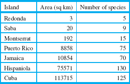
1From Richard G. Lipsey, An Introduction to Positive Economics, 3rd Ed. (London: Weidenfeld and Nicolson, 1971).
2Adapted from S. Beaty and R. Healy, The Future of American Agriculture, Scientific American, Vol. 248, No. 2, February, 1983.
3From the undergraduate senior thesis of Professor Robert Cook, Director of Harvard's Arnold Arboretum.
4Arthur C. Guyton and John E. Hall, Textbook of Medical Physiology, Ninth Edition, p. 288 (Philadelphia: W. B. Saunders, 1996).
5From www.ecolo.org/documents/documents_in_english/WindmillFormula.htm, accessed October 9, 2011.
6Peter G. Welling and Francis L. S. Tse, Pharmacokinetics of Cardiovascular, Central Nervous System, and Antimicrobial Drugs, The Royal Society of Chemistry, 1985, p. 316.
7James E. Gibson, Formaldehyde Toxicity, p. 125 (Hemisphere Publishing Company, McGraw-Hill, 1983).
8From the August 28, 1994, issue of Parade Magazine.
9Adopted from M. Rosser, Basic Mathematics for Economist, p. 316 (New York: Routledge, 1993).
10An explanation of this test can be found, for example, in Multivariable Calculus by W. McCallum et al. (New York: John Wiley, 2009).
11Adapted from M. Rosser, Basic Mathematics for Economists, p. 318 (New York: Routledge, 1993).
12If the constraint has endpoints.
13See W. McCallum et al., Multivariable Calculus (New York: John Wiley, 2009).
14Data from www.nws.noaa.gov/om/windchill, accessed May 30, 2004.
15Adapted from M. Rosser, Basic Mathematics for Economists, p. 318 (New York: Routledge, 1993).