
7
Integrated Vehicle Dynamics Control: Centralized Control Architecture
7.1 Principles of Integrated Vehicle Dynamics Control
Current and future motor vehicles are incorporating increasingly sophisticated chassis control systems to improve vehicle handling, stability, and comfort. These chassis control systems include vehicle stability control (VSC), active suspension system (ASS), electrical power steering (EPS), and active four-wheel steering control (4WS), etc. These control systems are generally designed by different suppliers with different technologies and components to accomplish certain control objectives or functionalities. Especially when equipped into vehicles, control systems often operate independently and thus result in a parallel vehicle control architecture. In such a parallel vehicle control architecture, inevitably there occur interaction and performance conflict among the control systems occur ineviably because the vehicle motions in the vertical, lateral, and longitudinal directions are coupled together in nature. To address the problem, an approach of using an integrated vehicle control system was proposed around the 1990s[1]. An integrated vehicle control system is an advanced system that coordinates all the chassis control systems and components to improve the overall vehicle performance including handling stability, ride comfort, and safety, through creating synergies in the use of sensor information, hardware, and control strategies of different control systems[1,2]. As a result, the application of integrated vehicle control systems brings a number of advantages, including: (1) coordinating the interactions among the different subsystems; (2) further exploiting the potentials of each subsystem through integrating the function of the different subsystems with different work domains; (3) reducing the number of sensors and actuators by sharing and integrating the related ones. As shown in Figure 7.1, a better pareto-optimal solution of the vehicle overall performance is achieved through creating synergies amongst the different subsystems.

Figure 7.1 Principle of an integrated vehicle control system.
A number of control techniques have been designed to achieve the goal of functional integration of the chassis control systems. These control techniques can be classified into three categories according to the extent of function integration of the subsystems, as suggested by Gordon et al.[2] and Yu et al.[3]: (1) decentralized or parallel control; (2) centralized control; and (3) multilayer control. In the decentralized control architecture shown in Figure 7.2, the subsystems of the vehicle are relatively independent and communicate with each other through the onboard network (CAN or LIN) to achieve their local control targets conveniently and flexibly. However, due to the lack of a global control target for the decentralized control architecture, the control architecture can only serve as a combined control structure of the vehicle subsystems at most. Compared to the parallel structure with standalone subsystems, the decentralized control architecture is superior through taking advantage of integrating and sharing the information of sensors and actuators.

Figure 7.2 Decentralized (or Parallel) architecture.
Most of the control techniques used in the previous studies in recent years fall into the second category. Examples include nonlinear predictive control[4], random sub-optimal control[5], robust ![]() [6], sliding mode[7], and artificial neural networks[8]. In the centralized architecture shown in Figure 7.3, a single central controller collects all the vehicle operation information, including information from the sensors and the state estimators, and then generates control commands to the subsystem actuators by applying a global multi-objective optimization algorithm. Therefore, both the advantages and disadvantages are obvious. The centralized architecture has the advantages of controlling and observing all the subsystems in an integrated manner. However, the disadvantages cannot be ignored: the curse of dimensionality caused by the increasing number of subsystems results in tremendous design difficulties. Moreover, the failure of the centralized controller inevitably leads to a total failure of the whole chassis control system. Finally, when the centralized architecture needs to include more required subsystems, the entire centralized architecture has to be redesigned since the architecture lacks flexibility.
[6], sliding mode[7], and artificial neural networks[8]. In the centralized architecture shown in Figure 7.3, a single central controller collects all the vehicle operation information, including information from the sensors and the state estimators, and then generates control commands to the subsystem actuators by applying a global multi-objective optimization algorithm. Therefore, both the advantages and disadvantages are obvious. The centralized architecture has the advantages of controlling and observing all the subsystems in an integrated manner. However, the disadvantages cannot be ignored: the curse of dimensionality caused by the increasing number of subsystems results in tremendous design difficulties. Moreover, the failure of the centralized controller inevitably leads to a total failure of the whole chassis control system. Finally, when the centralized architecture needs to include more required subsystems, the entire centralized architecture has to be redesigned since the architecture lacks flexibility.

Figure 7.3 Centralized architecture.
In contrast, multilayer control has not yet been applied extensively to integrated vehicle control. It is indicated by a relatively small volume of research publications [2,9–14].The multilayer control architecture shown in Figure 7.4 consists of two layers. The upper layer controller monitors the driver’s intentions and the current vehicle state. Based on these input signals, the upper layer controller is designed to coordinate the interactions amongst all the subsystem controllers in order to achieve the desired vehicle state. Thereafter, the control commands are generated by the upper layer controller and distributed to the corresponding individual lower layer controllers. Finally, the individual lower layer controllers execute respectively their local control objectives to control the vehicle dynamics.
In this chapter, the applications of the centralized control architecture are introduced by using various control methods to fulfill the integrated control goal for different subsystems.
Figure 7.4 Multilayer control architecture.
7.2 Integrated Control of Vehicle Stability Control Systems (VSC)
A vehicle stability control system (VSC) is an integrated control system through the function integration of the anti-lock brake system (ABS) and traction control system (TCS) with the active yaw moment control system (AYC). VSC maintains the lateral stability of the vehicle by controlling the longitudinal forces between the tyres and road. As discussed in Section 3.5, the widely-used direct yaw moment control (DYC) method was briefly introduced to achieve the aims of the VSC. To fully explore the work principles of VSC, a control strategy for the sideslip angle of the vehicle center of gravity (CG) is proposed by using dynamic limits of the road surfaces in order to examine the effects on the sideslip angle for different road surfaces. Furthermore, a method for estimating the road adhesion coefficient is proposed by applying both the extended Kalman filter and neural network since estimation of the road adhesion coefficient is an important topic in the area of VSC and is also the basis of designing the control strategy of a VSC[15].
7.2.1 Sideslip Angle Control
As mentioned in Section 3.5 above, the two crucial states to determine the vehicle stability include the yaw rate and sideslip angle. The yaw rate measures the vehicle angular velocity around its vertical inertia axis, and the sideslip angle reflects the deviation of the vehicle on its current driving direction. Therefore, both states must be taken as control targets when designing the VSC.
Moreover, the effects of the sideslip angle resulting from different road surfaces must be taken into consideration. There are two main reasons. First, the stability limit that the vehicle is able to achieve is different for different road surfaces. For example, the stability limit for the road surface with a higher adhesion coefficient is larger than that with a lower adhesion coefficient. Second, the control of the sideslip angle is fulfilled through adjusting the longitudinal forces between the tyres and the road, and the longitudinal forces are directly related to the adhesion coefficient. Therefore, the control strategy for the sideslip angle is proposed by using dynamic limits of road surfaces in order to examine the effects on the sideslip angle for different road surfaces.
7.2.1.1 Development of the Sideslip Angle Control Strategy
7.2.1.1.1 Dynamic Characteristics of the Sideslip Angle
We first investigate the dynamic characteristics of the sideslip angle through performing a simulation study of a 7-DOF vehicle dynamic model. The vehicle is assumed to drive on a road with the adhesion coefficient of 0.3, and the double lane change maneuver is performed. The relationship between the sideslip angle and the sideslip angular velocity is shown in Figure 7.5. In the figure, when the absolute value of the sideslip angle is less than 0.02 rad, the vehicle stays stable; when it is larger than 0.02 rad, the absolute value of the rate of the sideslip angle increases drastically. This phenomenon shows that the vehicle tends to become unstable. Since vehicle stability is directly related to the sideslip motion of the vehicle, this motion must be bounded in order to keep the vehicle stable. Thus, the aim of the sideslip angle controller is to bind the sideslip angle within a suitable region in which the vehicle stays stable. As shown in Figure 7.6, the suitable stability region is defined in the phase plane of the sideslip motion:

Figure 7.5 Simulation results for the relationship between the sideslip angle and sideslip angular velocity.
Figure 7.6 Stability region in the phase plane of the sideslip motion.
The suitable stability region is achieved by selecting suitable values of the parameters C1 and C2. Thus, the sideslip angle controller is proposed in Figure 7.7.

Figure 7.7 Block diagram of the proposed sideslip angle controller.
To demonstrate the effectiveness of the proposed sideslip angle controller, simulation investigations are performed for different driving conditions. First, the driving condition is set as follows: the vehicle is assumed to drive at a constant speed of 120 km/h on a road with a high adhesion coefficient of 0.9, and a double lane change maneuver is performed. As shown in Figures 7.8 and 7.9, the simulation results demonstrate that the sideslip angle is bounded at a relatively small value, and the sideslip motion is stable. In addition, the other driving condition is also performed: in this case, the vehicle speed is set to 60 km/h on a road with a low adhesion coefficient of 0.4, and the double lane change maneuver is also performed. As shown in Figures 7.10 and 7.11, the simulation results demonstrate that the VSC is able to restrain the sideslip at a relatively small value, and hence the sideslip motion stays stable.
Figure 7.8 Response of the sideslip angle.

Figure 7.9 Phase plane of the sideslip motion.

Figure 7.10 Response of the sideslip angle.

Figure 7.11 Phase plane of the sideslip motion.
However, as shown in Figure 7.10, the peak value of the sideslip angle is quite large and the phenomenon contradicts reality since the vehicle cannot stay stable with such a large sideslip angle. The simulation results show that it is inappropriate to define directly the handling limit as the control objectives since the lateral tyre force has already been close or even beyond the saturation point when the vehicle approaches the handling limit.
Therefore, an effective control method must determine the control objectives to generate the corrective yaw moment to pull the vehicle back to the stable region before it approaches the handling limit. The definitions of the reference region and the control region for designing the sideslip angle controller are illustrated in Figure 7.12. There are two boundaries, the inner boundary and outer boundary, which define the reference region and the control region, respectively. When the vehicle state lies inside the reference region, the vehicle is considered to be stable and no control action is required. When the vehicle state reaches the control region, which is bounded by the inner boundary and the outer boundary, the VSC is actuated and thus the corrective yaw moment is generated by the sideslip angle controller to pull the vehicle back into the reference region.

Figure 7.12 Definition of the reference region and control region.
As discussed earlier in Section 7.2.1, the effects of the sideslip angle resulting from different road surfaces must be taken into consideration. Thus the determination of the above-mentioned two boundaries must also consider the effects of the road adhesion coefficients. As shown in Figure 7.13, the outer boundary is defined as a specific value of the sideslip angle when the lateral tyre force reaches the saturation point, while the inner boundary is defined as a specific value of the sideslip angle when the lateral tyre force reaches the linear limit.

Figure 7.13 Definition of the two boundaries for designing the sideslip angle controller.
7.2.1.1.2 Outer Boundary of the Sideslip Angle
To determine the outer boundary of the sideslip angle, a dynamic boundary is constructed by considering the effects of the road adhesion coefficients. The lateral acceleration of the C.G. is given as:
Considering the sideslip angle as relatively small, we have ![]() . Therefore, the above equation can be rewritten as:
. Therefore, the above equation can be rewritten as:

Since ![]() , and the latter two terms in equation (7.3) are relatively small compared to the first term, the upper limit of the yaw rate r is selected as:
, and the latter two terms in equation (7.3) are relatively small compared to the first term, the upper limit of the yaw rate r is selected as:
Accordingly, the upper limit of the sideslip angle is chosen as:
According to the above equation, when the road adhesion coefficient ![]() , the sideslip angle equals to 0.17 rad; when
, the sideslip angle equals to 0.17 rad; when ![]() , the value is 0.08 rad. The above equation can be adjusted according to different vehicle physical parameters.
, the value is 0.08 rad. The above equation can be adjusted according to different vehicle physical parameters.
7.2.1.1.3 Inner Boundary of the Sideslip Angle
When the vehicle state lies inside the linear region, the yaw rate r is derived from the 2-DOF linear vehicle dynamic model:

where  . When
 ![]() , the above equation is given as follows:
, the above equation is given as follows:
The above equation shows that the steady state gain of the yaw rate is linear with the steering angle of the front wheel when the vehicle lies inside the linear region. Therefore, it is possible to determine whether the vehicle lies inside the linear region by examining whether the above linear relationship exists. A simulation study is performed to demonstrate the relationship of the two variables. As shown in Figures 7.14 and 7.15, the simulation results illustrate that the yaw rate r is linear with the steering angle of the front wheel δf when δf is smaller than 0.05 rad. However, with the increase on the steering angle δf, the relationship tends to be nonlinear.

Figure 7.14 Relationship between the steady state gain of the yaw rate and the steering angle of the front wheel.
Figure 7.15 Steering angle of the front wheel.
As a matter of fact, only an approximately linear relationship exists for the yaw rate r and the steering angle of the front wheel δf since most vehicles have understeer characteristics. The relationships for the cases of understeer and neutral steer are illustrated in Figure 7.16. Therefore, a weighting function is constructed as follows to compensate for the nonlinear relationship
The weighting function is illustrated in Figure 7.17.

Figure 7.16 Relationships between r and δf. for the cases of understeer and neutral steer.

Figure 7.17 Weighting parameter for the yaw rate.
7.2.1.2 Sideslip Angle Controller Design
The nonlinear sliding mode control method is applied to the design of the sideslip angle controller since the controller is actuated mainly in the nonlinear region[16]. The state space equation of the 2-DOF vehicle dynamic model is derived as follows, with the assumptions of a constant forward speed and a small sideslip angle:
where  ,
,
A system with the same order is selected as the ideal model:

where ΔM is the corrective yaw moment generated by the controller; ![]() is the state of the ideal model;
is the state of the ideal model; ![]() is the input for the bounded model;
is the input for the bounded model; ![]() is the output of the model; (A, B) and (Am, Bm) is controllable, respectively; and (Am, Cm) is observable. Let the sliding hyper plane be:
is the output of the model; (A, B) and (Am, Bm) is controllable, respectively; and (Am, Cm) is observable. Let the sliding hyper plane be:
Decomposing the input matrix B as:

and ![]() , we obtain:
, we obtain:
where  , and
, and ![]() . Thus,
. Thus,

where ![]() and
and ![]() . Substituting equation (7.13) into equations (7.10) and (7.11), we have:
. Substituting equation (7.13) into equations (7.10) and (7.11), we have:

where,

The expression for the canonical system is derived as:

Through the following transformation of coordinates:

i.e.
Equation (7.16) becomes:

When the system reaches the switch plane, we obtain:

Substituting equation (7.19) into equation (7.18),
where ![]() , and K can be determined by pole assignment. And hence, the hyper plane matrix of the system is expressed as:
, and K can be determined by pole assignment. And hence, the hyper plane matrix of the system is expressed as:
Assuming ![]() , the state error and its derivative are defined as:
, the state error and its derivative are defined as:
The sliding mode function for the error space is defined as:
Its derivative is given as:
When the matrices S and B are invertible, the equivalent control law is given as:
Substituting equation (7.26) into equation (7.23),
Let ![]() ,
, ![]() , and
, and ![]() . The above system error equation (7.27) can be rewritten as:
. The above system error equation (7.27) can be rewritten as:
And the error equation (7.23) can be expressed as:
Defining the following transformation for the error e,
Let ![]() and
and ![]() . Combining equation (7.29) and equation (7.30), the switch hyper plane of the error is given as:
. Combining equation (7.29) and equation (7.30), the switch hyper plane of the error is given as:
Defining the control input for the system as
To make the system converge on to the sliding surface, the following condition must be satisfied:
where ![]() , only considering the continuous term of ΔM, we have:
, only considering the continuous term of ΔM, we have:

Substituting the above equation into equation (7.33), the constraint condition is derived as follows:

7.2.1.3 Simulation Study
To demonstrate the effectiveness of the proposed sideslip angle controller, simulation investigations are performed for different driving conditions. First, the driving condition is set as follows: the vehicle is assumed to drive at a constant speed of 60km/h and 120km/h, respectively. The road adhesion coefficient is selected as 0.4 and 0.9, respectively. The double lane change maneuver is performed. For comparison, the commonly-used controller with a static boundary is also applied. The simulation results for the adhesion coefficient of 0.9 and 0.4 are illustrated in Figures 7.18–7.20, and Figures 7.21–7.23, respectively. As shown in Table 7.1, a quantitative analysis of the simulation results is also performed to better demonstrate the simulation results.
Table 7.1 Comparison of the simulation results.
| Adhesion coefficient | Control objective | Maximum | ||
| Controller with static boundary | Controller with dynamic boundary | Improvement | ||
| 0.9 | Yaw rate | 0.52 | 0.43 | 17% |
| Sideslip angle | 0.095 | 0.061 | 36% | |
| 0.4 | Yaw rate | 0.34 | 0.32 | 6% |
| Sideslip angle | 0.079 | 0.046 | 42% | |

Figure 7.18 Yaw rate.


Figure 7.20 Phase plane of the sideslip motion.

Figure 7.21 Yaw rate.


Figure 7.23 Phase plane of the sideslip motion.
It can be observed from the simulation results that the proposed sideslip angle controller is able to bound the sideslip angle at a relatively small value, and hence the lateral stability of the vehicle is achieved for both the roads with the high adhesion coefficient and low adhesion coefficient. However, the commonly-used controller with the static boundary only performs well on the road with a high adhesion coefficient. As shown in Figure 7.23, the vehicle cannot stay stable on the road with a low adhesion coefficient.
7.2.2 Estimation of the Road Adhesion Coefficient
Estimation of road adhesion coefficient is crucial in developing VSC since it is the basis for implementing the VSC. There are two main reasons: first, an effective control strategy of VSC must consider the effects of the road adhesion coefficients on the stability limits. Second, VSC must be able to precisely adjust the tyre force to execute the control commands. Adjusting the tyre force depends mainly on whether or not the road adhesion coefficient is able to be estimated precisely.
A large number of estimation methods have been developed through the brake driving condition. During the process of braking, the relationship between the road adhesion coefficient and brake efficiency factor is constructed, and thus the road adhesion coefficient is calculated[17, 18]. However, there is no severe braking when the VSC intervenes since the VSC works mainly under the steer driving condition. Therefore, it is necessary to develop methods to estimate the road adhesion coefficient for the VSC under the steer driving condition. As discussed earlier, with the increase of the sideslip angle, the lateral tyre force increases from the linear region to the nonlinear region and is close to or even beyond the saturation point. In addition, the inner boundaries of the sideslip angle are different with respect to the different road adhesion coefficients[19, 20]. Therefore, the method for estimating the road adhesion coefficient is developed through determining precisely the point that the vehicle reaches the nonlinear region, and thus calculating the corresponding sideslip angle.
However, if the lateral tyre force does not have a distinct transformation from the linear region to the nonlinear region when the change of the steering angle is quite small, it is necessary to take this case into account when developing the estimation methods. Figure 7.24 shows the simulation results of the sideslip angles for a road adhesion coefficient of 0.4 and 0.9, respectively, when the same yaw rate illustrated in Figure 7.25 is maintained. The simulation results demonstrate that the sideslip angle for the low road adhesion coefficient is larger than that for the high road adhesion coefficient when the yaw rate stays the same. The reason is that the sideslip angle must increase for the low road adhesion coefficient in order to provide the same lateral tyre force. Therefore, this characteristic is applied to design the estimation method when the change of the steering angle is quite small.

Figure 7.24 Sideslip angle for different road adhesion coefficient.

Figure 7.25 Yaw rate.
Moreover, as illustrated in Figure 7.26, it is observed that the vertical load has a great effect on the sideslip angle and the lateral tyre force. In this case, it may not be precise enough to estimate the road adhesion coefficient by using only one sideslip angle out of the four wheels. Therefore, the estimation method is proposed to use the sideslip angles of the two front wheels since the sideslip angles of the two rear wheels are relatively small.

Figure 7.26 Effects of vertical load on the wheel sideslip characteristics.
7.2.2.1 Estimation of the Sideslip Angle
As discussed above, the estimation of the sideslip angle is important for the estimation of the road adhesion coefficient. thus, the accuracy of the estimation of the road adhesion coefficient is mainly determined by the accuracy of the sideslip angle. To achieve this aim, an extended Kalman filter is used to accurately estimate the vehicle velocity vx and vy, and then the sideslip angle is calculated according to the wheel model. For the Kalman filter developed in this section, the vehicle velocity, which is calculated from the 2-DOF vehicle dynamic model, is used as the estimated value, while the acceleration calculated from the 7-DOF vehicle model is used for calculating the measured value. Thus, the Kalman filter is derived as:
where  ;ax and ay are the longitudinal and lateral acceleration, respectively; T is the period of sampling cycle; vxa and vya are the longitudinal and lateral vehicle velocity calculated from the 2-DOF vehicle dynamic model, respectively; k is the number of iterations; ε and ω are the measured error and prediction error of the system model. It is assumed that they are independent of each other and subject to the Gaussian distribution, and their covariances are denoted as R and Q. Therefore, the expanded Kalman filter proceeds in two steps. In the first step, the sampling value and error increment between the two samplings are calculated according to equation (7.38) and equation (7.39).
where ![]() is the prediction value;
is the prediction value; ![]() is the covariance of the prediction error; and
is the covariance of the prediction error; and  is the dynamic matrix obtained by the linearized system state equation when calculating
 ![]() . For the second step, the measured value is amended according to the system prediction value and prediction error during the sampling, as expressed in equations (7.40)–(7.42).
. For the second step, the measured value is amended according to the system prediction value and prediction error during the sampling, as expressed in equations (7.40)–(7.42).
where  is the matrix obtained by the linearized system output equation in the prediction process.
7.2.2.2 Proposed Estimation Method of the Road Adhesion Coefficient
The block diagram of the estimation method of the road adhesion coefficient is shown in Figure 7.27. First, the vehicle longitudinal and lateral velocity is calculated by the expanded Kalman filter according to the outputs of the 7-DOF vehicle dynamic model and the 2-DOF vehicle dynamic model. Then, the parameters required for the road estimation method are calculated from the 7-DOF vehicle dynamic model, including the yaw rate gain, front steering angle, and yaw rate. Finally, the adhesion coefficient is estimated by the trained neural network. Obviously, the whole estimation process is an open loop system.

Figure 7.27 Block diagram of the road estimation method.
The linear boundary limitation shown in Section 7.2.1 introduces the approach to determine if the vehicle is under a nonlinear state according to the yaw rate gain. However, the yaw rate gain is a fixed value, and hence it is not accurate enough to determine the vehicle state according to the r/δf threshold. To overcome this difficulty, the error Back Propagation (BP) neural network[21–25] is adopted since it is effective in handling nonlinear problems because of the learning ability of the neural network algorithm. Moreover, the genetic algorithm optimization method is applied to the BP neural network. Therefore, the accuracy of determination of the vehicle state can be improved significantly through heavy learning on some typical test results.
The BP neural network uses a three-layer feed forward structure as illustrated in Figure 7.28. There are four nodes on the input layer, including the yaw rate gain r/δf, side slip angles of the two front wheels αfl, αfr, and yaw rate r; one output node on the output layer, i.e., the road adhesion coefficient; the nodes on implicit layer are determined by the test results during the learning process.

Figure 7.28 Three-layer BP neural network structure.
A genetic algorithm is used to optimize the weighting parameters of each node in the neural network. E is defined as the overall training error of the network
where ![]() is a set of chromosome; s is the summation of the number of the weighting parameters and the number of the thresholds of all the nodes; wi is the i-th connection weighting parameter of the network; M is the total number of the connection weighting parameters; θK is the threshold of the K-th neuron; and K is the total number of neurons on the implicit and output layers. In addition, the following weighting parameters must be determined in the neural network: the connection weighting parameters wik between the nodes on the input and implicit layer, and the connection weighting parameters wkp between the nodes on the implicit and output layer; θK is the threshold of the neuron on the implicit layer; and θp is the threshold of the neuron on the output layer. The following steps of the optimization process are performed:
is a set of chromosome; s is the summation of the number of the weighting parameters and the number of the thresholds of all the nodes; wi is the i-th connection weighting parameter of the network; M is the total number of the connection weighting parameters; θK is the threshold of the K-th neuron; and K is the total number of neurons on the implicit and output layers. In addition, the following weighting parameters must be determined in the neural network: the connection weighting parameters wik between the nodes on the input and implicit layer, and the connection weighting parameters wkp between the nodes on the implicit and output layer; θK is the threshold of the neuron on the implicit layer; and θp is the threshold of the neuron on the output layer. The following steps of the optimization process are performed:
- Code the network connection weighting parameters by real numbers.
- Generate randomly an initial population using the small cluster generation method.
- Evaluate the performance of the individuals according to a fitness function. The fitness function f(x) is defined as the reciprocal of the error, i.e.,
 .
. - Obtain the initial network connection weighting parameters by decoding every individual. Then, the overall error is calculated by inputting the initial network connection weighting parameters and the samples.
- Select, crossover, and mutate the parent population and produce the next generation of population.
- Calculate the fitness value of each individual in the current generation and sort them in an ascending order.
- Obtain the optimal initial weighting parameters of the BP network by decoding the optimal individual. Then calculate the overall error E after adjusting the weighting parameters.
- If the overall error E is less than the assigned target value, the training is terminated. Otherwise, the weighting parameters obtained from the current optimization process is used as the initial weighting parameter of the next training, and step (5) is repeated.
The training sample of the proposed BP neural network is selected from the VSC test results performed on a test vehicle[15]. The adhesion coefficient of the test road is approximately 0.8. Figures 7.29–7.32 show the measured steering angle at the wheel and the yaw rate under the maneuver of step steering and double lane change. The side slip angles of the two front wheels can be calculated by the test results.

Figure 7.29 Steering angle of the front wheel under the maneuver of step steering.


Figure 7.31 Steering angle of the front wheel under the maneuver of double lane change.

Figure 7.32 Yaw rate under the maneuver of double lane change.
7.2.2.4 Simulation Investigation
To demonstrate the performance of the proposed estimation method of the road adhesion coefficient a simulation investigation is performed by selecting the road adhesion coefficient as 0.9 and 0.4, respectively, and the vehicle speed is set as 60 km/h. A sinusoidal input is given as the steering angle. The simulation model is constructed in Simulink as shown in Figure 7.33, and the simulation results are illustrated in Figures 7.34 and 7.35.

Figure 7.33 Simulation model in Simulink.

Figure 7.34 Estimation of a high road adhesion coefficient of 0.9.

Figure 7.35 Estimation of a low road adhesion coefficient of 0.4.
It can be seen from Figures 7.34 and 7.35, and Table 7.2 that the proposed estimation method is able to estimate accurately the road adhesion coefficient for both high and low adhesion coefficients, with an acceptable error. In addition, it can be observed that there are small undulations in the simulation results since the proposed estimation method is open loop; hence, it lacks feedback and self-adjusting mechanisms to compensate for the estimation results.
Table 7.2 Estimation results for high and low adhesion coefficients.
| Adhesion coefficient | Mean value | Error |
| 0.9 | 0.87 | 3.3% |
| 0.4 | 0.41 | 2.5% |
7.3 Integrated Control of Active Suspension System (ASS) and Vehicle Stability Control System (VSC) using Decoupling Control Method
Vehicle Stability Control (VSC) system generates a proper yaw moment on the vehicle through the tyre braking or driving forces, and hence improve the vehicle performance in both the lateral and yaw motions. In addition, the active suspension system (ASS) is able to control the vehicle attitude and regulate the vehicle vertical load transfer during pitch and roll motions by adjusting the suspension stiffness and damping characteristics. Therefore, the main purpose of integrating the VSC with the ASS is to improve the overall vehicle performance, including the lateral stability and ride comfort, through the coordinated control of the VSC and ASS system, especially under critical driving conditions.
7.3.1 Vehicle Dynamic Model
To develop the integrated control of VSC and ASS, the 7-DOF dynamic model is established by considering the interactions between the VSC and ASS, which is analyzed in Chapter 6. The dynamic model shown in Figure 7.36 includes both the VSC and ASS, and the equations of motion can be derived as follows.

Figure 7.36 7-DOF Vehicle dynamic model. (a) Longitudinal and lateral motion. (b) Pitch motion.
Lateral motion
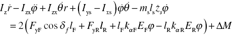
Yaw motion
Vertical motion
where
Roll motion

Pitch motion
where m, ms, and mu are the vehicle mass, sprung mass, and unsprung mass, respectively; xc, yc, and zc are the Cartesian coordinates of the vehicle center of gravity; xs, ys, and zs are the Cartesian coordinates of the center of gravity of the sprung mass; uc is the vehicle longitudinal speed; ϕ and θ are the pitch and roll angles, respectively ; r is the yaw rate of the vehicle; δf is the steering angle of the front wheel; FYF and FYR are the front and rear lateral tyre forces, respectively; EF and ER are the roll camber coefficients of the front and rear wheels, respectively; kαF and kαR are the cornering stiffness of the front and rear tyres, respectively; h is the height of the vehicle center of gravity; hs is the vertical distance between the centers of gravity of both the vehicle and the sprung mass; Iz is the moment of inertia of the vehicle mass about axis zc; Izx is the product of inertia of the vehicle mass about axis xc and zc; Ixu is the moment of inertia of the sprung mass about axis xc; Ixs, Iys, and Izs are the moments of inertia of the sprung mass about axis xs, ys, zs, respectively; Ixzu is the product of inertia of the sprung mass about axis xc and zc; Izxs is the product of inertia of the sprung mass about axis xs and zs; ΔM is the vehicle corrective yaw moment generated by VSC; ls is the longitudinal distance between the centers of gravity of the vehicle mass and sprung mass; lF and lR are the longitudinal distances between the vehicle center of gravity and the front and rear axles, respectively; fFL, fFR, fRL, and fRR are the front-left, front-right, front-left, and rear-left, and rear-right control forces of the active suspension, respectively; zui is the vertical displacement of the i-th unsprung mass; csi is the damping coefficient of the i-th damper; ksi is the suspension stiffness of the i-th suspension; dF and dR are the half of front and rear wheel track, respectively.
7.3.2 2-DOF Reference Model
The 2-DOF vehicle linear dynamic model is adopted as the vehicle reference model to generate the desired vehicle states in this study since the 2-DOF model reflects the desired relationship between the driver’s steering input and the vehicle yaw rate. The equations of motion are expressed as follows by assuming a small sideslip angle and a constant forward speed.


7.3.3 Lateral Force Model
To simplify the design of the integrated control system, a small sideslip angle is assumed and hence the tyre displacement is linear. Therefore, the front and rear lateral forces are derived by considering the vehicle roll steering effect:


where GF and GR are the roll steering coefficients of the front and rear axles, respectively.
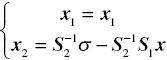
7.3.4 Integrated System Control Model
The state variables are defined as follows for the integrated VSC and ASS control system, by combining equations (7.44)–(7.49), and equations (7.52) and (7.53).
In addition, the variables of the external disturbance for the integrated control system are defined as:
where z0i is the stochastic excitation of each tyre generated by the road unevenness; and δf is the steering angle of the front wheel generated by the driver. As mentioned earlier in this chapter, the VSC system generates an additional yaw moment to track the desired vehicle states, and the ASS adjusts the suspension stiffness and damping characteristics to improve the vehicle ride comfort, and also indirectly improves the handling stability through regulating the load transfer. Therefore, the control input variables for the integrated control system are defined as:
The goal of the integrated VSC and ASS control system is to improve the vehicle handling stability and ride comfort. Therefore, the output variables of the integrated control system include the vehicle yaw rate r, the sideslip angle β, the vertical acceleration at the vehicle center of gravity ![]() , the suspension deflection fd, and the vehicle roll angle ϕ, by considering the measurability of these signals,
, the suspension deflection fd, and the vehicle roll angle ϕ, by considering the measurability of these signals,
The state equation and the output equation are then obtained as:

where A, C are the 16 × 16 input matrix and the 5 × 16 output matrix, respectively; B1, B2 are the 16 × 1 input matrices; D is the 16 × 1 direct transfer matrix; f(x, t) is the coupling term of the state variable with size of 16 × 1.
It is clear that the VSC/ASS integrated control system defined in equation (7.58) is a typical multivariable nonlinear system. Due to the correlations between the tyre longitudinal and vertical forces, and also the interactions among the roll, pitch, and lateral motions, the VSC and ASS are highly coupled. The coupling effects, i.e., a certain control input affecting multiple outputs, are caused by the coupling correlation term included in the state variable. Therefore, it is required to decouple the above-mentioned five control loops and hence achieve that a certain output is controlled solely by one control input in order to improve the overall vehicle performance.
7.3.5 Design of the Decoupling Control System
The decoupling method of nonlinear system is applied to the integrated VSC and ASS system established in equation (7.58) to derive the state feedback control law[26].
7.3.6 Calculation of the Relative Degree
According to the decoupling theory of nonlinear system, the calculation of the relative degree of the original integrated control system is required in order to apply the state feedback control and transform the original nonlinear coupled system into the independent decoupled subsystems. The calculation process is described as follows: first, the derivatives of the control output y are computed with respect to time. Various orders of the derivatives continue to be computed until the input variable u is included explicitly in the output derivative function. Thus, the corresponding derivative order is the system relative degree. In addition, the rank of the Jacobian matrix can be determined through the Interactor algorithm of nonlinear systems[27]. The detailed calculation of the relative degree is demonstrated below.
- Perform the derivative of the control output variable y1 with order
 :
:

Let
 , then
  , and
, and  .
. - Perform the derivative of the system output variable y2 with order
 :
:

Since the control input u is not included explicitly in
 , the derivative of the system output y2 with order
  is then computed:
Let
 ,
,  , then
  .
. - For the integrated system output variable
 , it can be seen that the control input variables fFL, fFR, fRL, and fRR are included in y3, then
  .
.

Let
 , then
  , and
, and  .
. - Similarly, the derivatives of the system outputs y4 and y5 are performed. We obtain
 and
and  ; and the system Jacobian matrices
  and
and  are full ranked, i.e., the ranks are 4 and 5, respectively.
Therefore, the relative degree of the original integrated control system is
 according to the definition of the relative degree.
7.3.7 Design of the Input/Output Decoupling Controller
For the multivariable coupled integrated system, the purpose of the decoupling controller is to make a certain control input ![]() rely solely on the system state variable x and some other independent reference variables
rely solely on the system state variable x and some other independent reference variables ![]() through developing the state feedback law. Thus, the system control input satisfies the following relationship:
through developing the state feedback law. Thus, the system control input satisfies the following relationship:
When the state feedback law defined in equation (7.59) is applied on the coupled integrated system, the i-th component of the closed loop system output yi is affected solely by the i-th reference variable vi, and therefore the decoupling of the control channels of the close loop system is achieved.
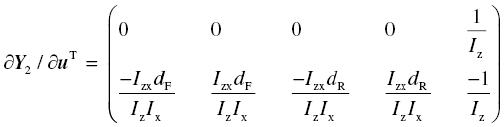
According to the nonlinear decoupling control theory, the relative degree ![]() of the integrated control system is obtained by computation, and also the system Falb-Wolovich matrix (i.e., decoupling matrix) E(x) at the equilibrium point is given as:
of the integrated control system is obtained by computation, and also the system Falb-Wolovich matrix (i.e., decoupling matrix) E(x) at the equilibrium point is given as:

And the system matrix b(x) is obtained as:
Therefore, the state feedback is defined as:

When the state feedback control law u1(x) is applied to the coupled integrated control system, the coupled integrated system is transformed into a decoupled system with independent control channels. The state feedback control law is represented as:
7.3.8 Design of the Disturbance Decoupling Controller
The purpose of the system disturbance decoupling is to fulfill the independence between the control output y in the close loop system and the external disturbance w through designing an appropriate state feedback law. For the integrated control system, the state feedback control law is constructed as follows by assuming that the system external disturbance is measurable.
Therefore the state feedback control law of the coupled integrated system is designed by combining the developed input/output decoupling controller given in equation (7.63) and the disturbance decoupling controller given in equation (7.64).
7.3.9 Design of the Closed Loop Controller
The decoupled integrated system not only eliminates the coupling effects between the control channels, but reduces the influence of the external disturbance on the system control output variable. However, the independent reference variable v in the proposed state feedback control law is unable to improve the control performance of the integrated system since a corrective action is not applied to the independent reference variable. To overcome the problem, a composite controller is proposed through integrating the close loop controller and the decoupling controller in order to improve the overall quality of the system response. As illustrated in Figure 7.37, the proposed integrated control system is decoupled into five independent single-variable systems, and then the closed loop controller is applied to effectively control the decoupled integrated control system.
Figure 7.37 Block diagram of the integrated control system.
7.3.10 Design of the ASS Controller
A PID controller is applied to improve the control performance of the closed loop ASS. By considering the ASS control target, the inputs of the PID controller are selected to include the differences e between the desired and the actual values of the vertical acceleration of the vehicle center of gravity, the suspension deflection, and the roll angle, which are given as:
Therefore, the PID control law is constructed as:

7.3.11 Design of the VSC Controller
A fuzzy control strategy is used for the design of the VSC system, and the block diagram of the proposed VSC control system is shown in Figure 7.38. In the VSC fuzzy control system, the yaw rate and the sideslip angle are selected as the control objectives. As shown in the figure, the VSC fuzzy control system has two input variables, the tracking errors e1 and e2, and the differences of the errors ec1 and ec2 for the yaw rate and the sideslip angle, respectively. The output variables are defined as the corrective yaw moments ΔM1 and ΔM2. Thus, the overall corrective yaw moment is defined as a linear combination of the two:
where n is the weighting coefficient.

Figure 7.38 Block diagram of the fuzzy control system for the VSC.
To determine the fuzzy controller output for the given error and its difference, the decision matrix of the linguistic control rules is designed and presented in Tables 7.3 and 7.4, respectively. In the tables, seven fuzzy sets are used to represent the states of the inputs and outputs, i.e., {PB,PM,PS,ZE,NS,NM,NB}. A trigonometric function is adopted as the basic membership function, and a trapezoidal function is used for the fuzzy boundary. In addition, the dividing density is relatively higher around the zero value (ZE) of the membership function of the fuzzy input, while it is relatively smaller at a distance from the ZE value, in order to improve the control sensitivity. These rules are determined based on expert knowledge and a large number of simulation results performed in the study. Finally, the outputs of the fuzzy controllers ΔM1 and ΔM2 are defuzzified by applying the centroid method to the fuzzy output.
Table 7.3 Fuzzy rule bases for yaw rate.
| ΔM1 | ec1 | |||||||
| NB | NM | NS | ZE | PS | PM | PB | ||
| e1 | NB | PB | PB | PB | PB | PM | ZE | ZE |
| NM | PB | PB | PB | PB | PM | ZE | ZE | |
| NS | PM | PM | PM | PM | ZE | NS | NS | |
| ZE | PM | PM | PS | ZE | NS | NM | NM | |
| PS | PS | PS | ZE | NM | NM | NM | NM | |
| PM | ZE | ZE | NM | NB | NB | NB | NB | |
| PB | ZE | ZE | NM | NM | NB | NB | NB | |
Table 7.4 Fuzzy rule bases for the sideslip angle.
| ΔM2 | ec2 | |||||||
| NB | NM | NS | ZE | PS | PM | PB | ||
| e2 | NB | PB | PB | PM | PM | PS | ZE | ZE |
| NM | PB | PB | PM | PM | PS | ZE | ZE | |
| NS | PB | PB | PM | PM | PS | ZE | NM | |
| ZE | PB | PM | PM | ZE | NM | NM | NB | |
| PS | PM | PM | ZE | NS | NM | NM | NB | |
| PM | ZE | ZE | NS | NS | NM | NM | NB | |
| PB | ZE | ZE | NS | NM | NM | NM | NB | |
7.3.12 Simulation Investigation
In order to evaluate the performance of the developed integrated control system, i.e., the centralized control system using decoupling control method, a simulation investigation is performed. The performance and dynamic characteristics of the integrated control system are analyzed using MATLAB/Simulink. The road excitation is set as the filtered white noise expressed in equation (7.58). After tuning the parameter setting for the integrated control system, we select ![]() ,
, ![]() , and
, and ![]() for the closed loop ASS controller; the weighting coefficient
for the closed loop ASS controller; the weighting coefficient ![]() in the VSC system fuzzy controller. The vehicle physical parameters are presented in Table 7.5. The centralized control using decoupling control method control and the decentralized control (i.e., the VSC and ASS subsystem controllers work independently) are compared to demonstrate the performance of the integrated control system. Three driving conditions are performed, including step steering input, single lane change, and double lane change. The following discussions are made by comparing the centralized control system with the decentralized control system on the corresponding performance indices.
in the VSC system fuzzy controller. The vehicle physical parameters are presented in Table 7.5. The centralized control using decoupling control method control and the decentralized control (i.e., the VSC and ASS subsystem controllers work independently) are compared to demonstrate the performance of the integrated control system. Three driving conditions are performed, including step steering input, single lane change, and double lane change. The following discussions are made by comparing the centralized control system with the decentralized control system on the corresponding performance indices.
Table 7.5 Vehicle physical parameters.
| Symbol (unit) | Value |
| m(kg) | 3018 |
| ms(kg) | 2685 |
| mui(kg) | 333/4 |
| r0(m) | 0.4 |
| h(m) | 0.938 |
| hs(m) | 0.1 |
| H(m) | 0.838 |
| dF /dR(m) | 0.8/0.9 |
| lF /lR(m) | 1.84/1.88 |
| ls(m) | 0.15 |
| kti(i=1,2, 3,4)(N/m) | 420000(1,2)/350000(3,4) |
| ksi(i=1, 2, 3,4)(N/m) | 44444(1,2)/35000(3,4) |
| csi(i=1,2,3,4) (N.s/m) | 1200(1,2)/900(3,4) |
| k∞F /k∞R (N/rad) | 29890/50960 |
| Iz(kg.m2) | 10437 |
| Izx(kg.m2) | 2030 |
| Ijs(j=x,y,z) (kg.m2) | 1744/3000/9285 |
| Ixu(kg.m2) | 1996 |
| Ixzu(kg.m2) | 377.8 |
| Gf/Gr | 0.114/0.1 |
| Ef/Er | 0.8/0.6 |
| Jp(kg.m2) | 0.06 |
| ks(N.m/rad) | 90 |
| Bp(N.m.s/rad) | 0.3 |
| d(m) | 0.1 |
| G(dimensionless) | 20 |
| G0(m3/cycle) | 5.0×10⁻⁶ |
- (1) Step steering input maneuver
The simulation is conducted according to GB/T6323.2-94 controllability and stability test procedure for automobiles – steering transient response test (steering wheel angle step input). The step steering input to the wheel is set as 1.57 rad and the vehicle drives around a circle at a constant speed of 60 km/h. The road adhesion coefficient is selected as 0.6. The simulation results are shown in Figure 7.39.
It is clearly shown in Figure 7.39(a)–(c) that the peak value of the vehicle vertical acceleration for the centralized control is reduced by 30.6% from 2.48 m. s– 2 to 1.72 m. s– 2, the peak value of the roll angle is reduced by 8.1% from 0.099 rad to 0.091 rad, and the peak value of the suspension deflection is reduced by 14.6% from 0.048m to 0.041 m, compared with those for the decentralized control. The results indicate that the centralized integrated control system is able to decrease the influence from the external disturbance on the system control output through applying the disturbance decoupling controller since the road excitation has the major effect on the vehicle ride comfort.
It is observed that in Figure 7.39(d) and (e) that the overshoots of the yaw rate and sideslip angle for the centralized control are reduced by 13.1% and 7.2%, respectively, compared with those for the decentralized control. In addition, the settling time of the two performance indices are lessened by 37.5% and 26.4%, respectively. It is evident that the centralized control system using decoupling control method is able to improve effectively the transient characteristics of handling stability, and also suppress significantly the steady state responses of the yaw rate and sideslip angle.
- (2) Single lane change maneuver
The simulation is performed according to the GB/T6323.1-94 controllability and stability test procedure for automobiles – Pylon course slalom test. For the maneuver of a single lane change, the amplitude of the front wheel steering angle is set as 0.08 rad and the frequency as 0.3 Hz. The road adhesion coefficient and the vehicle speed are assumed to be 0.6 and 60km/h, respectively.
It is clearly illustrated in Figure 7.40 that the peak value of the yaw rate and the sideslip angle for the centralized control are reduced greatly by 33.3% from 0.24 rad/s to 0.16 rad/s, and by 22.2% from 0.09 rad to 0.07 rad, respectively; and the corresponding settling time by 26.8% from 4.1s to 3s, and by 31.9% from 4.7s to 3.2s, respectively, compared with those for the decentralized control. Similarly, the peak value of the roll angle is decreased by 31.7% from 0.082 rad to 0.056 rad. The results indicate that the centralized control system is able to maintain effectively the vehicle trajectory and hence improve the vehicle handling stability, compared with the decentralized control system.
- (3) Double lane change maneuver
In order to investigate the adaptability of the developed centralized control system with respect to the variations of the vehicle physical parameters, three vehicle parameters are manipulated with a variation of
 by applying a sinusoidal function, including the vehicle mass, wheel base, and height of the vehicle center of gravity. However, the design and parameter setting of the decoupling controller are kept the same. The simulation is performed according to the GB/T6323.1-94 test. For the double lane change maneuver, the amplitude of the front steering angle is set as 0.06 rad, and frequency as 0.5 Hz, the road adhesion coefficient as 0.5, and the initial vehicle speed as 50 km/h.
It is observed in Figure 7.41 that the four performance indices for the centralized control are reduced slightly compared with those for the decentralized control. The results indicate that the adaptability of the centralized control system is insufficient to adapt the variation of the vehicle physical parameters since the accurate mathematical model and specific system physical parameters are required to develop the decoupling controller.


Figure 7.39 Comparison of the responses for the maneuver of step steering input. (a) Vertical acceleration. (b) Roll angle. (c) Suspension deflection. (d) Yaw rate. (e) Sideslip angle.


Figure 7.40 Comparison of responses for the single lane change maneuver. (a) Yaw rate. (b) Sideslip angle. (c) Roll angle.

Figure 7.41 Comparison of responses for the double lane change maneuver. (a) Yaw rate. (b) Sideslip angle. (c) Vertical acceleration. (d) Lateral acceleration.
7.3.13 Experimental Study
To validate the effectiveness of the centralized integrated control system, a hardware-in-the-loop (HIL) experimental study is conducted based on LabVIEW PXI. As shown in Figure 7.42, the developed HIL system consists of a host computer, a client computer, an interface system, and the VSC and ASS actuators. The client computer (PXI-8196 manufactured by National Instruments Inc.) collects the signals measured by the sensors, which include the pressure of each brake wheel cylinder, the pressure of the brake master cylinder, and the vertical acceleration of the sprung mass at each suspension. These signals are in turn provided to the host computer (PC) through a LAN (local area network) cable. Based on these input signals, the host computer computes the vehicle states and the desired vehicle motions, such as the desired yaw rate. Thereafter, the host computer generates control commands to the client computer. Through the hardware interface circuits, the client computer in turn sends the control commands to the corresponding actuators.
Two driving conditions are performed, including the step steering input and double lane change, by assuming that the initial vehicle speed is 72km/h, and the road adhesion coefficient is 0.6. As illustrated in Figure 7.43 for the double lane change maneuver, the centralized control system using decoupling control method is able to track closely the desired yaw rate generated from the 2-DOF reference model with only a 10.3% amplitude difference. In addition, the peak value of the sideslip angle is restrained at a relatively small value of 0.1 rad, although there is a deviation from the desired sideslip angle. The results indicate that the centralized control system is able to maintain effectively the vehicle trajectory and hence improve its handling stability. Moreover, the small peak value of the roll angle represents a good control performance for the vehicle attitude. A similar pattern can be observed for the step steering input maneuver as shown in Figure 7.44.

Figure 7.42 Experimental configuration of the developed integrated control system.
Figure 7.43 Comparison of responses for the double lane change maneuver. (a) Front steering angle. (b) Yaw rate. (c) Sideslip angle. (d) Roll angle.

Figure 7.44 Comparison of responses for the step steering input maneuver. (a) Front steering angle. (b) Yaw rate. (c) Sideslip angle. (d) Roll angle.
7.4 Integrated Control of an Active Suspension System (ASS) and Electric Power Steering System (EPS) using  Control Method
Numerous external disturbances occur when a vehicle is being driven. Typical disturbances include lateral winds and stochastic excitations from the road surface. Both disturbances affect the vehicle lateral and vertical motions, respectively. On the other hand, the two motions interact with each other and have great effects on both vehicle stability and ride comfort. To suppress the disturbances and hence improve the vehicle overall performance, an integrated control method is applied to achieve the function integration of both the steering and suspension systems through coordinating the interactions between the vehicle lateral and vertical motions[28].
7.4.1 Vehicle Dynamic Model
The 7-DOF vehicle dynamic model developed in Section 7.3 is used. The equations of motion are the same as equations (7.44)–(7.49), except that the corrective yaw moment is omitted in equation (7.45).
7.4.2 EPS Model
The following governing equations can be obtained by applying a force analysis on the steering gear of the EPS system:
where Tm is the assist torque applied on the steering column; Tc is the hand torque applied on the steering wheel and ![]() ; kn is the torsional stiffness of the torque sensor; δh is the rotation angle of the steering wheel; δ1 is the rotation angle of the pinion, and hence the steering angle of the front wheel δf can be calculated as
; kn is the torsional stiffness of the torque sensor; δh is the rotation angle of the steering wheel; δ1 is the rotation angle of the pinion, and hence the steering angle of the front wheel δf can be calculated as ![]() , and G is the speed reduction ratio of the rack-pinion mechanism; Jp is the equivalent moment of inertia of multiple parts reflected on the pinion axis, including the motor, the gear assist mechanism, and the pinion; Bp is the equivalent damping coefficient reflected on the pinion axis; and Tr is the aligning torque transferred from the tyres to the pinion,
, and G is the speed reduction ratio of the rack-pinion mechanism; Jp is the equivalent moment of inertia of multiple parts reflected on the pinion axis, including the motor, the gear assist mechanism, and the pinion; Bp is the equivalent damping coefficient reflected on the pinion axis; and Tr is the aligning torque transferred from the tyres to the pinion,  , where d is the pneumatic trail of the front tyre. The state variable is defined as:
The external disturbances are defined as the stochastic excitation of the road unevenness to each wheel z0i, and the lateral wind disturbance, which is given as:
The control input U is defined as the four active suspension forces fi, and the assist torque Tm:
The system state equation is constructed as:

where A(X) is the polynomial column vector of the state variable; ![]() corresponds to the weighting coefficients of the road excitation and lateral wind perturbation, respectively.
corresponds to the weighting coefficients of the road excitation and lateral wind perturbation, respectively.
The multiple performance indices are selected by considering the vehicle handling stability, ride comfort, and energy consumption of the ASS. They include the yaw rate r, and sideslip angle β, roll angle ϕ, vehicle vertical acceleration ![]() , pitch angle θ, assist torque Tm, and control forces fi of the ASS. Therefore, the system penalty function is proposed as:
, pitch angle θ, assist torque Tm, and control forces fi of the ASS. Therefore, the system penalty function is proposed as:
where ![]() is the weighting coefficient matrix.
is the weighting coefficient matrix.
The system output is defined as follows by considering the measurability of the signals:
Therefore, the state equation and output equation of the nonlinear vehicle dynamic system is obtained as:

where B1 and B2 are the input ![]() matrices; C1 and C2 are the output matrices with size of
matrices; C1 and C2 are the output matrices with size of ![]() and
and ![]() , respectively; D12 is the matrix of size
, respectively; D12 is the matrix of size ![]() .
.
7.4.3 Design of Integrated Control System
As discussed earlier in the chapter, the integrated control of the EPS and ASS is a complex nonlinear control problem since there are uncertainties on the structure and parameters, along with some unmodeled dynamics, etc. In addition, the complexity of the system is further increased by the external disturbances. To overcome the problem, the ![]() control method is applied to design the complex integrated control system since it has advantages in simultaneously achieving the robust stabilization and performance of the control system. Although
control method is applied to design the complex integrated control system since it has advantages in simultaneously achieving the robust stabilization and performance of the control system. Although ![]() control is applied to linear systems in general, the same methodology can be used for nonlinear systems. Then,
control is applied to linear systems in general, the same methodology can be used for nonlinear systems. Then, ![]() control for nonlinear systems becomes a so-called L2 gain constrained control. Moreover,
control for nonlinear systems becomes a so-called L2 gain constrained control. Moreover, ![]() techniques can be used to minimize the closed loop impact of the disturbances. The structure of the proposed integrated control system is shown in Figure 7.45.
techniques can be used to minimize the closed loop impact of the disturbances. The structure of the proposed integrated control system is shown in Figure 7.45.

Figure 7.45 Block diagram of the integrated control system of EPS and ASS.
As a matter of fact, not all the signals of the integrated control system can be obtained and, even if they can, the cost of the controller is increased significantly. Therefore, a ![]() state observer is required to realize the feedback control. The state observer is constructed as follows:
state observer is required to realize the feedback control. The state observer is constructed as follows:
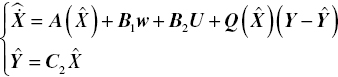
where ![]() is the state vector of the observer; Ŷ is the observer output; and
is the state vector of the observer; Ŷ is the observer output; and ![]() is the output gain. The aim to solve for the observer is to find the output gain
is the output gain. The aim to solve for the observer is to find the output gain ![]() and the detailed solution of the output gain is provided in the reference[15].
and the detailed solution of the output gain is provided in the reference[15].
7.4.4 Simulation Investigation
To demonstrate the effectiveness of the developed integrated control system, a simulation investigation is performed. The vehicle physical parameters are given in Table 7.5 of Section 7.3.12. After tuning, the matrices of the weighting coefficients are selected as:

Figure 7.46 Expected vehicle trajectory input.
The vehicle speed is set as ![]() and the expected input trajectory of the vehicle is illustrated in Figure 7.46. It is observed in the figure that the vehicle travels straight forward first and then around a circle. The stochastic road excitation is applied all the way through, while the lateral wind disturbance is exerted after the vehicle turns and then reaches a steady state condition. In this chapter, it is assumed that the vehicle encounters an abrupt (step) lateral wind disturbance Fw with an amplitude of 1500 N at time
and the expected input trajectory of the vehicle is illustrated in Figure 7.46. It is observed in the figure that the vehicle travels straight forward first and then around a circle. The stochastic road excitation is applied all the way through, while the lateral wind disturbance is exerted after the vehicle turns and then reaches a steady state condition. In this chapter, it is assumed that the vehicle encounters an abrupt (step) lateral wind disturbance Fw with an amplitude of 1500 N at time ![]() , and disappears at time
, and disappears at time ![]() . The proposed integrated control system is compared with the two other systems: only with an EPS (named single EPS), only with an ASS (named single ASS). The following observations are made.
. The proposed integrated control system is compared with the two other systems: only with an EPS (named single EPS), only with an ASS (named single ASS). The following observations are made.
As illustrated in Figure 7.47(a, b; see page 248) and Table 7.6, the peak value of the sideslip angle for the integrated control is reduced by 6.06% and 13.89% respectively, compared with that for the single EPS control and single ASS control, after the steering is applied. In addition, the peak value of the sideslip angle for the integrated control is reduced by 28.99% and 14.04% respectively, after the vehicle encounters the lateral wind. The settling time of the sideslip angle for the integrated control is also decreased for both cases. A similar pattern is observed for the yaw rate. The results indicate that the impact of the abrupt lateral wind disturbance on the vehicle is restrained effectively and hence the vehicle handling stability is improved.
Table 7.6 Responses for handling stability.
| Performance index | Control method | Peak value | Response Time(s) | ||
| Steering | Lateral Wind | Steering angle | Lateral Wind | ||
| Sideslip angle β (rad) | Single EPS control | –0.033 | –0.057 | 2.022 | 4.985 |
| Single ASS control | –0.036 | –0.069 | 2.125 | 5.434 | |
| Integrated system control | –0.031 | –0.049 | 2.018 | 4.751 | |
| Yaw rate r (rad.s–1) | Single EPS control | 0.215 | 0.342 | 1.851 | 4.895 |
| Single ASS control | 0.238 | 0.716 | 1.878 | 5.284 | |
| Integrated system control | 0.212 | 0.289 | 1.845 | 3.826 | |
It is observed clearly in Figure 7.47(c) and Table 7.7 that the peak value of the steering torque for the integrated control is reduced by 8.78% and 16.18% respectively, compared with that for the single ASS control and single EPS control. In addition, the steady state value of the steering torque for the integrated control is reduced by 13.45% and 14.96% respectively, and the settling time is decreased by 8.22% and 10.32% respectively. The results demonstrate that the integrated control system is able to maintain both steering agility and good road feel, and at the same time effectively restrain the impact of the abrupt lateral wind disturbance on the vehicle.
Table 7.7 Steering torque.
| Control Method | Maximum (Nm) | Response Time (s) | Steady State Value (Nm) | |||
| Steering | Lateral Wind | Steering | Lateral Wind | Steering | Lateral Wind | |
| Single EPS control | 45.85 | 22.17 | 1.005 | 3.589 | 14.93 | 21.38 |
| Single ASS control | 50.26 | 27.86 | 1.095 | 3.455 | 17.25 | 23.55 |
| Integrated system control | 42.13 | 21.91 | 0.982 | 3.398 | 14.67 | 21.11 |

Figure 7.47 Comparisons of the responses for the three control systems. (a) Sideslip angle. (b) Yaw rate. (c) Steering torque. (d) PSD of vehicle vertical acceleration. (e) Vehicle vertical acceleration. (f) Suspension deflection. (g) Roll angle. (h) Pitch angle.
Figure 7.47(d–h) and Table 7.8 illustrate that these performance indices on ride comfort, including the vehicle vertical acceleration, roll angle, pitch angle and suspension deflection, are reduced for the integrated control, compared with that for the single ASS control and single EPS control. For brevity, the vehicle vertical acceleration is selected to show the improvement of the integrated control system over the other two control systems. As shown in Figure 7.47(d), the PSD (power spectrum density) value of the vehicle vertical acceleration for the integrated control is decreased significantly compared with the single EPS control in the human body-sensitive frequency region of 1–12 Hz. Moreover, it is observed that the PSD value for the integrated control is decreased greatly in the frequency region of 8–12 Hz compared with the single ASS control, although there is no big difference between the two in the frequency region of 1–4 Hz, which is the resonant frequency region of the sprung mass. Therefore, the results indicate that the vehicle ride comfort is improved significantly by the integrated control system compared with both the single EPS and single ASS control systems.
Table 7.8 Response for ride comfort.
| Performance index | Control method | Average | Root mean square |
| Acceleration zc (m.s–2) | Single EPS Control | 0.0130 | 0.9115 |
| Single ASS Control | 0.0087 | 0.8273 | |
| Integrated System Control | 0.0070 | 0.7757 | |
| Roll angle ø (rad) | Single EPS Control | 0.0923 | 0.0747 |
| Single ASS Control | 0.0586 | 0.0458 | |
| Integrated System Control | 0.0521 | 0.0349 | |
| Pitch angle θ (rad) | Single EPS Control | 0.0069 | 0.0097 |
| Single ASS Control | 0.0065 | 0.0085 | |
| Integrated System Control | 0.0061 | 0.0081 | |
| Suspension deflection fd (m) | Single EPS Control | 0.0222 | 0.0115 |
| Single ASS Control | 0.0189 | 0.0083 | |
| Integrated System Control | 0.0176 | 0.0076 |
7.5 Integrated Control of Active Suspension System (ASS) and Electric Power Steering System (EPS) using the Predictive Control Method
Predictive control (or model predictive control (MPC)) theory is an advanced control method developed from an industrial process control used in the 1980s. The principle behind predictive control is to use the past and current system states to predict the future change of the system output. The system’s optimal control is achieved by minimizing the error between the controlled variables and the targets by applying an iterative, finite time-horizon optimization approach. The predictive control method is applied to the integrated control of the ASS and EPS systems in this chapter[29] since the predictive control has advantages in dealing with both soft and hard constraints, and uncertainties in a complex multivariable control framework.
7.5.1 Designing a Predictive Control System
As developed in the previous chapter, the same 7-DOF vehicle dynamic model is used. To apply the iterative, finite time-horizon optimization approach, the control system model must be represented by a discrete state equation[29]. The system predictive width is set as P, and the control width C must follow the condition ![]() . The optimization objective of the system between the reference trajectory r(k) and the model predictive output y(k) is given in a quadratic form:
. The optimization objective of the system between the reference trajectory r(k) and the model predictive output y(k) is given in a quadratic form:
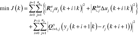
where R and Q correspond to the weighting matrices of the control variables and output variables, respectively, and ![]() ,
, ![]() ,
, ![]() ; nu and ny are the dimensions of the control variables and output variables;
; nu and ny are the dimensions of the control variables and output variables; ![]() are the weighting coefficients of the control variables,
are the weighting coefficients of the control variables, ![]() are the weighting coefficients of the variation rates of the control variables,
are the weighting coefficients of the variation rates of the control variables, ![]() correspond to the weighting coefficients of system outputs; and
correspond to the weighting coefficients of system outputs; and ![]() are the predicted outputs at time k and step
are the predicted outputs at time k and step ![]() .
.
The predictive control is based on the iterative, finite time-horizon optimization of the system model. At every sample time, the constrained optimization problem defined in equation (7.78) is solved online. Only the first term of the control sequence ![]() is implemented to the control variables, then the system’s states are sampled again and the optimization process is repeated starting from the new current states. The prediction horizon keeps being shifted forward, and for this reason MPC is also called receding horizon control. The block diagram of the proposed predictive control system is shown in Figure 7.48[30].
is implemented to the control variables, then the system’s states are sampled again and the optimization process is repeated starting from the new current states. The prediction horizon keeps being shifted forward, and for this reason MPC is also called receding horizon control. The block diagram of the proposed predictive control system is shown in Figure 7.48[30].

Figure 7.48 Block diagram of the predictive control system.
7.5.2 Boundary Conditions
One of the advantages of predictive control is the ability to explicitly handle the boundary conditions of the control variables in a multivariable control framework, and then predict the future output and take the control actions accordingly by applying online the iterative, finite horizon optimization approach. The major boundary conditions are defined as follows by considering the control requirements of the integrated EPS and ASS control system[31]:
- The collision between the suspension and the frame/body should be avoided. The dynamic travel of the suspension should be constrained by its mechanical structure:
(7.79)

 is the suspension deflection at each suspension; and fdmax is the maximum dynamic deflection of the suspension. It is usually selected as 7–9 cm for sedans, 5–8 cm for buses, and 6–9 cm for commercial vehicles.
 - Tyre–road contact must be ensured in order to provide enough lateral and longitudinal forces to the vehicle. Hence, the dynamic load of the tyre does not exceed the static load.
(7.80)

 is the dynamic displacement of each tyre; and kti is the tyre stiffness.
 - When the vehicle lateral acceleration reaches 0.4 g, the roll angle is selected as
 for sedans, and not greater than
  for commercial vehicles.
 - The vehicle lateral acceleration should not exceed 0.6 g, the yaw rate should not exceed 0.6 rad/s, and the pitch rate should not exceed 0.3 rad/s.
- The active suspension force and the steering torque Tm of the EPS is also constrained:
(7.81)
 (7.82)
7.5.3 Simulation Investigation
To demonstrate the effectiveness of the developed integrated control system, a simulation investigation is performed. It is assumed that the vehicle speed uc is 20 m/s; the steering wheel input is a step function with an amplitude of π/2; the predictive width P selected as 10, and the control width C as 4; and the sampling time is 0.005 s. After tuning, the weighting coefficients are selected as: q1 = q2 = 103, q3=100, q4=500, q5= q6=1, q7 = q8 = q9 = q10 = 400, q11 = q12 = q13 = q14 = 103, r11 = r21 = r31 = r41 =10–3, r51=10–2, r12 = r22 = r32 = r42 = r52=1. The integrated control is compared with the non-integrated control (i.e., the EPS and ASS subsystem controllers work independently), and the passive system to demonstrate the performance of the integrated control system.


Figure 7.49 Comparisons of the responses for the three systems. (a) Yaw rate. (b) Pitch angular acceleration. (c) Lateral acceleration. (d) Vertical acceleration. (e) Dynamic deflection of the front suspension (left and right).
It is observed in Figure 7.49(a–e) that the vehicle multiple performance indices for the integrated controlare reduced to various extents compared with the non-integrated control. The results indicate that the integrated control system based on the proposed predictive control is able to improve the overall vehicle performance, including handling stability and ride comfort, by coordinating the interactions between the ASS and EPS.
In addition, a sensitive study is performed to investigate the influence of the predictive width and control width. Figure 7.50 illustrates that control stability and robustness are increased as the predictive width P increases, but the dynamic response is slow. Moreover, as the control width C increases, the dynamic response becomes faster, and the control sensitivity is improved correspondingly, but the system stability is reduced.

Figure 7.50 Influence of the predictive width and control width. (a) Predictive width variation. (b) Control width variation.
7.6 Integrated Control of the Active Suspension System (ASS) and Electric Power Steering System (EPS) using a Self-adaptive Control Method
In practice, numerous uncertainties exist in vehicle dynamics models, including stochastic excitations from the road surface, time-varying physical parameters of the vehicle, disturbances of the lateral wind, and measurement noises of on-vehicle sensors. In recent years, self-adaptive control has been identified as an attractive and effective control method to control systems with uncertainties. Self-adaptive control, which has a long history in the field of control engineering, is an advanced control method where the controller is able to adapt to a controlled system with uncertainties. The SISO self-tuning regulator was first proposed in 1973, and then the self-tuning regulator and controller were extended to MIMO in the 1980s. As a result, a number of multivariable self-tuning control methods were developed by combining the recursive parameter estimation method and minimum variance regulation law, generalized minimum variance regulation law, pole placement control law, feed forward control law, and so on. In this chapter, self-adaptive control is applied to the integrated EPS and ASS control by combining the recursive least square estimation method and the generalized minimum variance control law[32,33]. The block diagram of the self-adaptive integrated control system is illustrated in Figure 7.51.

Figure 7.51 Block diagram of the self-adaptive control system for the integrated EPS and ASS control.
7.6.1 Parameter Estimation of a Multivariable System
The foundation of the self-adaptive control method is parameter estimation. The parameter estimation of the multivariable integrated control system is performed according to the following steps. First, the integrated control system is simplified as a linear multivariable system, and the outputs of the two ASS and EPS subsystems are relatively independent. The outputs of the two subsystems have effects on vehicle performance including vertical acceleration, roll angle, yaw rate, etc. Therefore, if the system noise ξ(t) given in equation (7.83) is an irrelevant measured noise with a mean of zero and variance of σ2, the multivariable integrated control system is considered as a system consisting of m independent SIMO (single input multiple outputs) subsystems[21]. Thereafter, the parameter estimation equation of the multivariable system is decomposed into a set of parameter estimation equations, each of them corresponding to a SIMO subsystem. Finally, the recursive modified least square method is applied to the parameter estimation equations for the multiple SIMO subsystems, and hence the model parameters are obtained.
7.6.2 Design of the Multivariable Generalized Least Square Controller
The ARMAX model of the deterministic linear multivariable system is given as:
where ![]() and
and ![]() are the polynomial matrices of the unit backward shift operator
are the polynomial matrices of the unit backward shift operator ![]() ; u(t) and y(t) are the input and output vectors with dimension of n; da is the steady state error vector with dimension of n; and ξ(t) is the system noise. The generalized output vector is defined as:
; u(t) and y(t) are the input and output vectors with dimension of n; da is the steady state error vector with dimension of n; and ξ(t) is the system noise. The generalized output vector is defined as:
And the generalized ideal output vector is defined as:
where ![]() , and
, and ![]() are the weighted polynomial matrices of
are the weighted polynomial matrices of ![]() ; T(z) is the lower triangle matrix of z; and p(t) is the n-dimensional reference input vector with known boundary.
; T(z) is the lower triangle matrix of z; and p(t) is the n-dimensional reference input vector with known boundary.
If the optimal prediction of the generalized output vector ![]() equals the generalized ideal output
equals the generalized ideal output ![]() , the generalized minimum variance control law is obtained as:
, the generalized minimum variance control law is obtained as:
And the system performance factor J reaches the minimum:
where Ft denotes the non-descending σ-algebraic group; and ![]() is the polynomial matrix of
is the polynomial matrix of ![]() .
.
7.6.3 Design of the Multivariable Self-adaptive Integrated Controller
The multivariable self-adaptive integrated controller is designed according to the following steps[34]:
- Measure the real output y(t) and external input p(t) at time t;
- Compute
 ;
; - Construct the vectors
 and
and  ;
; - Calculate the estimate parameter matrix
 ;
; - Compute the new control input u(t);
- Go back to step (1), add one to the time counter and repeat the steps above.
7.6.4 Simulation Investigation
To demonstrate the effectiveness of the developed integrated control system, a simulation investigation is performed. The vehicle physical parameters are the same as those defined in Section 7.3.12. The maneuver of step steering input is applied and the vehicle speed uc is assumed to be 10 m/s and 20 m/s, respectively. The generalized ideal output of the system can be obtained as follows: The roll angle φ is expected to be as small as possible, and the yaw rate r is expected to reach an expected steady state value rd. The self-adaptive integrated control is compared with the single EPS control and the single ASS control to demonstrate the performance of the integrated control system.
It is observed in Tables 7.9 and 7.10 that the self-adaptive integrated control system performs the best among the three control systems on the performance indices of the peak value and settling time of both the vehicle yaw rate and roll angle. The results indicate that both the handling stability and ride comfort are improved through applying the self-adaptive control method to the integrated EPS and ASS control. In addition, the results show that the application of the self-adaptive control method is able to reduce effectively the effects of both the model uncertainties and stochastic disturbances on the system. Moreover, comparisons between the single EPS and ASS demonstrate that the single ASS is able to maintain the vehicle attitude more effectively than the single EPS control under the maneuver of step steering input.
Table 7.9 Comparison of the peak value of responses.
| Performance index | EPS control | ASS control | Integrated control | EPS control | ASS control | Integrated control |
| Yaw rate/r ( |
0.17 | 0.15 | 0.12 | 0.22 | 0.20 | 0.18 |
| Roll angle/φ (rad) | 0.41 | 0.032 | 0.029 | 0.11 | 0.068 | 0.016 |
Table 7.10 Comparison of settling time responses.
| Settling time of performance index | EPS control | ASS control | Integrated control | EPS control | ASS control | Integrated control |
| Yaw rate (s) | 0.43 | 0.37 | 0.20 | 0.9 | 0.58 | 0.30 |
| Roll angle (s) | 1.7 | 1.2 | 1.0 | 1.6 | 1.2 | 1.0 |
7.7 Integrated Control of an Active Suspension System (ASS) and Electric Power Steering System (EPS) using a Centralized Control Method
This section studies the integrated control of electric power steering system (EPS) and active suspension system (ASS) to achieve the goal of function integration of the control systems[35]. The nonlinear centralized control theory is applied to design a centralized controller in order to solve the system couplings between the ASS and EPS, and eliminate the disturbances from the road excitations. Moreover, a centralized PD controller is designed based on the centralized vehicle dynamic system in order to improve the dynamic responses of steering conditions.
7.7.1 Centralized Controller Design
7.7.1.1 Centralization of System Inertial Term
This study uses the same models as those developed in Section 7.4, including the nonlinear vehicle dynamic model, EPS system model, and ASS model.
The nonlinear dynamic model is transformed into the affine nonlinear form described in reference[36] through order reduction of the differential equation and centralized of the inertial terms. The state equation of the system is given as:
where ![]() is the coefficient matrix;
is the coefficient matrix; ![]() is the input matrix; Δf(x, t) is the affine nonlinear term of the state variables; and P is the disturbance coefficient matrix. The output equation is given as
is the input matrix; Δf(x, t) is the affine nonlinear term of the state variables; and P is the disturbance coefficient matrix. The output equation is given as
where ![]() is the output coefficient matrix. The control variables include the control forces of the active suspension
is the output coefficient matrix. The control variables include the control forces of the active suspension ![]() , and the assist torque provided by the motor of the EPS. Therefore, the control input vector is defined as:
, and the assist torque provided by the motor of the EPS. Therefore, the control input vector is defined as:
The multiple vehicle performance indices are considered to evaluate both the vehicle handling stability and ride comfort. These performance indices can be measured by the following physical terms: the vertical acceleration of the sprung mass ![]() ; the roll angle Φ; the suspension dynamic deflection fd; the yaw rate r; and the sideslip angle β. Therefore, the output vector is defined as:
; the roll angle Φ; the suspension dynamic deflection fd; the yaw rate r; and the sideslip angle β. Therefore, the output vector is defined as:
For the above system with the same number of input variables and output variables, the static state feedback decouple method is used. For brevity, the detailed derivations of the matrices ![]() ,
, ![]() ,
, ![]() ,
, ![]() ,
, ![]() , x and the affine nonlinear term Δf(x, t) are not presented here.
, x and the affine nonlinear term Δf(x, t) are not presented here.
7.7.1.2 Centralized System
Let ![]() . It can be proven that the other
. It can be proven that the other ![]() transformations can be found to construct the following mapping:
transformations can be found to construct the following mapping:
where ![]() is the relative degree of the system; Lfλ(x) is a scalar function; f(x) and λ(x) are the functions of x. Please refer to Section 7.3 or reference[36] for the definitions of these functions. Thus, the transformation of the local coordinates at
is the relative degree of the system; Lfλ(x) is a scalar function; f(x) and λ(x) are the functions of x. Please refer to Section 7.3 or reference[36] for the definitions of these functions. Thus, the transformation of the local coordinates at ![]() is constructed as:
is constructed as:
The defined system output is the last row of the first five sub-matrix. It is given as:

Combining this with the feedback control law u, the subsystem is given as:

Therefore, the matrix constructed by ![]() is expressed as:
is expressed as:

i.e.

and the system output ![]() . Therefore, the centralized of the control channels is fulfilled since every control signal vi only controls the system output
. Therefore, the centralized of the control channels is fulfilled since every control signal vi only controls the system output ![]() through a series of integrators with an order of ri. However, it should be noted that the system output yi is not only affected by vi, but also by the road excitations. In fact, the control signal vi does not have any physical meaning, in contrast to the feedback control law u as defined in equation (7.89).
through a series of integrators with an order of ri. However, it should be noted that the system output yi is not only affected by vi, but also by the road excitations. In fact, the control signal vi does not have any physical meaning, in contrast to the feedback control law u as defined in equation (7.89).
Based on the centralized control theory, the system should be separated into the subsystems with independent control channels to derive the feedback control law. Therefore, the relative degree of the affine nonlinear system is needed. Then, the system can be transformed into a serial structure that consists of a number of subsystems with the degree of ![]() and the integrators. Refer to Section 7.3 or reference[35] for the detailed derivation of the relative degree, the design of the input–output centralized controller, and the design of the disturbance centralized controller.
and the integrators. Refer to Section 7.3 or reference[35] for the detailed derivation of the relative degree, the design of the input–output centralized controller, and the design of the disturbance centralized controller.
7.7.1.3 Centralized PD Controller Design
The control channels become independent and the disturbance from the road excitations are subdued after the system is centralized. However, the response quality of system is not improved significantly since the control signal vi is not tuned. The response quality of the system includes the settling time, overshoot, and response error. To further improve the response quality of the system, a PD control law is introduced, and the control signal vi becomes:
where e and de are the error of the output signal and the difference of the error, respectively; Kp and Kd are the vector of the proportional coefficient and differential coefficient, respectively.
Finally, the block diagram of the centralized PD control system is shown in Figure 7.52. In the figure, the reference input for the system is defined as:
The above steady-state parameters are calculated by using equation (7.90) when the step steering is selected as the steering wheel input.
Figure 7.52 Block diagram of the centralized PD control system.
7.7.2 Simulation Investigation
A simulation investigation is performed to demonstrate the performance of the proposed centralized PD control system. We assume that the vehicle travels at a constant speed ![]() , and the step steering input
, and the step steering input ![]() . A filtered white noise signal[37] is selected as the road excitation to the vehicle. The vector of proportional coefficient and differential coefficient is selected as
. A filtered white noise signal[37] is selected as the road excitation to the vehicle. The vector of proportional coefficient and differential coefficient is selected as ![]() and
and ![]() . For comparison, two simulation studies are performed. The first is to compare to the system using the PD control and centralized control, and the other is to compare to the non-integrated systems, i.e., the ASS-only system and EPS-only system. The following discussions are made from the simulation results shown in Figures 7.53–7.59 and Table 7.11:
. For comparison, two simulation studies are performed. The first is to compare to the system using the PD control and centralized control, and the other is to compare to the non-integrated systems, i.e., the ASS-only system and EPS-only system. The following discussions are made from the simulation results shown in Figures 7.53–7.59 and Table 7.11:
- It is clearly observed from Figure 7.53 and Figure 7.54 that both the vertical acceleration of the sprung mass and the dynamic deflection of the front-right suspension for the proposed centralized PD control system are greatly reduced compared to that for both the PD control system and the centralized control system. It can be obtained through a quantitative analysis on the simulation results that the percentage decrease of the vertical acceleration of the spring mass is 65.1 and 27.6, and of the dynamic deflection is 44.2 and 30.8. It should be noted that the dynamic deflection of the front-right suspension is taken as an example since similar patterns can be observed for the other three suspensions. The results indicate that vehicle ride comfort is improved significantly by the proposed centralized PD control system in comparison with the other two control systems since the proposed control system integrates the advantages of the PD control and centralized control to eliminate effectively the disturbance from the road excitation.
- The performance indices on lateral stability are also shown in Figures 7.55–7.57 and Table 7.11. Compared to both the PD control system and the centralized control system, the sideslip angle of the sprung mass, the sideslip angle of the vehicle, and the yaw rate are reduced by the proposed centralized PD control system. The results indicate that lateral stability is improved by the proposed centralized PD control system.
- It is observed clearly from Figure 7.58 and Figure 7.59 that both the vertical acceleration of the sprung mass and the dynamic deflection of the suspension for the proposed centralized PD control system are reduced significantly compared to that for both the ASS-only PD control system and the EPS-only PD control system. The results indicate that vehicle ride comfort is improved by the proposed centralized PD control system since the proposed control system is able to coordinate the EPS and ASS to achieve integration between the two systems.
Table 7.11 Simulation results.
| Control method | Peak value of response | Overshoot % | Response time (s) | |
| Sideslip angle of vehicle | PD control | 0.1446 | 27.36 | 0.783 |
| Centralized control | 0.1484 | 30.76 | 0.834 | |
| Centralized PD control | 0.1421 | 25.18 | 0.745 | |
| Sideslip angle of sprung mass | PD control | 0.0800 | 12.68 | 0.436 |
| Centralized control | 0.0082 | 15.49 | 0.482 | |
| Centralized PD control | 0.0078 | 9.86 | 0.412 | |
| Yaw rate | PD control | –0.0286 | 28.63 | 0.423 |
| Centralized control | –0.0338 | 52.42 | 0.482 | |
| Centralized PD control | –0.0282 | 26.87 | 0.423 |

Figure 7.53 Vertical acceleration of the sprung mass (Front-right suspension).

Figure 7.54 Dynamic deflection.

Figure 7.55 Sideslip angle of the sprung mass.

Figure 7.57 Yaw rate.

Figure 7.58 Vertical acceleration of the sprung mass.

Figure 7.59 Dynamic deflection.
7.8 Integrated Control of the Electric Power Steering System (EPS) and Vehicle Stability Control (VSC) System
This section studies the integrated control of the electric power steering system (EPS) and the vehicle stability control (VSC) system to achieve the goal of integrating the two control systems. The aim of the study is to design a new control strategy to compensate the return torque of the EPS system by considering the interactions of the VSC system under critical driving conditions.
7.8.1 Interactions Between EPS and VSC
The interactions between the EPS and VSC arise from the lateral forces of the tyres provided by the road surface. When we design the EPS separately, i.e., without taking into account the interactions of the VSC, the assist torque is determined mainly through calculating the return torque of the two front tyres. However, when the vehicle is under critical driving conditions, the lateral forces between the tyres and the road reach saturation, and the VSC intervenes to change the longitudinal forces of the tyres and thus change the lateral forces of the tyres. This results in the change of the return torque from the tyres. Therefore, it is necessary to design a new control strategy to compensate for the return torque by considering the intervention of the VSC.
7.8.2 Control System Design
The block diagram of the integrated control system is shown in Figure 7.60. The work principle of the proposed integrated control system is described as follows: in the VSC control unit, the reference inputs for the vehicle dynamic system, including the expected longitudinal speed of the vehicle ud, expected lateral speed vd, and expected yaw rate rd, are calculated from the vehicle 2-DOF reference model. Then, a nonlinear sliding mode controller is used to calculate the expected control force Fud in order to track the desired vehicle motions. The expected control force ![]() is defined as a vector of the expected forces for vehicle stability control, where Fxd, Fyd, Mzd is the expected longitudinal force, expected lateral force, and expected yaw moment, respectively. Thereafter, the expected control force Fud is distributed optimally to the four wheels. The actual return torque is then generated based on the lateral forces of the two front wheels. In the EPS control unit, the compensated assist torque is obtained by comparing the desired return torque with the actual return torque in the return torque controller. The assist torque Ta is finally calculated by the assist torque controller. Therefore, the lateral stability of the vehicle is improved by compensating the return torque and considering the intervention of the VSC under critical driving conditions.
is defined as a vector of the expected forces for vehicle stability control, where Fxd, Fyd, Mzd is the expected longitudinal force, expected lateral force, and expected yaw moment, respectively. Thereafter, the expected control force Fud is distributed optimally to the four wheels. The actual return torque is then generated based on the lateral forces of the two front wheels. In the EPS control unit, the compensated assist torque is obtained by comparing the desired return torque with the actual return torque in the return torque controller. The assist torque Ta is finally calculated by the assist torque controller. Therefore, the lateral stability of the vehicle is improved by compensating the return torque and considering the intervention of the VSC under critical driving conditions.

Figure 7.60 Block diagram of the integrated control system.
7.8.3 Dynamic Distribution of Tyre Forces
As mentioned above, the expected control force Fud must be distributed optimally to the four wheels. The distribution of the tyre forces is a multivariable constrained optimization problem, subjected to the distribution accuracy among the four wheels and the control energy. A dynamic distribution method is applied to the distribution of the tyre forces according to the error between the actual value and the expected value of the yaw moment[38].
The compositions of the longitudinal and lateral forces and the yaw moment should have certain limits since the tyre–road friction forces cannot exceed the adhesion limits. Moreover, the feasible regions for the composition of forces and yaw moment are not rectangles since the longitudinal and lateral forces are coupled. When the composition of the longitudinal forces is determined, the yaw moment varies with the different distributions of the longitudinal forces of the four wheels. If all the possible distributions of the longitudinal forces are defined as a set, the yaw moment can be defined as a function of the set. The values of such a function can be constructed into a set with certain limits. When the composition of the longitudinal forces is determined, the upper limit of the functional set can be obtained. Therefore, a curve can be determined to describe the relation that the upper limits of the functional set vary with the different compositions of the longitudinal forces. The curve is defined as the feasible region of the composition of the longitudinal forces and the yaw moment. When the vehicle drives at high speeds, the steering angles of the front wheels are small and hence can be ignored. Thus, the compositions of forces and yaw moment are obtained as follows:
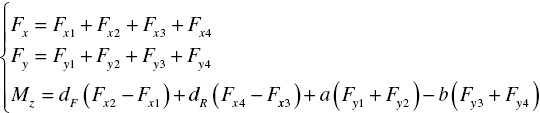
where the subscripts 1 through 4 represent the left-front, right-front, left-rear, and left-front wheels, respectively; dF, dR represent half of the front and rear wheel track, respectively; a, b represent the distance of the front axle and rear axle between the C.G., respectively; Fx, Fy, and Mz represent the compositions of the longitudinal and lateral forces, and the yaw moment, respectively.
The distributions of the compositions of forces and the yaw moment are given as follows. First, the composition of the longitudinal forces is distributed. The error of the yaw moment is defined as:
The additional yaw moment resulting from the longitudinal forces is obtained from equation (7.95),
Let the additional yaw moment be:
Therefore, the error of the yaw moment eM can be compensated by the additional yaw moment by selecting a suitable coefficient k1. A constrained quadratic programming problem is defined as follows:

where ![]() are the maximum tyre road friction forces;
are the maximum tyre road friction forces; ![]() , where Fzi is the vertical load of the tyre; and k2, k3, k4, k5 are the function distribution coefficients for the longitudinal forces. However, the above equation cannot compensate accurately for the error of the yaw moment since the longitudinal and lateral forces of the front wheels are coupled. Hence, it is necessary to adjust the lateral forces of the front wheels to further improve the track error of the yaw moment.
, where Fzi is the vertical load of the tyre; and k2, k3, k4, k5 are the function distribution coefficients for the longitudinal forces. However, the above equation cannot compensate accurately for the error of the yaw moment since the longitudinal and lateral forces of the front wheels are coupled. Hence, it is necessary to adjust the lateral forces of the front wheels to further improve the track error of the yaw moment.
It can be observed that the additional yaw moment resulting from the lateral forces of the two front wheels is actually related to the composition of the two forces. Therefore, let the composition of the two forces be ![]() , and FyF at the k-th sampling time is given as:
, and FyF at the k-th sampling time is given as:
where k6 is a constant. Finally, the lateral force of each front tyre is determined according to its proportion of the vertical load:

7.8.4 Design of a Self-aligning Torque Controller
In order to design a self-aligning torque controller, an analysis of the relationship between the vehicle self-aligning torque and sideslip angle is performed. Figure 7.61 shows the relationship for the 7-DOF vehicle dynamic model by assuming that the vehicle speed is a constant of 72 km/h and the road adhesion coefficient is 0.3. It is observed in Figure 7.61 that the self-aligning torque is approximately proportional to the sideslip angle when the sideslip angle is small, and it reaches the maximum when the sideslip angle is around 4°–6°. As the sideslip angle keeps increasing, the self-aligning torque is decreased instead. Under this circumstance, the hand torque required by the vehicle driver is increased, and also the road feel is lost. Therefore, the compensation of the self-aligning torque is required through adjusting the EPS based on the vehicle states obtained from VSC system.

Figure 7.61 Relationship between self-aligning torque and sideslip angle.
The compensation value of the self-aligning torque for the EPS varies with the lateral force. The reason is that the self-aligning torque varies with respect to the sideslip angle. Moreover, the lateral forces also change when the VSC intervenes. Therefore, the PID fuzzy control is used to regulate the compensation value of the self-aligning torque in real time to track the expected value in order to design an appropriate self-aligning torque controller. As shown in Figure 7.62, the fuzzy controller has two input variables: the tracking error of the self-aligning torque τ, and the difference of the error ![]() . The three tuning parameters KP , KI , and KD are selected as the outputs of the fuzzy controller, and they are the inputs of the PID controller. The application of the PID controller is to guarantee that the actual self-aligning torque tracks the expected one in real time.
. The three tuning parameters KP , KI , and KD are selected as the outputs of the fuzzy controller, and they are the inputs of the PID controller. The application of the PID controller is to guarantee that the actual self-aligning torque tracks the expected one in real time.

Figure 7.62 Control system chart of the self-aligning torque.
The actual self-aligning torque is calculated as:
where M1, M2 are the self-aligning torques of the vehicle front-left and front-right wheels, respectively; and e1, e2 are the pneumatic trails of the two front tyres, respectively. The expected self-aligning torque is derived as:

where Mc is the expected self-aligning torque; ![]() is the slope rate of the self-aligning torque with respect to the sideslip angle when the linear relationship between them holds; and αi is the actual sideslip angle of the two front wheels. The rule bases of the fuzzy controller are developed for the three output variables KP, KI, and KD with respect to the input variable τ and its difference
is the slope rate of the self-aligning torque with respect to the sideslip angle when the linear relationship between them holds; and αi is the actual sideslip angle of the two front wheels. The rule bases of the fuzzy controller are developed for the three output variables KP, KI, and KD with respect to the input variable τ and its difference ![]() as follows:
as follows:
- For a relatively large τ, a relatively larger KP is selected to eliminate deviations and increase the response speed as soon as possible. In the meantime, KI is set as zero to avoid large overshoots.
- For a relatively small τ, KP must be reduced and KI should be a relatively small value to continue to reduce the deviations and also to prevent large overshoots and oscillations.
- For an extremely small τ, KP should keep decreasing and KI should remain constant or increase a little to eliminate steady errors, and overcome the overshoots and stabilize the system as soon as possible.
- When the signs of τ and
 are the same, it means that the controlled variables vary away from the target values. Therefore, when the controlled variables approach the target values, the proportional parameter with the opposite sign counteracts the effects of the integral parameter to avoid the overshoots and the subsequent oscillations resulted from the integral parameter. While the control variables are far from the target values and vary towards them, the control process slows down due to the opposite signs of τ and
  . Therefore, when τ is relatively large and the signs of
  and τ are opposite, KI is selected to be zero or negative to accelerate the control process.
 - The value of
 shows the change rate of the tracking error. As
  becomes larger, KP should become smaller and KI larger, and vice versa. At the same time, the value of τ should also be taken into consideration.
 - The differential parameter KD is used to improve the system dynamic characteristics and prevent the variation of τ. The differential parameter KD is beneficial to reduce overshoots, eliminate oscillations, and shorten the settling time. Therefore, KD should be increased to reduce the system steady state error and hence improve the control accuracy. When τ is relatively large, KD is selected to be zero, and the controller becomes a PI controller; when τ is relatively small, KD is selected to be medium, resulting in a PID control.
To design the fuzzy controller, τ and ![]() are selected as the input language variables, the fuzzy subset of each variable is set as {Negative Big, Negative Medium, Negative Small, Zero, Positive Small, Positive Medium, Positive Large}, which is denoted as{NB,NM,NS,ZO,PS,PM,PB}. The discourse domains of both τ and
are selected as the input language variables, the fuzzy subset of each variable is set as {Negative Big, Negative Medium, Negative Small, Zero, Positive Small, Positive Medium, Positive Large}, which is denoted as{NB,NM,NS,ZO,PS,PM,PB}. The discourse domains of both τ and ![]() are defined as {–3,–2,–1,0,1,2,3}. The triangular full overlap function is adopted as the membership function, and the Sum-Product rule is used for fuzzy inference. The membership function of each rule is denoted as
are defined as {–3,–2,–1,0,1,2,3}. The triangular full overlap function is adopted as the membership function, and the Sum-Product rule is used for fuzzy inference. The membership function of each rule is denoted as ![]() . Therefore, the three output variables are obtained by the weighted mean method:
. Therefore, the three output variables are obtained by the weighted mean method:
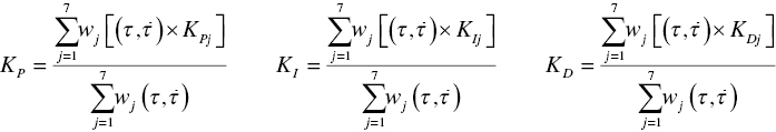
where KPj, KIj, and KDj are the weighed parameters of KP, KI, and KD under different conditions. Therefore, the output of the fuzzy PID controller, i.e., the compensation of the self-aligning torque, is obtained as:
7.8.5 Simulation Investigation
To validate the effectiveness of the compensation strategy of the self-aligning torque, a simulation is performed by comparing the integrated control of the VSC and EPS with the non-VSC control, and VSC control. The vehicle initial speed is set as 72 km/h, and a low road adhesion coefficient of 0.3 is selected. Two driving conditions are performed, including the step steering input and single lane change.

Figure 7.63 Comparison of responses for the maneuver of a single lane change. (a) Single lane change steering input to the front wheel. (b) Yaw rate. (c) Sideslip angle.

Figure 7.64 Comparison of responses for the maneuver of a step steering input. (a) Step steering input to the front wheel. (b) Yaw rate. (c) Sideslip angle.
It is observed in Figures 7.63 and 7.64 that the integrated control system of VSC and EPS performed the best amongst the three systems considered on both the yaw rate and the sideslip angle. In addition, the application of the compensation strategy of the self-aligning torque is able to track the reference value faster and, hence, the settling time is shorter compared with the VSC control. Therefore, vehicle handling stability is improved by the integrated control of VSC and EPS.
7.9 Centralized Control of Integrated Chassis Control Systems using the Artificial Neural Networks (ANN) Inverse System Method
In recent years, intelligent control methods have been applied widely to the centralized control of multivariable systems to deal with nondeterministic and complex control problems. This study takes advantage of both the neural network and the centralized linearization of the inverse system. As a result, the neural network inverse system method is applied to the integrated control of vehicle Active Front Steering (AFS), Direct Yaw moment Control (DYC), and Active Suspension System (ASS)[26,39].
7.9.1 Vehicle Dynamic Model
As described above in Section 7.3, the nonlinear centralized method was applied to the integrated control of VSC and ASS. The overall vehicle performance, including handling stability and comfort, was improved by regulating the vertical load distribution and adjusting the brake forces. In this section, the AFS system is designed to serve as a steering correction system by applying an additional steer angle to the driver’s steering input in the linear handling region. In this way, the AFS system is able to improve steerability by assisting the driver in handling the vehicle and preventing extreme handling situations. In this study, the integrated control VSC and ASS system is integrated further with the AFS system, and the neural network inverse system method is used to design the integrated centralized control of the AFS, DYC and ASS. As shown in Figure 7.65, the 7-DOF vehicle dynamic model is used, and the lateral, yaw, and roll motions are considered. In Figure 7.65, uc, β, r, and φ are the vehicle longitudinal speed, sideslip angle, yaw rate, and roll angle, respectively; m, ms, mf, and mr are the vehicle mass, sprung mass, unsprung mass of the front axle, unsprung mass of the rear axle, respectively; a and b are the distances between the center of gravity of the vehicle to the front and rear axles, respectively; Iz, Ix, Ixz are the yaw moment of inertia, roll moment of inertia, and product of inertia of the sprung mass about the roll and yaw axes, respectively ; ![]() and
and ![]() are the lateral stiffnesses of the front and rear tyres, respectively; δF, δc, Tz, and Tφ are the steering angle of the front wheel provided by the driver, additional steering angle to the front wheel provided by the AFS, corrective yaw moment, and suspension roll moment; Kφ and Dφ are the roll stiffness coefficient and damping coefficient of the suspension.
are the lateral stiffnesses of the front and rear tyres, respectively; δF, δc, Tz, and Tφ are the steering angle of the front wheel provided by the driver, additional steering angle to the front wheel provided by the AFS, corrective yaw moment, and suspension roll moment; Kφ and Dφ are the roll stiffness coefficient and damping coefficient of the suspension.

Figure 7.65 Vehicle dynamic model.
The state variable is defined as ![]() , and the control input variable
, and the control input variable ![]() , the system output variable
, the system output variable ![]() , then the state equation of the integrated system is derived as:
, then the state equation of the integrated system is derived as:

where,


It is obvious that equation (7.106) is a typical multivariable system with three inputs and three outputs. Due to the interactions among the tyre’s longitudinal, lateral, and vertical forces, as well as the conflicts among the vehicle translational and rotational motions, the integrated control system of AFS, DYC, and ASS systems is highly coupled. Therefore, it is required to decouple the vehicle multivariable system into three independent SISO control systems in order to design the controller of the integrated system.
7.9.2 Design of the Centralized Control System
7.9.2.1 Analysis of System Invertibility
As described in Section 7.3.6, the Interactor algorithm is used to calculate the relative degree of the integrated control system given in equation (7.106). The detailed calculation of the relative degree is demonstrated as follows.

Let ![]() , the rank of the corresponding Jacobian matrix with respect to input u is:
, the rank of the corresponding Jacobian matrix with respect to input u is:


Let ![]() , the rank of the corresponding Jacobian matrix with respect to u is:
, the rank of the corresponding Jacobian matrix with respect to u is:


Let ![]() , the rank of the corresponding Jacobian matrix with respect to u is:
, the rank of the corresponding Jacobian matrix with respect to u is:
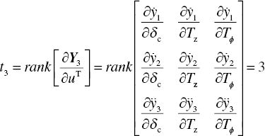
Therefore the relative degree of the system is ![]() , and
, and  (n is the system order). According to the implicit function theorem, it is known that the inverse system of the original integrated control system exists, and the output of the inverse system u (i.e., the input of the original system) is given as:
where ![]() , ϕ(·) is the nonlinear relationship between the input and output of the inverse system. Let
, ϕ(·) is the nonlinear relationship between the input and output of the inverse system. Let ![]() ,
, ![]() ,
, ![]() ,
, ![]() ,
, ![]() ,
, ![]() ,
, ![]() be the inputs to the inverse system, the standard form of the inverse system is given as:
be the inputs to the inverse system, the standard form of the inverse system is given as:

As shown in equation (7.114), a pseudolinear system is constructed by connecting the inverse system ahead of the original one in series, which is equivalent to two first-order integral linear subsystems and one second-order integral linear subsystem. The structure of the pseudo-linear system is illustrated in Figure 7.66.

Figure 7.66 Structure of the pseudo-linear system.
7.9.2.2 Design of a Neural Network Inverse System
The analytical expression of the inverse system given in equation (7.114) is based on the accurate mathematical model. Therefore, the centralized characteristics of the pseudolinear system are realized only if the original system parameters are known, accurate, and time-invariant. To improve the self-adaptability to the parameter variations and the robustness with respect to external disturbances, the static neural network and the integrator is applied to construct the inverse system[25].
It is known from equation (7.114) that the input layer includes β, r, φ, ![]() ,
, ![]() ,
, ![]() , and
, and ![]() ; and the output layer includes δc, Tz, and Tφ. Therefore, the number of neurons on the input layer is set to be seven, and three for the output layer. The number of neurons on the implicit layer is determined to be 15 by the trial-and-error method. The nonlinear mapping of the inverse system is approached by using the static neural network. Four integrators are used to represent the dynamic characteristics of the inverse system. The structure of the developed neural network inverse system is 7-15-3, which is shown in Figure 7.67. In the structure, the function tansig is used as the transfer function for the input layer and the implicit layer of the BP network, and the function purelin for the output layer.
; and the output layer includes δc, Tz, and Tφ. Therefore, the number of neurons on the input layer is set to be seven, and three for the output layer. The number of neurons on the implicit layer is determined to be 15 by the trial-and-error method. The nonlinear mapping of the inverse system is approached by using the static neural network. Four integrators are used to represent the dynamic characteristics of the inverse system. The structure of the developed neural network inverse system is 7-15-3, which is shown in Figure 7.67. In the structure, the function tansig is used as the transfer function for the input layer and the implicit layer of the BP network, and the function purelin for the output layer.

Figure 7.67 Structure of the BP neural network inverse system.

Figure 7.68 Stimulating input signals of neural network inverse system.
It is assumed that the vehicle travels at a speed of 100 km/h, and the driver’s steering input to the front wheels is a sinusoidal curve with a varying amplitude. As shown in Figure 7.68, the stimulating input signals used to train the neural network include the additional angle to the front wheel δc, corrective yaw moment Tz, and roll moment of the suspension Tφ. The dynamic responses of the yaw rate r, sideslip angle β, and roll angle φ are sampled with a period of 5 ms. Then ![]() ,
, ![]() ,
, ![]() and
and ![]() are calculated according to the five-point numerical differential method. Two hundred sets of training data sets [β,
are calculated according to the five-point numerical differential method. Two hundred sets of training data sets [β, ![]() , r,
, r, ![]() , φ,
, φ, ![]() ,
, ![]() ] and [δc, Tz, Tφ] are obtained by combining the above-obtained data. The premnmx function in the neural network toolbox in MATLAB is used to normalize the network input and output data. In the network simulation test, the new data are preprocessed by the function tramnmx in the same way, and finally normalized by the function postmnmx. The BP neural network is established by the function newff, and the function trainlm of the Levenberg-Marquardt algorithm is selected as the training function. The established BP network has been trained by the selected training function for 500 times with a learning efficiency of 0.05, and a network target error of 10–3. The required training accuracy is achieved after 72 sessions training in the simulation.
] and [δc, Tz, Tφ] are obtained by combining the above-obtained data. The premnmx function in the neural network toolbox in MATLAB is used to normalize the network input and output data. In the network simulation test, the new data are preprocessed by the function tramnmx in the same way, and finally normalized by the function postmnmx. The BP neural network is established by the function newff, and the function trainlm of the Levenberg-Marquardt algorithm is selected as the training function. The established BP network has been trained by the selected training function for 500 times with a learning efficiency of 0.05, and a network target error of 10–3. The required training accuracy is achieved after 72 sessions training in the simulation.
7.9.2.3 Design of the PD Controller
By performing the centralized process, the original integrated system is transformed into the three independent SISO systems, including the first-order AFS subsystem, the first-order DYC subsystem, and the second-order ASS subsystem. In order to improve the response quality of the integrated system, a compound controller shown in Figure 7.69 is designed by combining the PD controller and the neural network reverse system.

Figure 7.69 Block diagram of the centralized integrated control system.
As the input and output of the centralized pseudolinear system has a one-to-one linear relationship, a number of control methods for single variable linear systems can be applied to the design of the controller, including PID control, pole placement, and quadratic optimal. Here, the PD closed loop controller is designed as follows:
where e and de are the tracking error of the system output signals, and its difference, respectively; Kp and Kd are the proportional and differential coefficient, respectively. The vehicle reference model included in Figure 7.69, generates the expected dynamic response according to the driver’s input, and the expected sideslip angle and yaw rate are obtained as:

where μ is the road adhesion coefficient, and K is the understeer coefficient.
7.9.3 Simulation Investigation
To demonstrate the effectiveness of the developed integrated control system, a simulation investigation is performed by comparing the developed integrated control system with the integrated control system with PD control, and the system with the decentralized control (i.e., the three stand-alone controllers of AFS, ASS and DYC). The vehicle initial speed is set as uc = 80 km/h, the road adhesion coefficient of ![]() is selected. Two driving conditions are performed, including single lane change and step steering input. The vehicle physical parameters in Table 7.5 are used. After tuning, the PD coefficients of the closed loop controller are set as
is selected. Two driving conditions are performed, including single lane change and step steering input. The vehicle physical parameters in Table 7.5 are used. After tuning, the PD coefficients of the closed loop controller are set as ![]() and
and ![]() . The roll stiffness coefficient of the suspension is
. The roll stiffness coefficient of the suspension is ![]() , and the suspension roll damping coefficient is
, and the suspension roll damping coefficient is ![]() .
.
- (1) Single lane change maneuverThe simulation is performed according to the GB/T6323.1-94 controllability and stability test procedure for automobiles – pylon course slalom test. For the maneuver of a single lane change, the amplitude of the front wheel steering angle is set as 0.08 rad and the frequency as 0.5 Hz. It is illustrated clearly in Figure 7.70 and Table 7.12 that the peak value of the yaw rate for the developed integrated control is reduced greatly by 12% and 29% respectively, compared with the integrated control system with PD control, and the system with the decentralized control. A similar pattern can be observed for the sideslip angle and roll angle. The results indicate that the application of the centralized PD control is able to track effectively the expected vehicle states and hence improve its handling stability.
- (2) Step steering input manoeuvreThe simulation is conducted according to the GB/T6323.2-94 controllability and stability test procedure for automobiles – steering transient response test (steering wheel angle step input). The step steering input to the wheel is set at 1.57 rad. It is illustrated clearly in Figure 7.71 and Table 7.13 that the peak value of the yaw rate for the developed integrated control is reduced significantly by 19.1% and 26.4% respectively, compared with the integrated control system with PD control, and the system with the decentralized control. A similar pattern can be observed for the sideslip angle and roll angle. The results indicate that the application of the centralized PD control is able to track effectively the expected vehicle states and hence improve the vehicle handling stability. In addition, the amplitudes of these performance indices for the combined control system are relatively larger since the conflicts among the three subsystems are unable to coordinate. Finally, these three performance indices for the integrated control system with PD control are deviated from the expected states since the PD controller fails to deal with the coupling effects of the control loop and, hence, it is inevitable that they negatively influence each other.
Table 7.12 Comparison of the peak value of the single line change simulation results.
| Control Method | Yaw rate r/rad. s– 1 | Sideslip angle β/rad | Roll angle φ/rad |
| Expectation | 0.2 | 0.01 | 0 |
| Centralized PD control | 0.22 | 0.041 | 0.075 |
| PD control | 0.25 | 0.062 | 0.096 |
| Decentralized control | 0.31 | 0.081 | 0.147 |
Table 7.13 Comparison of step steering simulation result peak values.
| Control method | Yaw rate r (rad/s) | Sideslip angle β (rad) | Roll angle φ (rad) |
| Reference | 0.2 | 0.017 | 0 |
| Centralized PD Control | 0.195 | 0.055 | 0.096 |
| PD Control | 0.241 | 0.056 | 0.142 |
| Decentralized Control | 0.265 | 0.066 | 0.164 |

Figure 7.70 Comparison of responses for the single lane change maneuver. (a) Yaw rate. (b) Sideslip angle. (c) Roll angle.

Figure 7.71 Comparison of responses for the maneuver of step steering input. (a) Yaw rate. (b) Sideslip angle. (c) Roll angle.
References
- [1] Fruechte R D, Karmel A M, Rillings J H, Schilke N A., Boustany N M, Repa B S. Integrated vehicle control. Proceedings of the 39th IEEE Vehicular Technology Conference, May 1–3, 1989, San Francisco, CA, Vol. 2, 868–877.
- [2] Gordon T J, Howell M, Brandao F. Integrated control methodologies for road vehicles. Vehicle System Dynamics, 2003, 40(1–3), 157–190.
- [3] Yu F, Li D F, Crolla D A. Integrated vehicle dynamic control – State-of-the art review. Proceedings of IEEE Vehicle Power and Propulsion Conference (VPPC), September 3–5, 2008, Harbin, China, 1–6.
- [4] Falcone P, Borrelli F, Asgari J, Tseng H E, Hrovat D. Predictive active steering control for autonomous vehicle systems. IEEE Transactions on Control Systems Technology, 2007, 15(3), 566–580.
- [5] Chen W W, Xiao H S, Liu L Q, Zu J W. Integrated control of automotive electrical power steering and active suspension systems based on random sub-optimal control. International Journal of Vehicle Design, 2006, 42(3/4), 370–391.
- [6] Hirano Y, Harada H, Ono E, Takanami K. Development of an Integrated System of 4WS and 4WD by H Infinity Control. SAE Technical Paper 930267, 1993, 79–86.
- [7] Li D F, Du S Q, Yu F. Integrated vehicle chassis control based on direct yaw moment, active steering, and active stabiliser. Vehicle System Dynamics, 2008, 46(1), 341–351.
- [8] Nwagboso C O, Ouyang X, Morgan C. Development of neural network control of steer-by-wire system for intelligent vehicles. International Journal of Heavy Vehicle Systems, 2002, 9(1), 1–26.
- [9] Trächtler A. Integrated vehicle dynamics control using active brake, steering, and suspension systems. International Journal of Vehicle Design, 2004, 36(1), 1–12.
- [10] Gordon T J. An integrated strategy for the control of a full vehicle active suspension system. Vehicle System Dynamics, 1996, 25, 229–242.
- [11] Rodic A D, Vukobratovie M K. Design of an integrated active control system for road vehicles operating with automated highway systems. International Journal Computer Application Technology, 2000, 13, 78–92.
- [12] Karbalaei R, Ghaffari A, Kazemi R, Tabatabaei S H. A new intelligent strategy to integrated control of AFS/DYC based on fuzzy logic. International Journal of Mathematical, Physical and Engineering Sciences, 2007, 1(1), 47–52.
- [13] Chang S, Gordon T J. Model-based predictive control of vehicle dynamics. International Journal of Vehicle Autonomous Systems, 2007, 5(1–2), 3–27.
- [14] Koehn P, Eckrich M, Smakman H, Schaffert A. Integrated Chassis Management: Introduction into BMW’s Approach to ICM. SAE Technical Paper 2006-01-1219, 2006.
- [15] Liu X Y. Research on direct yaw moment control for vehicle stablity control. Ph.D. Thesis, Hefei University of Technology, Hefei, China, 2010.
- [16] Chen W W, Liu X Y, et al. Dynamic boundary control of sideslip angle for vehicle stablity control through considering the effects of road surface friction. Journal of Mechanical Engineering, 2012, 48(14), 112–118 (in Chinese).
- [17] van der Steen R. Tyre/road Friction Modeling. Literature Survey, Department of Mechanical Engineering, Eindhoven University of Technology, 2007.
- [18] Rabhi A, Amiens C R E A, et al. Estimation of contact forces and wheel road friction. Proceedings of the 15th Mediterranean Conference on Control and Automation, Athens, June 27–29, 2007, 1–6.
- [19] Grip H, Imsland L, Johansen T A, et al. Nonlinear vehicle velocity observer with road-wheel friction adaptation. Proceedings of the 45th IEEE Conference on Decision and Control, San Diego, USA, December, 2007, 1080–1085.
- [20] Yu F, Lin Y. Vehicle System Dynamics. China Machine Press, Beijing, 2008 (in Chinese).
- [21] Zhao J, Lin H. Simulation of target attribute recognition based on BP neural network model. Journal of System Simulation, 2007, 19(11), 2571–2573 (in Chinese).
- [22] Li M Y, Du Y L. Composite neural networks adaptive control of temperature based on genetic algorithm learning. Control Theory & Applications, 2004, 21(2), 242–246 (in Chinese).
- [23] Dai W Z, Lou H C, Yang A P. An overview of neural network predictive control for nonlinear systems. Control Theory & Applications, 2009, 26(5), 521–528 (in Chinese).
- [24] Zhou H Y, Zhang J, You L K, et al. Nonlinear predictive function control based on hybrid neural network. Control Theory & Applications, 2005, 22(1), 110–113 (in Chinese).
- [25] Wang B W, Shen Y J, He T Z. Multi-layer feedforward neural network based on multi-output neural model and its applications. Control Theory & Applications, 2004, 21(4), 611–613 (in Chinese).
- [26] Zhu M F. Research on centralized control for integrated chassis control system and time delay control for chassis key subsystems. Ph.D. Thesis, Hefei University of Technology, Hefei, China, 2011.
- [27] Dai X Z. The Inverse Neural Network Control Method for Multivariable Nonlinear Systems. Beijing: Science Press, 2005 (in Chinese).
- [28] Chen W W, Sun Q Q, et al. Integrated control of steering and suspension systems based on disturbance suppression. Journal of Mechanical Engineering, 2007, 43(11), 98–104 (in Chinese).
- [29] Wang Q D, Wu B F, Chen W W. Integrated control of active suspension and electrical power steering based on predictive control. Transactions of the Chinese Society for Agricultural Machinery, 2007, 38(1), 1–5 (in Chinese).
- [30] Zhu J. Intelligent Predictive Control and its Applications. Hangzhou: Zhejiang University Press, 2002 (in Chinese).
- [31] Sun P Y, Chen H, Kang J, Guo K H, et al. Constrained predictive control of vehicle active suspension. Journal of Jilin University, 2002, 20(2), 47–52 (in Chinese).
- [32] Chen W W, Wang Y W, Wang Q D. Integrated control of electrical power steering and active suspension using multivariable adaptive control. Journal of Vibration Engineering, 2005, 18(3), 360–365 (in Chinese).
- [33] Chen W W, Xiao H S, Liu L Q, Zu J W. Integrated control of automotive electrical power steering and active suspension systems based on random sub-optimal control. International Journal of Vehicle Design, 2006, 42(3/4), 370–391.
- [34] Cai T Y. Multivariable Adaptive Centralized Control and its Applications. Beijing: Science Press, 2001 (in Chinese).
- [35] Chen W W, Xu J, Hu F. Input-output centralized and centralized PD control of vehicle nonlinear systems. Chinese Journal of Mechanical Engineering, 2007, 43(2), 64–70 (in Chinese).
- [36] Xia X H, Gao W B. Nonlinear System Control and Decouple. Beijing: Science Press, 1993 (in Chinese).
- [37] Yu F, Corolla D A. An optimal self-tuning controller for an active suspension. Vehicle System Dynamics, 1998, 29, 51–65.
- [38] Liu Y, Fang M, Wang H B. Research on calculation and distribution of composition of forces for vehicle stability control. Proceedings of the 31st Chinese Control Conference, July 25–27, 2012, Hefei, China, 4652–4657 (in Chinese).
- [39] Zhu M F, Chen W W, Xia G. Vehicle chassis centralized control based on neural network inverse method. Transactions of the Chinese Society for Agricultural Machinery, 2011, 42(12), 13–17 (in Chinese).