
5
Lateral Vehicle Dynamics and Control
5.1 General Equations of Lateral Vehicle Dynamics[1–2]
In motion, vehicles modeled as a rigid body have six degrees of freedom. In this chapter, vehicles are assumed to only have planar motion parallel to the road’s surface. But, considering the tyre cornering properties, we assume the following:
- No vertical, pitch, or roll motion with respect to the y-axis and x-axis, respectively
- For constant speed motion, no account is taken of the tangential force and aerodynamic effect
- Ignoring the influence of the clearance, friction and deformation of the steering system, and taking the rotation angle of the front wheel as an input directly
- The change of the tyre characteristics and the role of the aligning torque on the left wheel caused by load changes are disregarded.
Then, the vehicle is simplified as a “bicycle” model, as shown in Figure 5.1, which is the two degrees of freedom model with lateral and yaw motion.

Figure 5.1 Two degrees of freedom vehicle model.
The vehicle receives the driver’s instructions, the front wheel is turned by an angle δf , the centrifugal force is generated at the centroid, which causes lateral reaction forces Fy1 and Fy2 on the front and rear, and the corresponding cornering angles α1 and α2, respectively. Thus, the direction of the front and rear wheel speeds u1 and u2 can be determined. According to the motion theorem of rigid bodies, the instantaneous center of rotation o′can be obtained. The turning radius R is the distance between o′ and the centroid o. The speed of the centroid is ![]() , in which ωr is the yaw rate. The component of v1 in the x-axis is:
, in which ωr is the yaw rate. The component of v1 in the x-axis is:
Here, β is the angle between the centroid speed and the longitudinal axis.
As β is very small, we can assume that ![]() . Equation (5.1) can be written as follows:
. Equation (5.1) can be written as follows:
The component of v1 in the y-axis is:
So that the centroid acceleration ay in the y-axis is:
The differential equations of motion are derived from the force and moment equilibrium equations, as follows:

where Fy1, Fy2 are the lateral reaction forces on the front and rear wheels, m is the vehicle mass, a, b are the horizontal distance between the front and rear axles and the vehicle centroid, and Iz is the moment of inertia of the vehicle body with respect to the z-axis.
The values of the lateral forces depend on the cornering stiffness and angle such as:
where Kα1, Kα2 are the cornering stiffnesses of the front and rear tyres, α1, α2 are the sideslip angles of the front and rear tyres.The values of α1, α2, of the front and rear tyres can be obtained from the following geometric relationships:
Combining these last equations with equation (5.3), the following equations can be obtained:
With these two equations, the response of various operating conditions can be analyzed.
5.2 Handling and Stability Analysis
5.2.1 Steady State Response (Steady Steering)
If a step angle is put into the vehicle, its response is a constant driving circle, and the yaw rate is constant, which is ![]() constant,
constant, ![]() ,
, ![]() , when combined with equations (5.8) and (5.9), can get:
, when combined with equations (5.8) and (5.9), can get:

Eliminating v in the above equations, ωr can be obtained:

where  is the stability factor, and L is the wheelbase.
In Germany, by using (EG) = KL, then

where (EG) is the steering gradient, and ![]() is the steady state yaw rate gain, also known as the steering sensitivity.
is the steady state yaw rate gain, also known as the steering sensitivity.
The values of the stability factor K have a great influence on stability. The following three cases, K = 0, K > 0, and K < 0, are analyzed.
- (1) K = 0
By putting K = 0 into equation (5.11), . The steering characteristic is similar to the one with no tyre sideslip. Yaw rate has a linear relationship with vehicle speed, and the slope is 1/L, which for the steering characteristic is also called neutral steering. The curve of
  ~ u is shown in Figure 5.2.
 - (2) K > 0
From equation (5.11), the yaw rate gain is smaller than the one for neutral steering. ωr/δf is no longer a linear relationship with vehicle speed. The curve of ωr / δf ~ u is a line of the yaw gain below the neutral steering, and it grows to a certain point and then bends down. This steering characteristic is called understeering, and the greater K is, the lower the yaw rate gain curve is, and the greater the understeering is. According to the condition which the tangent line at the maximum of the curve parallels to the axis u (the derivative of u is zero), it can be calculated that, when
 , the vehicle steady yaw rate gain achieves a maximum value, and
  .
.This maximum value is half of the yaw rate gain of the neutral steering vehicle whose wheelbase L is equal. At this time, uch is called the characteristic speed. That is to say, when the understeer increases, the characteristic speed uch reduces as K increases. In modern cars, the characteristic speed is designed between 65 and 100 km/h.
- (3) K < 0
For this case, the denominator of equation (5.11) is less than 1, and the yaw rate gain ωr/δf is bigger than the neutral steering. With the vehicle speed increasing, the curve will bend upward (shown in Figure 5.2). This steering characteristic is called oversteering. The greater the absolute value of K, the greater the oversteering. Obviously, when
 , the steady state yaw rate gain tends to infinity (see Figure 5.2), where ucr is called the critical speed, and the lower the critical speed, the greater the oversteering.
The physical meaning of the critical speed is that when the vehicle speed with oversteer characteristics reaches this value, the extremely small steering angles of the front wheel will cause a great yaw rate. This means that the car turns to face instability, and then a sharp steering, sideslip, or rollover will occur. This speed is called the critical speed. All modern cars are designed with understeer characteristics, so there is no real critical speed. Instead, the characteristic speed has an important practical significance, and it becomes an important performance index in vehicle design. From equation (5.11), if the lateral acceleration ay is multiplied by the expression of stability factor K, then we get:
In equation (5.13), since the sign of the lateral acceleration ay is opposite to the sideslip angles of the front and rear tyres, and therefore the absolute values of the angles α1 and α2, and of the acceleration ay are taken, the signs of the front and rear items in the brackets should be transformed. So, the expression is obtained as described above.
Equation (5.13) shows the relationship between the steering characteristics and the sideslip angle difference of the front and rear tyres as follows:
Equation (5.14) shows that only when
 can a neutral steering state be obtained.
Now, assuming that Cn can be found on the center line of the longitudinal axis, when the total lateral force is applied on this point,
 can be obtained. The distance between Cn and the front and rear axles are a' and b', respectively. If
  , then:(5.15)
The resultant force is then:
(5.16)
According to moment equilibrium conditions, a' and b' can be calculated, respectively:
(5.17) (5.18)
The vehicle steering characteristics can be determined by the ratio between
 and wheelbase L. This ratio is also called the static margin (SM).(5.19)
When the turning point Cn coincides with the centroid (
 ):
): Neutral steering (
 )
)When the centroid is before the neutral point (a < a'):
 Understeering (
 )
)When the centroid is after the neutral point (a > a'):
 Oversteering (
 )
)So, during the design, according to the tyre cornering stiffness Kα1, Kα2, the location (a', b') of Cn should be calculated first. And then, in the overall design, in order to ensure good steering characteristics, the relationship a ≤ a' must be satisfied by the centroid location (a, b).

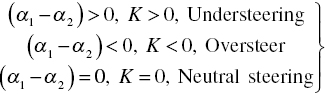

Figure 5.2 Vehicle steady yaw rate gain curves.
5.2.2 Transient Response
First, equations (5.8) and (5.9) can be rewritten as follows:
where ![]() ,
, ![]() ,
, ![]() ,
, ![]() .
.
From equation (5.21), the following can be calculated:

Combining this with equation (5.20), and eliminating β, the differential equation of ![]() can be organized into the following:
can be organized into the following:
where ![]() ,
, ![]() ,
, ![]() ,
, ![]() ,
, ![]() .
.
This is a second-order differential equation of forced vibration, and can be further rewritten as:
where ![]() ,
, ![]() ,
, ![]() ,
, ![]() .
.
When the angle step input is applied to the front wheel, the front wheel angle can be expressed as:
Substituting this last expression into equation (5.23), when t > 0:
Equation (5.24) is a second-order non-homogeneous differential equation with constant coefficients. Its general solution is equal to the sum of a special solution and a general solution of its corresponding homogeneous differential equation. Its special solution is:

The steady state yaw rate is  .
.
The taken Laplace transform is taken from equation (5.23) on both sides getting:

Considering ![]() , then the solution of equation (5.25) has three cases.
, then the solution of equation (5.25) has three cases.
The roots of the characteristic equation are:
![]() A pair of conjugate complex roots
A pair of conjugate complex roots
![]() A double root
A double root
![]() Two different real roots
Two different real roots
The general solution of the homogeneous equation is:
where C, φ, C1, C2, C3, C4 are integration constants, which can be determined by the initial motion conditions.
When ![]() , it means that there is a large damping in the system, and the yaw rate response ωr(t) is monotonically increasing. With the growth of time, ωr approaches the steady state yaw rate. But, after the vehicle exceeds the critical speed, ωr is divergent and tends to infinity, and the vehicle loses stability at this time.
, it means that there is a large damping in the system, and the yaw rate response ωr(t) is monotonically increasing. With the growth of time, ωr approaches the steady state yaw rate. But, after the vehicle exceeds the critical speed, ωr is divergent and tends to infinity, and the vehicle loses stability at this time.
When ![]() , called critical damping, the yaw rate response ωr(t) is also monotonically increasing and approaches to a steady state yaw rate.
, called critical damping, the yaw rate response ωr(t) is also monotonically increasing and approaches to a steady state yaw rate.
When ![]() , called small damping, the yaw rate response ωr(t) is a reduction sine curve which converges to a steady state yaw rate.
, called small damping, the yaw rate response ωr(t) is a reduction sine curve which converges to a steady state yaw rate.
As vehicles usually have small damping, the variation of the yaw rate response when ![]() is the following
is the following

Let ![]() . The initial conditions for the motion are:
. The initial conditions for the motion are:
According to equation (5.9),

Equation (5.25) can also be written as rational fractions:

Comparing equation (5.25) with equation (5.26), the following can be obtained:
Equation (5.25) can be obtained from the Laplace inverse transform:
where:

Equation (5.28) can be further rewritten as:

where:
The time history curves of the yaw rate response are shown in Figure 5.3, in which ξ has a great impact on the yaw rate response.

Figure 5.3 Yaw rate response time history.
The greater the damping ratio ξ, the faster the attenuation of the yaw rate response. When the damping ratio ξ is small, the attenuation of the yaw rate response is slow and the overshoot is large. The following curves in Figure 5.3 show that the yaw rate finally tends to a steady yaw rate ![]() .
.
Generally, the quality evaluation of the transient response comes from the undamped natural frequency ω0, damping ratio ξ, overshoot, and other parameters.
5.2.3 The Frequency Response Characteristics of Yaw Rate
If the vehicle is a linear dynamic system, it has frequency retention. When the input is a sine function, the steady-state output is also a sine function with the same frequency. But the input/output amplitude and phase are different. The ratio of the input/output amplitude is a function of frequency f, called amplitude-frequency characteristics A( f ). The phase difference is also a function of f, called phase-frequency characteristics φ( f). Both of them are named as the frequency response characteristics, and can be represented unified by using the frequency response function H( f ).
5.3 Handling Stability Evaluations
Currently, handling stability is evaluated subjectively and experimentally by most automobile manufacturers.
5.3.1 Subjective Evaluation Contents
The evaluation contents of a vehicle handling stability analysis include static state evaluations and dynamic evaluations; the common evaluation items are depicted in Table 5.1.
Table 5.1 Subjective evaluations of handling stability.
| Static evaluations | Steering wheel | Steering wheel size |
| Adjusting angles of the steering wheel | ||
| Steering in-situ | Slow and even steering force under idle speed | |
| Fast steering force under idle speed | ||
| Dynamic evaluations | Straight-running stability | Uniform speed running on smooth road surface |
| Accelerating running on smooth road surface | ||
| Running with braking on smooth road surface | ||
| Uniform speed running on rough road surface | ||
| Steering portability | Steering force under low-speed cornering | |
| Steering force under high-speed cornering | ||
| Steering wheel rebound force with large lateral acceleration while cornering | ||
| Aligning performance | Aligning performance at low speed | |
| Aligning performance at medium and high speeds | ||
| Steady turn performance(fixed circle driving) | Understeering characteristics | |
| Roll characteristics | ||
| Limited speed of tyre sideslip | ||
| Transient performance | Body roll at high-speed lane change | |
| The steering response to high-speed lane change | ||
| The tyre grip performance of high-speed lane change |
5.3.2 Experimental Evaluation Contents
Currently, Chinese standard QC/T 480–1999 is implemented to evaluate handling stability. The criterion thresholds and evaluation of the handling and stability of a vehicle can be carried out by using six test evaluations, such as steady steering, transient response of the steering wheel angle step input, transient response of the steering wheel angle pulse input, steering aligning performance, steering portability, and snaking tests. Information about the vehicle handling and stability is basically included in the evaluation of these projects. Of course, more companies carry out test evaluations with reference to advanced country standards.
5.4 Four-wheel Steering System and Control[3]
The sideslip angle of the body’s centroid is mainly used to describe the problems of keeping track of the vehicle stability control. Although the centroid sideslip angle can be determined by the lateral and longitudinal forces applied to the vehicle, it is difficult to use the braking or the driving forces to directly control the vehicle lateral forces. Four-wheel steering is an important component of vehicle chassis active control technology, and also an important method of controlling vehicle stability. It can not only reduce the centroid sideslip angle, but also increase the tyre lateral force margin. It has the advantage of easily implementing track keeping and sideslip angle control, and is one of the developing directions of modern automotive technologies.
With the development of four-wheel steering vehicles, their control objectives are being deepened, and the control performance is being improved. In particular, it requires that the system can withstand the impact of vehicle parameter changes and maintain the desired steering characteristics, and also requires that the system still has a good response characteristic when the tyres reach the limit state. Under certain conditions, better control effects can be achieved by adaptive control and robust control. However, as the input values of the steering angle are very small under high lateral acceleration, it is difficult to accurately identify the vehicle real-time response parameters and, subsequently, design an adaptive control system and analyze the system’s stability. In the application process of robust control, its ultimate controller design can be attributed to the solution of linear matrix inequalities, so it cannot be fully inclusive of the nonlinear error caused by the reduced tyre cornering stiffness and may make the control system unstable.
As the vertical and horizontal forces of the tyres and the road adhesion are interdependent and have a nonlinear relationship with the vertical loads, the nonlinear control algorithms should be used for the four-wheel steering. But, the uncertainty of the driving conditions and the environmental changes, robustness and adaptiveness should be required for the system.
Among them, the control algorithms based on neural network theory are effective methods for four-wheel steering nonlinear control. The nonlinear characteristics of the tyre/road contact at high lateral acceleration can be identified by using the neural network model. Through the online correction of the neural network weightings, the system has the adaptive capacity of withstanding vehicle parameter changes and maintaining the desired steering characteristics to accommodate for the nonlinear motion of the vehicles.
Based on the ideas expressed above, the hybrid control system of the yaw rate feedback and adaptive neural network is constructed. Through online correction of the neural network weightings, it has the adaptive capacity when the nonlinear control system is implemented. The virtual prototype model of the four-wheel steering vehicle is also constructed based on the software ADAMS/Car, and the co-simulation analysis in ADAMS and MATLAB environment is studied, so the effectiveness of the hybrid control system is verified.
5.4.1 Control Objectives of the Four-wheel Steering Vehicle
The rear tyre lateral force can be controlled directly and independently by a four-wheel steering vehicle, and the front and rear sideslip angles and lateral forces of the tyres can be changed simultaneously. Thus, the vehicle transient response performances and steering control capability can be improved. The control objectives can be summarized as follows:
- Reducing the sideslip angle at the centroid
- Achieving low speed with good maneuverability, high speed with good stability
- In a certain frequency range, the gain and phase between the lateral acceleration, yaw rate, and steering angles with small changes
- Reducing the phase difference between the lateral acceleration and yaw rate, and their respective phases
- Achieving the desired steering characteristics
- Withstanding the system parameter changes, maintaining the desired steering characteristics
- When the tyres reach the limit state, they still have a good response.
5.4.2 Design of a Four-wheel Steering Control System
5.4.2.1 Yaw Rate Feedback Control of a 2-DOF Linear Model
The simplified 2-DOF linear model of a four-wheel steering vehicle is an important vehicle model that is still used in the various literature, which studies the dynamic characteristics of the four-wheel steering vehicle. Although the yaw rate and centroid sideslip angles determined by the 2-DOF linear vehicle model are only accurate in the linear region of the tyres, it is more stable to the vehicle, and it is relatively easy to grasp the steering characteristics for a driver. The model can be expressed as:

where δf, δr are the steering angles of the front and rear wheels respectively, and the other symbols are the same as before.
Comparing with the feed forward control, feedback control of the four-wheel steering system reduces the external interference more effectively. When the above linear model is used by the rear wheel steering control, the prominent features are the simple calculations and fast response. The control quantity depends on the steering angles of the front wheels and vehicle operating parameters, and it can be expressed as:
where ![]() ,
,  , L is the wheelbase, and a, b are the horizontal distances between the body mass center and the front and rear axles.
5.4.2.2 The Design of a Nonlinear Control System Based on the Neural Network Theory
Based on the feedback control scheme of a 2-DOF linear model, the tyre cornering force is considered to vary linearly with the sideslip angles, without considering the impact of nonlinear factors such as tyres. When the sideslip angles are larger, the error of the linear model is larger. This cannot meet the higher control requirements of modern four-wheel steering vehicles. Based on this, the problem can be solved by using nonlinear control theory. The four-wheel steering control method based on artificial neural network is an effective way which considers the nonlinear dynamic characteristics of the vehicle and tyres. The neural network control system of the four-wheel steering system can be expressed as follows:
In Figure 5.4, y is the system output, including the yaw rate and the sideslip angles, and y* is the reference system input. The network structure 6-10-2 is used in the identification neural network AN1.The six input variables are the yaw rate ωr, centroid sideslip angle β, speed u, lateral acceleration ay, and front, rear wheel steer angles δf and δr. The two output variables are the yaw rate ωr and centroid sideslip angle β. The activation function of the hidden layer and output layer is the bipolar function. Considering the nonlinear effects of the tyres, the variation of the front steering angles with time by using a multi-body dynamic model for sampling needs a variety of modes. The rear steering angles can be a random mode. The calculation of data in each mode is saved as learning samples for later training.
Figure 5.4 The neural network control system of a four-wheel steering vehicle.
The yaw rate feedback control shows that the output of the rear steering angles is related to the yaw rate, vehicle speed, and front steering angle. Therefore, the network structure 4-6-1 is used in the neural controller AN2. The four input variables are the yaw rate ωr, speed u, front steering angle δf, and lateral acceleration ay. The output variable is the rear steering angle δr. The activation function of the hidden layer and output layer is the bipolar function. The output of the rear steering angles is needed for proper gain calculation. Here, comparing with the yaw rate feedback control of a linear 2-DOF model, the input of AN2 has an additional parameter, the lateral acceleration. The purpose is to show the nonlinear characteristics and compensate the linear control error at large lateral acceleration. The offline training of AN1 and AN2 can be used to access weighting coefficients of each layer.
The neural controller AN2 is trained through the back-propagation algorithm. First, the neural identification network AN1 is required to do the error back-propagation. However, in order to facilitate the use of the function call method in MATLAB, the neural network toolbox for training is used, and the system is treated as a complex network. Therefore, AN1 and AN2 are combined into a composite neural network system of a four-wheel steering vehicle system, which is a composite network 4-6-1-10-2. The first layer of the network has 4 neurons, the second layer has 6 neurons, the third layer has only 1 neuron, and the output signals are the rear steering angles. The fourth layer has 10 neurons, and the output layer has 2 neurons. The output signals are the body yaw rate ωr and sideslip angle β. With the exception of the input layer, the activation function of each layer is the bipolar function. Wherein, in addition to receive the steering angle signals of the rear wheel of the second layer, the third layer also accepts the feedback signals of the fourth layer. The four variables of the network are ωr, u, δf, ay, respectively, and the six variables of the second layer are δr, u, ay, δf, ωr, β. The topology of the neural network control system of the four-wheel steering system is shown in Figure 5.5.

Figure 5.5 The topology of the neural network system of a four-wheel steering system.
Excluding the input layer, Figure 5.5 can be viewed as a 4-layer neural network where f1, f2, f3, f4 are the transfer function (activation function) of each layer of the network, respectively. In addition, b1, b2, b3, b4 are the offset (threshold values) of each layer neurons, respectively. Also, IW1,1 is the network weight between the input layer and the first layer, and IW3,1 is the network weight between the input layer and the third layer. The network weight LW1,4 is between the fourth layer and the first layer of the network, LW2,1 is the network weight between the first layer and the second layer, LW3,2 is the network weight between the second layer and the third layer, LW3,4 is the network weight between the fourth layer and the third layer, and LW4,3 is the network weight between the third layer and the fourth layer. TDL is the time-lag, and the current time signal can be delayed several times.
Assuming AN2 has been trained, in order to train AN1, the output error of AN2 is back-propagated to AN1. The error signals shared with the layers of AN1 are used to adjust the weight matrix of the corresponding layer, until the index function of the network performance satisfies the requirements. In training, only the weight matrix of AN2 is modified. The weight matrix of AN1 represents the nonlinear dynamic characteristics of the vehicle and tyres. The trained property of the network object can be set to non-modification by using MATLAB, and the system identification is completely trained before. A network performance index J presented in equation (5.32) is the sum of the squares of the sideslip angle β. Where p is the sample size, i is the order number, and q is the number of the sampling.

5.4.2.3 A Hybrid Control System of the Yaw Rate Feedback and Neural Network
Nonlinear problems can be solved effectively by four-wheel steering neural network control systems. However, when the neural network is trained to be used offline, it is not adaptive. To make the system adaptive, this neural network control system can be trained offline to obtain network weights. After that, using online methods, the system has the adaptive capacity through the online learning correction. In order to facilitate the network with the weights which were adjusted online, the yaw rate feedback control and neural network control are combined. The hybrid control system is shown in Figure 5.6.

Figure 5.6 The four-wheel steering hybrid control system.
The next step is the online correction of AN2 to make the neural network adaptive. Methods are summarized as follows. When the output error between AN1 and the vehicle model exceeds the limit value, the input and output variables of the neural network in this condition are trained as a new sample, and the weight coefficient matrix of AN1 is set immutably. The weight coefficient matrix of AN2 is corrected online, and the correct neural controller is used for control calculations at the next time. Thus, AN1 is adaptive to the changes of the controlled target, and the neural network control system has the function of self-learning/self-tuning while online. It can overcome the various errors caused by parameter variation, not only solving nonlinear problems, but also by making the system adaptive.
The amount of actual control from the hybrid control system is determined by the sum of the output of the feedback controller and neural controller. This reflects the nonlinear compensation from the neural controller to the vehicle yaw rate feedback control, which is based on the linear 2-DOF model. Meanwhile, the effectiveness of the four-wheel steering control system is guaranteed by the feedback controller, and the learning tasks of the neural network are reduced. This makes the workload of the online self-learning/self-tuning reduce, and the nonlinear adaptive control achievable.
5.4.3 Multi-body Dynamics Modeling of a Four-wheel Steering Vehicle
Currently, the virtual prototyping software ADAMS has been widely used for modeling, solving, and visualizating vehicle dynamics technology. But due to functional limitations of the ADAMS software, the CAR module does not include the templates of a rear-wheel steering system. To make the rear wheel section with a steering function, a secondary development is created based on the existing rack and pinion steering templates. The rear-wheel steering subsystem is composed by the MacPherson rear suspension; and then the four-wheel steering vehicle model is assembled. The subsystems include the MacPherson front (rear) suspensions, front (rear) rack and pinion steering systems, braking system, wheels, body and so on.
In the ADAMS/CAR module, the rear-wheel steering angle can be controlled to achieve the four-wheel steering by adjusting the steering-gear angular displacement. Meanwhile, the displacement of the steering-gear angular displacement can be determined by the above control signals of the rear-wheel steering angles. Considering the four-wheel steering has certain requirements for the delay characteristics of the hydraulic system, the large delay of the hydraulic system will have an effect on the control stability of the four-wheel steering. Through theoretical analysis and experimental research into the hydraulic system, the delay characteristics of the hydraulic control system can be treated as the composition of the throttle and pure delay characteristics. To simplify the analysis, ignoring the throttle characteristics delay in the simulation, the pure delay inertia link of the hydraulic system is increased, and the time-lag of the hydraulic system is simulated to make the results more realistic and effective.
In the ADAMS/CAR modules, the topology of the components of each subsystem is defined. The subsystems of the four-wheel steering vehicle are built. Here, the rear-wheel steering subsystem is constructed as follows.
The rear-wheel steering subsystem is composed of the steering wheel, steering shaft, steering column, steering output shaft, steering rack and other components, and is connected with the rear suspension and body through the data communicator. In order to achieve a four-wheel steering control, setting input and output variables are needed for the rear-wheel steering subsystem in the model. Creating a state variable, and make it correspond to the control signals of the rear-wheel steering. The size of this control signal is matched to the steering angle signals of the rear-wheel by the gain link, and the state variable is set to be the input variable by using the Build-controls Toolkit in ADAMS. So, in the co-simulation, through the predefined input and output interface in the co-simulation, the steering-angle control signals calculated by the controller models of SIMULINK can be transferred to the vehicle models in ADAMS as the input values at each simulation step.
After completing the above steps and inputting the vehicle structural parameters, the following dynamic equations can be established:

where M is the generalized mass matrix, QA is the generalized force matrix, Φq is the Jacobian matrix where ![]() , q is the system generalized coordinates, λ is the Lagrange multiplier array, and γ is the right term of the system acceleration equations.
, q is the system generalized coordinates, λ is the Lagrange multiplier array, and γ is the right term of the system acceleration equations.
The kinematic analysis of each subsystem can normally be operated by simulating the multi-body models. The major physical parameters of the vehicle are shown in Table 5.2, and the virtual prototype model is shown in Figure 5.7.
Table 5.2 Main structural parameters of the vehicle.
| Parameter | Value |
| Body mass/kg | 1247.5 |
| Body roll moment of inertia/kg.m2 | 300 |
| Body pitch moment of inertia/kg.m2 | 1067.2 |
| Body yaw moment of inertia/kg.m2 | 1181.8 |
| Front mass/Rear mass/kg | 37.6/43 |
| Wheelbase/mm | 2800 |
| Tread/mm | 1540 (front)/1540 (rear) |
| Body centroid and rear axle distance/mm | 1320 |
| Body centroid height/mm | 450 |
| Caster angle/( |
3 |
| Kingpin inclination/( |
13 |
| Camber/( |
0.5 |
| Toe angle/ ( |
0.1 |

Figure 5.7 Vehicle virtual prototype model.
5.4.4 Simulation Results and Analysis
To validate the correctness and validity of the vehicle model and control strategies, co-simulation and analysis are carried out in this section based on ADAMS and MATLAB. The simulation results are shown in Figure 5.8. In the simulation, the speed is 80 km/h, and the road’s surface adhesive coefficient is 0.8.

Figure 5.8 Simulation results. (a) Steering-wheel angle input. (b) The yaw rate response. (c) The sideslip angle response. (d) The rear wheel angle response. (e) The lateral displacement response.
The simulation results show that, compared with the linear control of the front-wheel steering and four-wheel steering systems, the yaw rate, sideslip angle, and other parameters of the hybrid control system are markedly improved through the rear-wheel angle control of the four-wheel steering system. The handling and stability of the vehicle are effectively improved. The lateral displacement responses show that, when the four-wheel steering system has the same steering-wheel input, the decrease of the lateral displacement and steering sensitivity may affect the vehicle driving performance. Theory analysis and simulation results show that the constructed hybrid control system of the yaw rate feedback and neural network adaptive control of the four-wheel steering vehicle can effectively improve handling, stability, and security. This proves the good effects of the hybrid control algorithm. In addition, the control effects of the four-wheel steering vehicle in different road adhesive coefficients have been studied, and the system performance is improved effectively.
5.5 Electric Power Steering System and Control Strategy
The control strategy of a traditional electric power steering system (EPS) is mainly based on a linear vehicle model of two degrees of freedom. An improved steering portability and aligning performance can be obtained through the design of the control strategy. On a low adhesive road, the linear region and amplitude of the tyre self-aligning torque are obviously decreased. When steering on a low adhesive road at higher speeds, the self-aligning torque generated by the road and tyres will be greatly reduced. The driver tends to turn the steering wheel, and this operation will lead to slip trend and go into a dangerous state. When returning, as the self-aligning torque is not enough to overcome the internal friction of the steer system, the aligning performance is insufficient. This period involves a delay in adjusting the steering which makes the vehicle more difficult to handle, with the possibility of accidents.
The EPS dynamics model is established in this section. The torque values are obtained from the motor current and the torque sensor. Eliminating other factors, the self-aligning torque on the present road is obtained by a mathematical fitting. Meanwhile, the additional self-aligning torque on the ideal road is calculated through the steering wheel angle signals. Combining with the road estimation algorithm, a new EPS control strategy has been designed which includes a power-assisted control by adjusting the current and the aligning control by a time-varying sliding mode.
5.5.1 EPS Model
The EPS model is shown in Figure 5.9.

Figure 5.9 EPS dynamics model.
For convenience, the front wheel and steering mechanism are simplified as the steering shaft, and the dynamics equations are as follows[4,5]:
where θm is the assisting-motor angle; θc is the steering shaft angle; N1 is the transmission ratio of the motor to the steering shaft; N2 is the transmission ratio of the steering shaft to the front wheels; δf is the front-wheel angle; Th is the steering wheel torque; Ts is the value of torque sensor measurement; Ks is the torsion stiffness coefficient; θh is the steering wheel angle; Jh is the steering wheel moment of inertia; Ch is the steering wheel damping coefficient; Ta is the assisting-motor torque; Tr is the steering-torque acting on the steering pinion; JP is the equivalent moment of inertia of the steering shaft; and CP is the equivalent damping coefficient of the steering shaft.
The direct current motor is adopted by the system, then:
where U, I are the voltage and current of the motor, respectively; Lm, R are the inductance and resistance of the motor, respectively; Kb is the counter-electromotive force coefficient of the motor; Ka is the torque coefficient of the motor; Jm is the moment of inertia of the motor; and Cm is the damping coefficient of the motor.
5.5.2 Steering Torque Model of the Steering Pinion
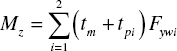
To use the steering torque and assisting-current of the motor, which could be measured to estimate the tyre self-aligning torque and the road adhesive coefficient, it is necessary to make sure that the steering torque Tr of the steering pinion follows the model[6,7]:
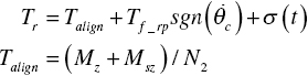
where Talign is the aligning torque equivalent to the steering pinion; Mz is the self-aligning torque of the front-wheel; Msz is the aligning torque caused by gravity; Tf_rp is the friction torque of the steering system; and σ(t) is the interference function related to the road.
In order to ensure the accuracy of the estimation algorithm of the road, the following will analyze the mathematical expression of each torque in equation (5.41).
5.5.2.1 Tyre Self-aligning Torque Model
Ignoring the influence of the vehicle roll factor, the nonlinear vehicle model (front-wheel steering) is used as shown in Figure 5.10, in which ![]() 1, 2, 3, 4 represent the left front, right front, left rear and right rear wheel, respectively.
1, 2, 3, 4 represent the left front, right front, left rear and right rear wheel, respectively.

Figure 5.10 Vehicle model.
The dynamic equations are:
where m, Iz are the vehicle mass and moment of inertia with respect to z-axis, respectively; u, v are the longitudinal and lateral speeds, respectively; Fx, Fy are the longitudinal and lateral forces, respectively; ωr is the yaw rate; a, b are the distance of front, rear axle to the centroid, respectively; and d is the track width.
The decomposition of the contact forces of the tyres and road in the body heading Cartesian coordinate system is shown in Figure 5.11.

Figure 5.11 Tyre and ground forces.
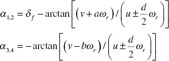
Assuming the steer angles of the left and right wheels are the same; thus, ![]() ,
, ![]() . From the analysis of Figure 5.11, the formula is expressed as follows:
. From the analysis of Figure 5.11, the formula is expressed as follows:

where Fxw, Fyw are the tyre longitudinal and lateral forces, respectively.
Ignoring the effect of the moment of the inertia and air lifting force, then:

where Wi is the vertical load of the tyres; L, h are the wheelbase and vehicle centroid height, respectively; αi is the tyre sideslip angle; g is the acceleration of gravity; and ax, ay are the longitudinal and lateral accelerations of vehicle, respectively.
The nonlinear Dugoff tyre model is used in the simulation. Assuming the cornering stiffness of the left and right tyres is the same and the longitudinal stiffness of the tyres is also the same, the equations can be derived as follows[8]:


where Fxw, Fyw are the tyre longitudinal force and lateral force, respectively; λ is the wheel longitudinal slip ratio; τ is the speed impact factor; Kα, Cs are the tyre cornering stiffness and longitudinal stiffness, respectively; μ is the adhesion coefficient between the tyre and the road; ζ is the tyre dynamic parameter; and ψ (ζ) is the related function of ζ.
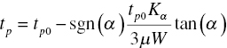
Tyre self-aligning torque results from the tyre lateral force and the offset distance of the tyres. The offset distance of the tyres is the sum of the mechanical offset caused by the kingpin caster and the pneumatic tyre offset. Mechanical offset tm is treated as a certain value, and the pneumatic tyre offset tp is different which is affected by the tyre cornering stiffness, road adhesive coefficient, slip angle, and other factors. Supposing tp0 is the initial value, the expression is given as follows:
Under the condition of the road adhesive coefficient ![]() , the characteristics of the tyre cornering force Fy and self-aligning torque Mz changing with the tyre slip angle are as shown in Figure 5.12. The figure shows that, with the increase of the tyre slip angle, the self-aligning torque reaches saturation earlier than the cornering force. After reaching the peak, the tyre self-aligning torque decreases dramatically. Generally, the region of the self-aligning torque before the peak is called the linear region. With the decrease of the road adhesive coefficient, the linear region of the tyre self-aligning torque and the amplitude will decrease.
, the characteristics of the tyre cornering force Fy and self-aligning torque Mz changing with the tyre slip angle are as shown in Figure 5.12. The figure shows that, with the increase of the tyre slip angle, the self-aligning torque reaches saturation earlier than the cornering force. After reaching the peak, the tyre self-aligning torque decreases dramatically. Generally, the region of the self-aligning torque before the peak is called the linear region. With the decrease of the road adhesive coefficient, the linear region of the tyre self-aligning torque and the amplitude will decrease.

Figure 5.12 The characteristics of tyre lateral force and self-aligning torque.
At the same time, at certain speeds, such as at 36 km/h, with the same steering-wheel angle control, if the road adhesive coefficient is low, the linear region of the tyre self-aligning torque and the amplitude will decrease. The simulation results are shown in Figure 5.13.

Figure 5.13 The tyre self-aligning torque under different adhesive road conditions.
5.5.2.2 Model of Aligning Torque Caused by Gravity
The other part of the aligning torque is generated by the load of the front axle of the vehicle and the geometry of the front suspension. It can be described as[9]:
where Dn, φ are the kingpin offset and inclination angle, respectively; and Wf is the front axle load.
5.5.2.3 The Internal Friction of the Steering System and Road Disturbance
Under steering in in-situ conditions, the driver releases the steering-wheel, then it returns to the center position a little but cannot reach the center perfectly. The values of torque sensor will slowly recover to the initial values. The reason is due to internal friction torque Tf_rp of the steering system. The results measured by the experiments are shown in Figure 5.14.

Figure 5.14 The internal friction torque of the steering system.
In addition, the friction torque of the road and tyres can be regarded as the road related interference function σ(t) in the process of vehicle driving.
5.5.3 The Estimation Algorithm of the Road Adhesion Coefficient
At present, the error generated by a variety of estimation algorithms of the road adhesive coefficient is relatively large, and the cost of accurately identifying the road’s information is very high. With the commercial application of a torque/angle integrating sensor, it can provide the position and torque information of the steering wheel better than traditional torque sensors, and is convenient for the development of the aligning control algorithm. Combined with the estimation algorithm of the road adhesive coefficient, the class of the identified adhesive coefficients can be divided into high, medium, and low, namely, μh, μm, and μl, as follows:
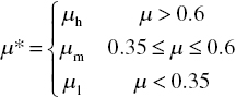
where μ* is the estimation value of the road adhesive coefficient.
Assuming the adhesive coefficient ![]() and the simulation speed is 36km/h, when the vehicle is driving in steady state the maximum self-aligning torque of the front wheel is the additional self-aligning torque Ms0.
and the simulation speed is 36km/h, when the vehicle is driving in steady state the maximum self-aligning torque of the front wheel is the additional self-aligning torque Ms0.
The motor’s current is measured by the current sensor and combining equations (5.39)–(5.40), where the assisting-motor torque Ta is gained. By adding the steering torque and eliminating the aligning torque caused by gravity, the system’s friction and other disturbances, such as the estimation values of the self-aligning torque can be obtained as shown in Figure 5.15. Then, through calculating ![]() and estimating the adhesive coefficient combined with Figure 5.15, the estimation values μ* can be calculated. The estimation algorithm flow is shown in Figure 5.16.
and estimating the adhesive coefficient combined with Figure 5.15, the estimation values μ* can be calculated. The estimation algorithm flow is shown in Figure 5.16.

Figure 5.15 The estimation results of the self-aligning torque.

Figure 5.16 The estimation algorithm of the road adhesive coefficient.
5.5.4 Design of the Control Strategy
In the literature[4–5], there is a representative method of the traditional EPS control strategy. Generally, the motor reference current Iref is determined by the power-assisted curves or look-up table method combined with the speed and torque sensor signals, and then the power-assisted or aligning control will be achieved. But the slippery road is not considered; that is, the influence on the vehicle handling performance on the low adhesive road is not considered. In the actual steering, the driver continues to adjust the steering and aligning movement, so the power-assisted and aligning control strategies are designed respectively.
In the steering process, the motor current is reduced appropriately; thus, the power-assisted torque is reduced and the steering torque of the driver is increased, so the power-assisted current Iassist is designed as:

where Irev is the correction current, and Kμ is the current correction factor.
Under low adhesive conditions, when in the aligning process the self-aligning torque is not enough to overcome the internal friction of the steering system where the aligning ability is inadequate. The sliding mode controller can overcome the aligning torque changes in different adhesive coefficients and reduce the effect caused by friction and other uncertain factors on the system. Its application to the aligning control can obtain good results. However, the discontinuous switching of the traditional sliding mode controller will cause chattering, which will give a worse hand feel. Therefore, the control method can effectively eliminate the chattering by reducing the switching gain. The time-varying sliding mode control method is able to make the system state in the sliding mode surface within the setting time. Therefore, the robustness of the approaching mode is strengthened, and the approaching mode of the traditional sliding mode control is eliminated.
Let,
where θd is the desired steering-wheel angle, and e is the error.
From the simulation of three kinds of time-varying sliding surfaces in the literature[10], the method of variable slope sliding surface is better than the other two methods, and can be expressed as:


where A, B, λ, tf are constants and ![]() ,
, ![]() ; e0,
; e0, ![]() are the values of e and
are the values of e and ![]() at t = 0, respectively.
at t = 0, respectively.
The estimation of ![]() of the steering torque Tr, due to the moment of inertia Jm and the damping coefficient Cm of the motor are small, and can be neglected here. Therefore, equation (5.38) becomes:
of the steering torque Tr, due to the moment of inertia Jm and the damping coefficient Cm of the motor are small, and can be neglected here. Therefore, equation (5.38) becomes:
and,

where ΔTr is the uncertain value of Tr; ΔC, ΔJ are the uncertain values of CP and JP; C0, J0 are the certain values of CP and JP; ΔTmax, ΔCmaxare the upper limit values of ΔTr and ΔC; and ΔJmax, ΔJmin are the upper and lower limit values of ΔJ.
To solve the derivative of variable s in equation (5.56), we get:

From (5.59), the equivalent control law is as follows:

When aligning, the motor current Ireturn is designed as:

The Lyapunov function is defined as:
By the Lyapunov stability theorem, when ![]() (
(![]() ), the system is stable, thus,
), the system is stable, thus,
where:

Obviously, f(ΔJ, ΔTr) is bounded. When ![]() ,
, ![]() ,
, ![]() ,
, ![]() , the Lyapunov stability criterion is satisfied.
, the Lyapunov stability criterion is satisfied.
In order to reduce the system chattering, the following saturation function  is used to instead of the symbol function sgn(s) in equation (5.61). And thus:

where ε is the thickness of the boundary layer.
Figure 5.17 illustrates the overall system control strategy.

Figure 5.17 EPS control strategy.
5.5.5 Simulation and Analysis
The structure parameters of a vehicle in simulation are shown in reference[9]. With the road adhesive coefficients μ = 0.5 and 0.3, at the speed of 36 km/h, using the same control method from the EPS described above, the steering torque and aligning performance are simulated. When the adhesive coefficient μ = 1, the performance of the designed controller in this section is similar to the performance of the traditional controller, so the latter will not be discussed.
5.5.5.1 Steering Torque
Figure 5.18(a) shows the simulation results when μ is 0.5 (in the figure, the traditional control strategy is presented in references[4] and[5]). In the steering process, the new control strategy presented in this section does not increase the steering torque. When the steering wheel returns, the steering torque is increased slightly (about 0.2 Nm). The motor provides a smaller aligning torque to improve the aligning performance.

Figure 5.18 The simulation results of the steering torque. (a) Steering torque (μ = 0.5). (b) Steering torque (μ = 0.3).
Figure 5.18(b) shows the simulation results when μ is 0.3. In the steering process, the steering torque (about0.5 Nm) is slightly increased by the new control strategy. After the steering angles increase to a certain level, the steering torque is obviously reduced, so it can alert the driver that it is on a low adhesive road for suitable hand-feeling. Meanwhile, when the steering wheel returns, the steering torque is greatly increased (about 1.2 Nm), and a larger aligning torque is provided by the motor to improve the aligning performance.
5.5.5.2 Aligning Performance
Figure 5.19(a) shows the simulation results when μ is 0.5. In the aligning process, a large aligning torque can be provided by the motor to improve the aligning performance. This can be seen from the residual steering wheel angle shown in the simulation graph. Figure 5.19 shows that the residual steering wheel angle is close to ![]() when the traditional control strategy in reference[5] is used, and the aligning process needs a longer period of time. However, a shorter time is expended for the aligning process by using the new control strategy, remaining with a steering wheel angle of about
when the traditional control strategy in reference[5] is used, and the aligning process needs a longer period of time. However, a shorter time is expended for the aligning process by using the new control strategy, remaining with a steering wheel angle of about ![]() . Therefore, the aligning performance is improved.
. Therefore, the aligning performance is improved.
Figure 5.19 The simulation results of the aligning performance. (a) Aligning performance (μ = 0.5). (b) Aligning performance (μ = 0.3).
Figure 5.19(b) shows the simulation results when μ is 0.3. The figure shows that the residual steering wheel angle is close to ![]() and the aligning process needs a longer period of time by using the traditional control strategy. However, using the new control strategy, a shorter time is expended for the aligning process, and the steering angle is slightly reduced.
and the aligning process needs a longer period of time by using the traditional control strategy. However, using the new control strategy, a shorter time is expended for the aligning process, and the steering angle is slightly reduced.
5.5.6 Experimental Study
To verify the effectiveness of the proposed control strategy, a hardware-in-loop experimental study is carried out using LabVIEW software and a self-developed EPS test system. The experimental configuration is shown in Figure 5.20.

Figure 5.20 Experimental configuration of the developed EPS hardware-in-loop system.
Under the condition of a traditional low adhesive coefficient μ = 0.3, the test data are taken for analysis. The steering torque test results are shown in Figure 5.21(a). The figure shows that, compared with the simulation results in Figure 5.18(b), although the amplitudes between the test and simulation results have little difference (about 1 Nm), the variation trend of the steering torque with the steering wheel angle is consistent.

Figure 5.21 Experimental results. (a) Steering torque (μ = 0.3). (b) Aligning performance (μ = 0.3).
Figure 5.21(b) shows the aligning test results: compared with the simulation results in Figure 5.19(b), the test results are basically consistent with the simulation results. Using the traditional control strategy, the residual steering wheel angle is more than ![]() , and the aligning needs a longer period of time. However, using the new control strategy, a shorter time is expended for the aligning control, and the steering wheel slowly reaches the middle position. From a practical point of view, this is in a rational range.
, and the aligning needs a longer period of time. However, using the new control strategy, a shorter time is expended for the aligning control, and the steering wheel slowly reaches the middle position. From a practical point of view, this is in a rational range.
5.6 Automatic Lane Keeping System[11]
Lane keeping systems based on visual navigation include two key technologies: vehicle lateral control and lane detection. In recent years, in-depth research has been conducted by many scholars in this field. In the lateral control area, the nearest point between the vehicle and path is treated as the tracking point by some scholars, and the adaptive PID control and fuzzy preview control methods are designed. The nearest point to the vehicle is chosen as the tracking target, so there is no predictability about the road ahead. Furthermore, the fuzzy rules are difficult to establish, and the control effect is not good enough. In addition, the optimal controller of the autonomous navigation has been designed by some scholars based on the kinematics models, and a better control effect is achieved at low speeds. With the increase of speed, the gap between the kinematics models and the actual vehicle models grows. Therefore, this method is inapplicable to road tracking control of high-speed driving vehicles.
Based on the “preview following theory” for directional control of a vehicle, better path tracking can be achieved. Vehicle lateral control is affected greatly by the selection of the preview points. Under different road curvatures and longitudinal speeds, control effects of the same preview distance have great differences. In order to reduce the effect of the road curvature and preview distance on the lateral control and improve the control precision, a lateral control strategy is presented. This is used to plan a dynamic virtual path between the vehicle and preview points in real time, and produce a desired yaw rate based on the virtual path. Simulation and experimental results show that the proposed lateral control algorithm is valid.
5.6.1 Control System Design
The architecture of the lateral control system is shown in Figure 5.22. In the figure, according to the relative position of the vehicle preview points and vehicle state information from the coordinate transformation, the desired yaw rate as the input of the tracking controller can be produced by the desired yaw rate generator. Based on the nonlinear vehicle dynamics models and the desired yaw rate, the desired vehicle state can be tracked by the yaw rate tracking controller, and the target path is achieved smoothly.

Figure 5.22 The architecture of the control system.
5.6.2 Desired Yaw Rate Generation
At a certain moment, Xc, Yc are the position coordinates of the vehicle centroid in the global geodetic coordinate system (Figure 5.23), and φc is the angle between the vehicle longitudinal axis and the horizontal axis. The vehicle kinematics equations are described as follows:

Figure 5.23 Coordinate system conversion of the vehicle.
where v1is the velocity, and β is the centroid sideslip angle.
Here, the sideslip angle in the left front is defined as positive, and the sideslip angle in the right front is defined as negative. By equations (5.65), (5.66), (5.67), we see that the motion position of a vehicle is determined by the yaw rate, centroid velocity, and sideslip angle. Because the centroid velocity is a vector, and it already contains the sideslip angle information, the motion position of a vehicle is determined by the changes of the yaw rate and centroid velocity. Thus, according to the changes of the centroid velocity, the motion position of a vehicle can be determined by controlling the yaw rate. First, based on the local coordinate system, the path planning is carried out between the vehicle and the preview points. Second, based on the path planning, the yaw rate generator is designed, and the desired yaw rate is treated as the target parameters of the lateral control.
5.6.2.1 Coordinate Transformation
The coordinate transformation of a vehicle is shown in Figure 5.23. In the geodetic coordinate system XOY, Xp and Yp are the coordinates of a point Op located on the road in front of the vehicle preview, and φp is the angle between the tangent direction and transverse coordinate. In the global coordinate system, the relative position between the vehicle and preview point is (Xp, Yp, φp), and now it can be transformed into the relative position (xe, ye, φe) in the local coordinate system of the vehicle.
According to the geometric relation in Figure 5.23, the relative position of the vehicle and preview point Op in the local coordinate system (Xc, Oc, Yc), can be expressed as:

where xe is the preview distance; ye is the lateral deviation between the preview point and the vehicle in the vehicle coordinate system; and φe is the directional deviation between the preview point and the vehicle in the same coordinate system.
5.6.2.2 Path Planning
In the local coordinate system (Xc, Oc, Yc), a virtual path is constructed between the vehicle centroid and preview points in real time, as shown in Figure 5.23. Considering that the sideslip angle is relatively small, the direction of the actual speed at the centroid is supposed to be consistent with the vehicle longitudinal direction.
Assuming the equation of path planning is described as follows:
The known conditions of virtual path are constructed:

where ρ is the curvature of driving path; A, B C, D are the coefficients of the planning path equation.
Combining equations (5.69)~(5.73), the planning curve equation is obtained as:

Obviously, when a vehicle is in the center of the lane and the driving direction is consistent with the tangent direction of the current path, the planning virtual path is the road equation of fitting the target lane central line. If several discrete preview points or a planning curve based on the curvature information at the preview points are selected, the curve in the preview points is more approximate to the actual road. Simulation and experiment results show that practical requirements can be met completely by using one preview point to plan a path. Here, one preview point is adopted to plan a virtual path.
5.6.2.3 Design of a Desired Yaw Rate Generator
It is assumed that a vehicle tracks a path smoothly and without deviation. The path equation y(x) is known, the position of the vehicle centroid at the curve is (x, y), and the velocity is v1. The direction of the velocity and driving curvature are consistent with the point which denotes the position of vehicle at the current curve. When the trajectory of the vehicle is a curve equation, the definition of the corresponding yaw rate is ωd. The changing rate with time of the corresponding yaw rate, ![]() , is studied.
, is studied.
Curvature ρ is:

Changing rate of curvature ρ with time is:

where Sd is the vehicle driving distance. Because driving curvature and road curvature are consistent, then the corresponding yaw rate ωd is:
Combining equations (5.75)~(5.77), the changing rate of ωd with the time is obtained:

In the local coordinate system (Xc, Oc, Yc), the virtual path of the real-time planning equation (5.74) is substituted into equation (5.78), and the values at the origin position Oc are taken in the local coordinate system. At the current moment, when the vehicle approaches the target path along the virtual path, the corresponding changing rate of yaw rate ωd is:

The changing rate of yaw rate shown above represents the changing trend of the yaw rate when a vehicle is approaching the target path with the current speed at this time. It is relevant with the current speed, acceleration, yaw rate, and position preview point. The desired yaw rate can be expressed by the following equation:
where ς is the scale factor associated with the control interval time, ωrr is the desired yaw rate, and ωr is the current yaw rate.
5.6.3 Desired Yaw Rate Tracking Control
In the simulation, consider that the front wheel of a rear-wheel drive vehicle has small longitudinal forces. For brevity, the longitudinal forces of the front wheel can be ignored, and the longitudinal forces of both sides of the rear wheels are equal. Therefore, the yaw moment acting on the vehicle is offered by the wheels’ lateral forces. Supposing the yaw moment is Mz, and according to the nonlinear vehicle dynamics models in[11], it can be shown that:
Generally, the front wheel angle is small, and thus ![]() ,
, ![]() is set, thereby equation (5.81) can be rewritten as:
is set, thereby equation (5.81) can be rewritten as:
In equation (5.82), ΔM is the additional torque which is the un-modeled part as the front wheel longitudinal forces are ignored, and the vehicle models are simplified; thus, they can be viewed as the system interference terms.
Taking the tyre model into the above equation, that is:

where ffl and ffr are the coefficients associated with the maximum road adhesion[11]. T is a simple expression of the rest of the items. To reduce the effect of the system with the unmodeled parts and the parameter uncertainty and improve the system’s robustness, a sliding mode controller is designed to track the desired yaw rate. The sliding switching surface is defined as:
where ωrr is the desired yaw rate, and ωr is the current yaw rate. The derivation of the sliding surface is:
Let the sliding surface close to zero follow an exponential rate, thus, the output of the sliding mode controller is:
The first term δfequ is an equivalent output of the sliding mode control. The second term ensures that, when the system is not in the sliding surface, the system is close to the ideal sliding surface, that is, ![]() . The Lyapunov function is described as:
. The Lyapunov function is described as:
Then, ![]() ,
, ![]() ,
, ![]() . It can be proven that:
. It can be proven that:
If ,
, ![]() , then
, then ![]() .
.
So, the Lyapunov stability criterion is satisfied. Thus, the controller output is:

To weaken the chattering occurring around the sliding surface, the following saturation function  is used instead of sign function sgn(s).

where ε is the thickness of the boundary layer.
5.6.4 Simulation and Analysis
In the MATLAB/Simmulink simulation environment, in order to verify the effectiveness of the proposed algorithm, vehicle models are established and the control algorithm is simulated. Some vehicle parameters are shown in Table 5.3. Supposing that the road is formed by five curves as the simulation path, the simulation results of the lane keeping are compared with the position error feedback control method (shown in reference[12]) and the method proposed in this section. The longitudinal speed is 25 m/s, sampling time t and scale factor ς in equation (5.80) are 0.01.
Table 5.3 Some system parameters.
| Parameter | Value |
| Vehicle mass m/kg | 1704 |
| Vehicle moment of inertia about z-axis IZ/kgm2 | 3048 |
| Distance between centroid and front, rear axis (a, b)/m | 1.015, 1.675 |
| Front and rear wheel track d/m | 1.535 |
|
Front and rear cornering stiffness Kyij/(N/rad) Front and rear longitudinal stiffness K xij /(kN/m) |
−105850, −79030 650,600 |
| Centroid height h/m | 0.542 |
| Tyre rolling radius re/m | 0.25 |
| Preview distance xe/m | 16 |
The simulation results are shown in Figure 5.24.


Figure 5.24 Simulation results. (a) Comparison of tracking trajectory. (b) Comparison of local enlarged trajectory. (c) Comparison of yaw rate, direction deviation, and distance deviation.
From the tracking error curves, compared with the deviation feedback control, the tracking desired yaw rate control has a high accuracy for lane keeping. Also, it can be seen from the tracking error curves that when a vehicle tracks a large curvature, the tracking error can’t get close to zero using the position deviation feedback control. This is because even if the deviation between the vehicle and the preview point is small, the deviation between the vehicle and the nearest point is still large. The control method of the tracking desired yaw rate can track the target path smoothly on any road and has better adaptability.
5.6.5 Experimental Verification
5.6.5.1 Lane Recognition
Lane recognition includes five parts, i.e., Gaussian smoothing filter, lane edge detection, Hough detection of a straight line, vanishing point search, and extraction of the left–right lane lines.
The characteristics of the gray-scale jumping are formed by the lane edge points and other points near the same row of the lane line. The points are generally not less than the width of the lane line, i.e., not less than or substantially equal to the number of pixels of the lane line. Therefore, if the edge points satisfy the width of the lane line, then they can be treated as edge points. The results of the fuzzy edge detection are shown in Figure 5.25(d). It can be seen that, compared with the common edge detection algorithm, the noise can be effectively suppressed by this algorithm.

Figure 5.25 Comparison of fuzzy edge detection. (a) Sobel operator. (b) Prewitt operator. (c) Canny operator. (d) Edge detection.
The direction angles of the edge points are calculated, and the edge points which do not accord with the feature of the direction angles on the left and right lane lines are filtered. The numbers of edge points which are gathered at the vanishing points in different directions are ranked. Then, the parameter information of the straight lines focused on the vanishing points in different directions is available. According to the relative distance between lane lines, the detected lines are classified and extracted. Then the specific distribution locations of the lane lines are obtained. Meanwhile, optimizing the parameters of the lane lines, further information about the deviation parameters of a vehicle and road, and the curvature, is obtained[13]. Figure 5.26 shows some results of lane detection under typical roads.

Figure 5.26 Detection results on different roads. (a) Character interference. (b) Sign interference. (c) Heavy rain. (d) Road of large curvature.
5.6.5.2 Experimental System
As shown in Figure 5.27, the original vehicle steering system is modified and it has an automatic steering function. The experimental system includes the road image collection, vehicle state collection, host and slave computer control, and monitoring systems.

Figure 5.27 Schematic layouts of the experimental system.
As a host computer, LabVIEW PXI8196 is responsible for collecting the signals of the vehicle-mounted sensors, such as the steering wheel angle, yaw rate, lateral acceleration, longitudinal velocity, and road images. The image acquisition card PXI-1411 is responsible for collecting road images from the CCD. Meanwhile, lane recognition and lateral control algorithms are performed in the host computer. The lane recognition module will calculate the relative positions of the vehicle preview points as an input of the lateral control module. As the slave computer, DSP2812 receives control instructions, and converts the instructions into a PWM pulse to control the steering motor to achieve the front-wheel steering. A PC monitors the signals about the vehicle-mounted sensors and the relative positions of the vehicle and the road.
Figure 5.28 shows the interface of the experimental system. Through the real-time display of the lane detection results and motion status signals of a vehicle in the front-end interface, the results of the vehicle lateral motion in different stages are tracked and detected. The lane detection and vehicle control algorithms can be updated and improved in real-time.

Figure 5.28 Test platform of the driver lateral assistance system based on vision.
5.6.5.3 Test Results and Analysis
Two methods of position deviation feedback and tracking desired yaw rate are used for the road tests. A large curved lane and a straight lane are selected as the test roads in order to compare the results.
Experimental results of two control methods are shown in Tables 5.4 and 5.5. It is clear from the tables that, when using the method of position deviation feedback to track the curved lane, the deviation is significantly increased than with the straight lane. When using the method of tracking desired yaw rate to track different lanes, the deviation is small. This indicates that the latter is less affected by the change of the road curvature.
Table 5.4 Distance deviation (straight lane).
|
Longitudinal speed u/(m/s) |
Mean μ/m | Deviation σ2/m2 | ||
| Position deviation feedback method | Desired yaw rate method | Position deviation feedback method | Desired yaw rate method | |
| 2 | 0.0757 | 0.0273 | 0.0338 | 0.0061 |
| 6 | 0.1993 | 0.0329 | 0.0728 | 0.0124 |
| 10 | 0.4713 | 0.0466 | 0.1375 | 0.0327 |
Table 5.5 Distance deviation (curved lane).
| Longitudinal speed u/(m/s) | Mean μ/m | Deviation σ2/m2 | ||
| Position deviation feedback method | Desired yaw rate method | Position deviation feedback method | Desired yaw rate method | |
| 2 | 0.0934 | 0.0382 | 0.0364 | 0.0082 |
| 6 | 0.2965 | 0.0590 | 0.0843 | 0.0216 |
| 10 | 0.6578 | 0.0806 | 0.1995 | 0.0508 |
When tracking the curved lane at low speeds by using the tracking desired yaw rate, the steady-state deviation is very small, about 0.03 m. When the position deviation feedback is used, there is a large lateral steady-state deviation, about 0.08 m. When the road curvature is large, even if the deviation between a vehicle and a preview point is in a smaller range, the deviation of the vehicle and the nearest point in the road center is still large. As shown in Figure 5.29, the results are consistent with the conclusions of the previous simulations.

Figure 5.29 Test results of curved lane keeping. (a) Position deviation feedback control. (b) Desired yaw rate control.
It also can be seen that the deviation of two control methods increases when the speed increases because, even if the lane recognition can basically meet the real-time requirements, the response lag of the steering motor still exists. Even so, the lateral deviation of the lane-keeping system by the proposed method is always less than the deviation of the feedback control. When the longitudinal speed is 10 m/s, the maximum lateral deviation is only 0.08 m. Table 5.6 shows that by using the method of tracking desired yaw rate, the percentage of deviation mean with the speed increasing is less than the position deviation feedback method. This indicates that the desired yaw rate method is less affected by the speed and has higher robustness.
Table 5.6 Percentage of deviation mean with speed increasing (%)
| Type | Position deviation feedback method |
Desired yaw rate method |
| Straight lane | 40.82 | 5.13 |
| Curved lane | 54.36 | 13.61 |
References
- [1] Yu Z S. Automobile Theory. Beijing: China Machine Press, 2009.
- [2] Yu F, Lin Y. Vehicle System Dynamics. Beijing: China Machine Press, 2005.
- [3] Song Y. Study on the control of vehicle stability system and four-wheel steering system and integrated system. Ph.D. Dissertation, Hefei, Hefei University of Technology, 2012.
- [4] Wang Q D, Yang X J, Chen W W, et al. Modeling and simulation of electric power steering system. Transactions of the Chinese Society of Agricultural Machinery, 2004, 35(5): 1–4.
- [5] Zhao L F, Chen W W, Qin M H, et al. Electric power steering application based on aligning and steering performance, Journal of Mechanical Engineering, 2009, 45(6): 181–187.
- [6] Man H L, Seung K H, Ju Y C. Improvement of the steering feel of an electric power steering system by torque map modification. Journal of Mechanical Science and Technology, 2005, 19(3): 792–801.
- [7] Yasui Y, Tanaka W, Muragishi Y, et al. Estimation of Lateral Grip Margin Based on Self-aligning Torque for Vehicle Dynamics Enhancement. SAE Paper 2004-01-1070, 2004.
- [8] Dugoff H, Fancher P S. An Analysis of Tyre Traction Properties and Their Influence on Vehicle Dynamic Performance, SAE Paper 700377, 1970.
- [9] Zhao L F, Chen W W, Liu G. Modeling and verifying of EPS at all operating conditions. Transactions of The Chinese Society of Agricultural Machinery, 2009, 40(10): 1–7.
- [10] Jin Y Q, Liu X D, Qiu W, et al. Time-varying sliding mode controls in rigid spacecraft attitude tracking. Chinese Journal of Aeronautics, 2008, 21: 352–360.
- [11] Wang J E, Chen W W. Vision guided intelligent vehicle lateral control based on desired yaw rate. Journal of Mechanical Engineering, 2012, 48(4): 108–115.
- [12] Wang J M, Steiber J, et al. Autonomous ground vehicle control system for high-speed and safe operation. American Control Conference, 2008: 218–223.
- [13] Zhou Y. Several Key Problem Research of the Intelligent Vehicle. Ph.D. Dissertation, Shanghai Jiao Tong University, 2007.