
3
Longitudinal Vehicle Dynamics and Control
3.1 Longitudinal Vehicle Dynamics Equations
3.1.1 Longitudinal Force Analysis
The dynamics problems along the x-axis in a vehicle coordinate system are called the longitudinal dynamics problems. The characteristics of vehicle acceleration and deceleration are the main research topics, and these two states of motion correspond to, respectively, the traction and braking of the vehicle.
3.1.1.1 Traction
In the case of traction, the force on a car pointing to the positive direction of the x-axis is the longitudinal force produced by the interaction between the driving wheels and the road, which is represented by Fx.
When the tyre is on a high adhesion road, the longitudinal force Fx is equal to the force of traction Ft.

where Tt is the torque transmitted to the driving wheels, Te is the engine torque, ig is the transmission ratio, i0 is the main gear ratio, ηt is the driveline efficiency, and r0 is the driving wheel radius.
When a tyre is running on a poor adhesion road, the longitudinal force Fx is equal to the tyre longitudinal force, which is actually provided by the ground. It can be calculated through the tyre longitudinal force and slip ratio curve, or through tyre models when the tyre motion status is given. The longitudinal slip ratio has a linear relationship with the tyre longitudinal force when the ratio is small; the scale factor is called the longitudinal tyre stiffness[1].
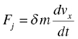
The forces acting on a car driving uphill are shown in Figure 3.1, The longitudinal forces along the negative x-axis direction, the driving resistance, includes the rolling resistance Ff (the sum of the front rolling resistance Fff and the rear rolling resistance Ffr), aerodynamic drag force Fw, ramp resistance Fi, and the inertial resistance. It should be noted that when the car is accelerating the inertial moment of some rotating masses which include the rotating elements of the engine, driveline, and tyre contribute to the driving resistance. For convenience’s sake, the rotating masses are converted to an equivalent translation mass, and only one expression used to denote the inertial resistance. The symbol Fj normally donates inertial resistance.

Figure 3.1 Forces of the uphill accelerating conditions.
3.1.1.2 Braking
When a car brakes while driving uphill, the longitudinal forces along the positive x-axis direction are the inertial forces which are generated by the vehicle deceleration. The forces along the negative x-axis direction include the tyre longitudinal forces, rolling resistance, aerodynamic drag force, and ramp resistance. The tyre longitudinal force is less than the brake force; it is calculated in the same way as in the traction force.
3.1.2 Longitudinal Vehicle Dynamics Equation
To establish the longitudinal vehicle dynamics equation, the status of two movements should be considered: traction and braking. This section focuses on establishing the longitudinal vehicle dynamics equation when the vehicle is in traction.
3.1.2.1 Dynamics Equation
Moving uphill, if the driving force is greater than the sum of the rolling resistance, aerodynamic drag force, and ramp resistance, the excess part of the driving force can be used to accelerate the vehicle.
The dynamics equation is
Equation (3.2) has some advantages in vehicle dynamics analysis but, when studying longitudinal dynamics control problems, a more accurate model is needed which includes the model of the engine, transmission, and tyre.
Taking the Acceleration Slip Regulation control (ASR) as an example, a longitudinal dynamics model can be established in the following way. The static torque of the engine is converted to the dynamic torque to the transmission after a first-order delay, and the transmission model calculates the half axle torque and rotational speed of the driving wheels. The normal force model calculates the normal load on each tyre. The tyre model takes the transmission model and the output from other modelst as its input, calculating the longitudinal velocity, longitudinal acceleration, and other parameters, which are fed back to the transmission model, the normal force model, and the tyre model. Each model will be described in subsequent chapters, and the longitudinal vehicle dynamics model is given here.
3.1.2.2 General Vehicle Longitudinal Dynamics Equation
When a car drives uphill, during both traction and braking, the vehicle longitudinal dynamics equation can be expressed by one equation:
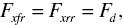
where Fxf is the sum of the longitudinal forces of the front wheels, Fxr is the sum of the longitudinal forces of the rear wheels. The method of calculating these two forces has already been discussed.
The directions of the longitudinal forces are different in traction and braking, the signs of which are indicated in the tyre models.
When braking, all the forces affecting vehicle motion are in the same direction. Compared with the longitudinal tyre force, rolling resistance, aerodynamic drag force, and inertia moment of a rotating mass generated by the car’s deceleration which are much smaller, and can be ignored when establishing the equation.
3.2 Driving Resistance
A vehicle accelerating uphill is in a typical longitudinal running condition. The resistances acting on the vehicle include the tyre rolling resistance, the aerodynamic drag, the ramp resistance, and the acceleration resistance. The tyre rolling resistance has been described in Section 2.2.2. Three other resistances are discussed here.
3.2.1 Aerodynamic Drag
The aerodynamic drag Fw is the component of the air drag force acting on the vehicle along the running direction when the vehicle moves in a straight line. It is made up of pressure resistance and frictional resistance. The pressure resistance is the component of the resultant normal air force acting on the vehicle surface along the running direction. The air, which has a certain viscosity as other fluids, produces friction between air micelles and the vehicle surface as it flows through it; the friction forms the resistance, and its component force along the running direction is called the frictional resistance.
Pressure drag is composed of the shape drag, disturbance drag, internal circulation drag, and induced drag. When a vehicle is moving, air flows through the vehicle surface generating eddy flows in the area where the air velocity changes sharply, building negative pressure in the back and positive pressure in the front. This part of pressure drag caused by eddy flows is related to the shape of the body, so it is called the shape drag, and it accounts for about 58% of the total drag. Disturbance drag is caused by projecting parts of the vehicle body, such as the rearview mirrors, door handles, and projecting parts below the chassis, and it accounts for about 14% of the total drag. Internal circulation drag refers to the resistance caused by air flowing through the inside of the vehicle body, for the purposes of engine cooling, passenger compartment ventilation, and airconditioning. It accounts for 12% of the total drag. When air flows through the asymmetric upper and lower surfaces, it creates a lift force which is perpendicular to the direction of the air velocity, whose component force along the running direction is called the induced drag, which comprises about 7% of the total drag[2]. The aerodynamic drag force is expressed as follows:
where CD is the aerodynamic drag coefficient, ρ is the mass density of air (normally ![]() ), A is the frontal area of the vehicle, vr is the relative velocity of the vehicle where there is no wind condition.
), A is the frontal area of the vehicle, vr is the relative velocity of the vehicle where there is no wind condition.
Considering the car moving in windless conditions, if va (km/h) is used to denote the running speed and A (m2) for the frontal area of the car, the air drag Fw (N) can be expressed as

3.2.2 Ramp Resistance
When moving uphill, the component of a vehicle gravity force along the ramp is called the ramp resistance Fi,
where G is the gravity of vehicle, m is the vehicle mass, g is the acceleration of gravity, and α is the slope angle.
When going up the slope, the component of the vehicle gravity force perpendicular to the ramp is mg cos α. So, the rolling resistance Ff can be expressed as
Since the ramp resistance Fi and rolling resistance Ff are related to the road conditions, the sum of these two resistances is called the road resistance, represented byFψ:
If i is used to represent the slope of the road, by definition, it can be expressed as
When the slope of the road is relatively small, then ![]()
![]() , then
, then
where f + i is called the road resistance coefficient, which is represented by Ψ,
3.2.3 Inertial Resistance
As described in Section 3.1.1, both the translational mass and the rotating mass are accelerating when the vehicle is speeding up, and in order to use one expression to express the dynamics equation, the rotating mass is converted to the equivalent translational mass. So, the inertial resistance Fj is
where δ is the rotating mass conversion coefficient[2], and ![]() is the acceleration.
is the acceleration.

where Iw is the inertia moment of the wheel, and If is the inertia moment of the flywheel.
Thus, the dynamics equation can also be expressed as:

3.3 Anti-lock Braking System
3.3.1 Introduction
Anti-lock braking system (ABS), one of the most important automotive active safety technologies, is able to improve vehicle direction stability and steering performance, and shorten the vehicle braking distance through preventing the wheels from being locked.
Usually, wheels slip on a road’s surface during braking. The relationship between the longitudinal adhesion coefficient, lateral adhesion coefficient, and slip ratio is shown in Figure 3.2. Experiments show that the lower the slip ratio, the larger the lateral adhesion coefficient with the same sideslip angle. A large longitudinal and lateral adhesion coefficient can be obtained at the same time when the slip ratio is kept at an appropriate value (generally 15–25%), and at this time, both good braking and lateral stability performance can be achieved.

Figure 3.2 Adhesion coefficients and slip ratio curves.
Research on ABS started in the early 20th century. In China, ABS research began in the early 1980s. Today, ABS is widely used and has become standard equipment in many vehicles.
3.3.2 Basic Structure and Working Principle
ABS mainly consists of wheel speed sensors, an electronic control unit (ECU), and a hydraulic pressure control unit (HCU)[3]. It also includes the brake warning light, anti-lock brake warning light, and some other components.
According to its braking pressure control mode, ABS can be classified into mechanical ABS and electronic ABS. Nowadays, most ABS are electronically controlled. According to the arrangement of the brake pressure regulating device, ABS can be divided into the integral type and split type. In the integral type ABS, the HCU and the master cylinder are integrated in one unit, while in the split type ABS, the HCU and the master cylinder are separated. In addition, according to the arrangement of brake pipe lines, ABS can also be classified into single, dual, three- and four-channel type.
Take as an example a typical ABS system[4] where speed sensors are installed on every wheel. The speed information of the wheels is sent to the ECU. The ECU processes this data and analyses the movement of the wheels, issuing control commands to the brake pressure regulating device. The brake pressure regulating device, consisting of a regulating solenoid control valve assembly, electric pump assembly, and liquid reservoir, connects to the brake master cylinder and the wheel cylinders through the brake pipe lines. Under the commands of the ECU, the braking pressure of each wheel cylinder is adjusted. Taking a single wheel as an example, the principle of each stage of the braking process is shown in Figure 3.3.

Figure 3.3 ABS system structure diagram.
The ABS working process can be divided into normal braking stage, brake pressure holding stage, brake pressure reduction stage, and brake pressure increase stage.
- Normal braking stage
In the normal braking stage, the ABS is not involved in the brake pressure control. Each inlet solenoid valve in the pressure regulating solenoid valve assembly is not powered and is normally in an open state, while each outlet solenoid valve is not powered and is normally in a closed state. The electric pump is not running for electricity. The brake pipe lines connecting the wheel cylinder and the master cylinder are unobstructed, while the brake pipe lines connecting the wheel cylinder and the liquid reservoir are impeded. The pressure of each wheel cylinder changes with the output pressure of the master cylinder.
- Pressure holding stage
When the ECU judges that a wheel tends to get locked when braking, the normally open solenoid valve is electrified and closed, and the brake fluid from the master cylinder can no longer flow into the wheel cylinder. The normally closed valve is still not energized and stays closed, while the brake fluid in the wheel cylinder does not flow out. Thus, the pressure in the wheel cylinder stays stable.
- Pressure reduction stage
If the ECU determines that a wheel still has a tendency of being locked even if the pressure in the wheel cylinder stays unchanged, the normally closed solenoid valve is opened. Then part of the brake fluid in the wheel cylinder flows back into the reservoir through the opened solenoid valve, which makes the brake pressure in the wheel cylinder decrease rapidly. Thus, the locking trend of the wheel is eliminated.
- Pressure increase stage
As the liquid pressure in the wheel cylinder decreases, the wheel accelerates gradually under the inertia force. When the ECU judges that the locking trend of the wheel has been completely eliminated, the normally open valve opens and the normally closed valve closes. At the same time, the electric pump begins working and pumps the brake fluid back to each wheel cylinder. Brake fluid from the master cylinder is pumped into the wheel cylinder together through the normally open valve. Thus, the pressure of the wheel cylinder increases rapidly, while the wheel begins to decelerate.
By adjusting the pressure in the wheel cylinder to experience the cycle of pressure holding decreasing and increasing, the ABS keeps the slip ratio in the ideal range until the vehicle speed is very much reduced, or the output pressure of the master cylinder is not big enough to make the wheel trend to lock. Generally, the range of the frequency of the brake pressure adjustment cycle is 3–20Hz. The braking pressure of the wheel cylinder can be adjusted independently in a 4-channel ABS, so that the four wheels do not trend to be locked.
3.3.3 Design of an Anti-lock Braking System
ABS control is a complex, nonlinear control problem and many control methods have been applied in order to control of ABS successfully. Logic threshold control, PID control, sliding mode variable structure control and fuzzy control methods have all been used for this purpose.
Logic threshold control method is currently the most widely used and the most mature control algorithm of ABS. Firstly, it does not involve a specific control mathematical model, which eliminates a lot of mathematical calculations, and improves the system's real-time response. Thus, this complicated nonlinear problem can be simplified. Secondly, because this algorithm uses fewer control parameters, the vehicle speed sensors can be eliminated, which makes the ABS simple and leads to a great reduction in the cost. In addition, its actuator is also relatively easy to implement. The disadvantage is that the control logic is complex, the control system is not stable and, due to its lack of an adequate theoretical basis, the threshold values are obtained through mass data tests. Furthermore, the ABS using a logic threshold algorithm has poor interchangeability between different models of vehicles, which means that it takes lots of time and many tests to determine and adjust the control logic and parameters to achieve the best anti-lock braking effect for newly-developing vehicles.
3.3.3.1 Mathematical Model of Brake System
- Brake model
Since brakes produce torques on wheels when braking, the brake model is used to calculate the braking torque of each wheel under a certain hydraulic pressure. Taking an X-type diagonal dual-circuit brake system as an example, the modeling method is described. The system construction is shown in Figure 3.4.
The relationship between the pedal force Fb and the wheel cylinder pressure P0 can be obtained by modeling the pipe lines, and then the relationship between the wheel cylinder pressure P0 and time t can be calculated. Finally, the relationship between the braking torque Tb and time t can be obtained. Ignoring the flexibility of the brake fluid, and the hydraulic transmission lag, the spring return force of the drums and discs, the relationship between the pedal force Fb and the output hydraulic pressure P0 is:
(3.12)
where ib is the rake lever ratio, η is the efficiency of the control mechanism, B is the boosting ratio, and Dm is the diameter of the master cylinder.
The maximum braking torque of a single front brake disc is
(3.13)
where n is the number of clamp brake cylinders, Cf is the braking efficiency factor of the disc, Df is the working radius of the disc, and Dwf is the front wheel cylinder piston diameter.
The maximum braking torque of a single rear brake drum is
(3.14)
where Cr is the braking efficiency factor of the drum, Dr is the working radius of the brake drum, Dwr is the rear wheel cylinder piston diameter.
- Tyre model
When modeling an ABS control system, tyre models are needed to get the relationship between the tyre adhesion and other parameters related, the relationship is usually represented by the function between the adhesion coefficient and the parameters.
- Half vehicle model
Ignoring the roll motion of the vehicle body, the body itself is simplified to a 3 degrees of freedom model which includes a longitudinal movement along the x-axis, where the wheels rotate about their axis, as shown in Figure 3.5.
According to Figure 3.5, the equations of the vehicle longitudinal motion and wheel’s rotational motion are:
(3.15) (3.16)
 (3.17)
where m is the vehicle mass, vw is the vehicle longitudinal velocity, Fxf and Fxr are the longitudinal forces of the front and rear wheels respectively, I1 and I2 are the movements of inertia of the front and rear unsprung masses, ω1 and ω2 are the angular velocities of the front and rear wheels, and r0 is the front and rear rolling radius.
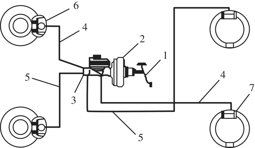
Figure 3.4 Diagonal dual-circuit brake system. (1) brake pedal; (2) vacuum booster; (3) tandem master cylinder; (4, 5) brake pipe lines; (6) disc brakes; (7) drum brakes.

Figure 3.5 Longitudinal motion of a vehicle and rotary motion model of a wheel. (a) Longitudinal motion of a vehicle; (b) Rotary motion.
3.3.3.2 Anti-lock Braking System Controller Design
- Principle of logic threshold control[5]
Take the wheel angular acceleration (or deceleration) as the main control threshold value and the wheel slip ratio as an auxiliary control threshold value. Using any of them alone has some limitations. For example, if the wheel angular acceleration (or deceleration) is taken as the control threshold alone, when the car strongly brakes at high speeds on a wet road, the wheel’s deceleration may reach the control threshold, even if the wheel slip ratio is far away from the unstable region. In addition to the driving wheels, if the clutch is not disengaged during braking, the large inertia of the wheel system will cause the wheel slip ratio to reach the unstable region while the wheel’s angular deceleration seldom reaches the control threshold value, which will affect the control effect seriously. If the wheel slip ratio is taken as the control threshold alone, it is difficult to ensure the best control effect in a variety of road conditions because the slip ratios corresponding to the peak adhesion coefficients vary widely (from 8% to 30%) in different road conditions. Thus, taking the wheel’s angular acceleration (or deceleration) and the wheel slip ratio as the control thresholds together will help the road identification and improve the adaptive capacity of the system. Anti-lock logic enables the wheel slip ratio to fluctuate around the peak adhesion coefficient, to obtain larger wheel longitudinal and lateral forces, and guarantees a shorter braking distance with good stability. The whole control process is shown in Figure 3.6.
In the initial stage of braking, the brake pressure rises as the driver depresses the brake pedal, and the wheel’s angular deceleration gradually increases until it reaches a set threshold value
 This is the first stage of the whole loop. In order to avoid the pressure being decreased while the slip ratio is still within the range corresponding to the wheel’s stable region, the reference slip ratio should be compared with the threshold value Sopt (see Figure 3.2). If the reference wheel slip ratio is less than Sopt, the wheel slip ratio is still small, and the control process goes to the second stage (the pressure holding stage). The inertia effect on the vehicle makes the wheel slip ratio greater than Sopt, which indicates that the wheel has entered the unstable region. Thus comes the third stage of the control process (the pressure decrease stage). As the wheel pressure decreases, the wheel begins to accelerate due to the vehicle inertia until the deceleration is smaller than
  (absolute values are compared). Then the fourth stage (the pressure holding stage) starts. Hereafter, because of inertia, the wheel is still accelerating until the acceleration reaches the threshold value + A. The pressure increases until the acceleration drops to + A, and the wheel is in the stable region again. The fifth stage begins. In order to keep the wheel in the stable region for longer, the shifting between the pressure increase and hold should be quick, and a low increasing rate of the pressure is maintained. This is the sixth stage. This stage lasts until the wheel’s angular deceleration reaches the threshold value again. Then, the pressure decrease stage begins and the next pressure regulation loop starts.
 - Logic threshold control flow
According to the logic threshold control theory described above, the control flow diagram is shown in Figure 3.7.
- Simulation and analysis
In order to verify the effect of the anti-lock braking system and improve the control algorithm, simulation or experimentation should be carried out. As an example, a simulation was done to a vehicle (parameters are shown in the appendix) in a MATLAB/Simulink environment to compare the braking performance with an uncontrolled braking system and with a logic threshold control anti-lock braking system. Assuming that the car moves on a road with a high adhesion coefficient with the initial speed of 20 m/s, and an expected slip ratio value of 0.16. The ODE45 algorithm was used and an automatic step size was chosen. The simulation results are shown in Figures 3.8–3.13.
Figure 3.8 shows the comparison of the longitudinal acceleration in two cases. When the car is equipped with a logic threshold control anti-lock braking system, it can take full advantage of the road’s adhesion coefficient, and have larger longitudinal acceleration and a much shorter braking distance (see Figure 3.9).
Figure 3.10 and Figure 3.11 show the comparison of the slip ratios of the front and rear wheels in two cases. The front and rear wheels of the car with an uncontrolled brake system are almost locked in about 1 second, and then they start slipping; the wheels of the car with the control system would not be locked during braking. The slip ratio slightly changes around the optimum value.
Figure 3.12 and Figure 3.13 show the comparison of the front and rear wheel speed. The results are same as those shown in Figure 3.10 and Figure 3.11.
Table 3.1 shows the comparison of the parts of the braking performance. The RMS value of the longitudinal acceleration increases from 6.6740 m/s2 to 7.5570 m/s2, and the front and rear wheel slip ratio’s RMS reduces from 0.8101 and 0.8054 to 0.2237 and 0.2574, which means that the performance is increased or decreased by 11.68%, 72.39% and 68.04% respectively. In addition, the braking distance was reduced from 27.418 m to 23.554 m.
As can be seen, the rational design of the wheel anti-lock braking system controller makes it possible to make full use of the road adhesion coefficient, shortening the braking distance and guaranteeing a good braking performance.

Figure 3.6 ABS control system’s process on a high adhesion surface.

Figure 3.7 The ABS logic threshold control flow.

Figure 3.8 Comparison of the longitudinal acceleration.

Figure 3.9 Comparison of the braking distance.

Figure 3.10 Comparison of the front wheels slip ratio.

Figure 3.11 Comparison of the rear wheel slip ratio.

Figure 3.12 Comparison of the front wheel speed.

Figure 3.13 Comparison of the rear wheel speed.
Table 3.1 Partial simulation results (rms).
| Performance | Logic threshold control | Uncontrolled |
| Longitudinal acceleration (m/s2) | 7.5570 | 6.6740 |
| Front wheel slip ratio | 0.2237 | 0.8101 |
| Rear wheel slip ratio | 0.2574 | 0.8054 |
3.4 Traction Control System
3.4.1 Introduction
When a vehicle accelerates on a low adhesion coefficient road or on a bisectional road, the driving wheels may slip resulting in a sideslip for rear-wheel driving cars and a difficulty in controlling the direction for front-wheel driving cars. The car's traction, handling stability, safety, and comfort will all influence this phenomenon.
The traction control system (TCS) is also known as the Acceleration Slip Regulation system (ASR). Its function is to: prevent the driving wheels from slipping excessively; keep the driving wheel slip ratio in the optimal range; guarantee direction stability; ensure the vehicle handling and dynamic performance; and to improve the vehicle driving safety.
When accelerating, the longitudinal adhesion coefficient increases along with the driving wheel slip ratio, where it reaches to a peak when the slip ratio increases to ST. It begins to decrease when the slip ratio increases further from this point, as shown in Figure 3.14. Here, the relationship between the lateral adhesion coefficient and the longitudinal slip ratio is also indicated. The lateral adhesion coefficient decreases rapidly when the longitudinal slip ratio increases. So, the car can get a greater longitudinal and lateral adhesion coefficient if the slip ratio is between 0 and ST. When the slip ratio is greater than ST, the longitudinal and lateral adhesion coefficient decreases rapidly, which will cause the loss of steering ability or even sideslip. Therefore, in order to guarantee good traction, handling, safety, and comfort in a starting or accelerating vehicle, the driving wheel slip ratio should be controlled by ST.

Figure 3.14 Slip ratio and adhesion coefficient curve.
3.4.2 Control Techniques of TCS[6]
Since the slip ratio of the wheel cannot be directly regulated, the most common technique is to adjust the torque on the wheel in order to control the motion of the wheel. The torque adjustment of the wheel can be realized by manipulating the engine output torque, transmission output torque, and braking torque on the wheel.
- Adjusting the engine output torque
For internal combustion engine cars, the torque transmitted to the driving wheels can be varied by adjusting the engine output torque, and then control of the driving wheel slip ratio can be achieved. There are three main ways to regulate the engine output torque. One is to control the angle of the throttle to change the engine output torque. This method has the advantage of being smooth and continuous, but it has to combine with other control methods to overcome the shortcoming of being slow to respond. The second is to adjust the ignition parameter. The engine output torque can be controlled by reducing the ignition timing or even temporarily stopping the ignition. This method has the advantage of having a rapid response, but it may cause an incomplete combustion and worsen the emissions. Another option is to alter the fuel supply. The engine output torque can be reduced by reducing or suspending the fuel supply; this is a relatively easy approach to implement but it may cause an abnormally working engine and influence its life and emissions.
- Differential lock control
A feature of the common symmetric differential is that it can differently distribute the rotational speeds but equally distribute the torques. So, when a car is driving on a bisectional road, the driving force on a high adhesion coefficient road can’t be fully used if the driving wheel slip ratio on the low adhesion coefficient road is too large. The traction performance of the car may be affected. The differential locking method can control the locking valve to lock the differential moderately according to the left and right driving wheel slip conditions and the road condition to keep the slip ratios of the driving wheels in a reasonable range. The driving forces of the wheels on a high adhesion coefficient road can be fully used, but the cost of this method is relatively high.
- Clutch or transmission control
When the driving wheel slip ratios are too large, the torque transmitted to the drive wheels can be reduced by controlling the engagement of the clutch, thus preventing excessive slip of the wheels. In addition, reducing the torque transmitted to the drive wheels can also be realized by reducing the transmission ratio. This control method should not be used alone because of the shortcomings of the slow response and the unsmooth changes of the torques.
- Braking torque adjustment
For a large slip ratio driving wheel, the slip ratio can be kept in the optimum range by controlling the braking torque. This is a commonly-chosen technique, which is normally used in conjunction with the engine torque adjustment method. The engine output torque must be regulated when the brake is applied to avoid excessive consumption of engine power. This control method has quite a good effect when the speed is not too high (less than 30 km/h), and the two driving wheels are on the bisectional road. However, it cannot be used for a long time and should not be used when the vehicle speed is high.
Figure 3.15 shows the simplified schematic of a TCS with integrated control methods of the engine throttle opening control and the wheel braking torque control. The system consists of sensors, hydraulic components, ECU, brake adjusters, and other components. When the car starts, the signals collected by the wheel speed sensors are sent to the ECU. After these signals are processed, the ECU gives commands to control the brake adjuster and the throttle angle according to the designed control strategy. The slip ratios are then regulated.

Figure 3.15 Structure of a TCS. 1. Front wheel speed sensor. 2. Front wheel brake. 3. Hydraulic components. 4. Brake pedal. 5. Rear wheel speed sensor. 6. Rear wheel brakes. 7. Sub-throttle actuator. 8. Throttle pedal. 9. Transmission. 10. ABS brake adjuster. 11. TCS brake adjuster. 12. Sub-throttle position sensor. 13. Main throttle position sensor. 14. Engine. 15. ECU. 16. Warning light. 17. Cut-off switch. 18. Working light.
3.4.3 TCS Control Strategy
Just as with the ABS, different methodologies have been used for the controlling of the TCS. At present, the main control strategies are: logic threshold control; PID control; optimal control; sliding mode variable structure control; fuzzy control; and neural network control[7].
- Logic threshold control
Logic threshold control is now the most widely-used method in vehicle control. The main idea is to first set a target slip ratio value, and then compare the driving wheel slip ratio with the reference one. If the driving wheel slip ratio exceeds the threshold or the target value, the control system sends the output regulating instructions to keep the driving wheel slip ratio or wheel acceleration close to the target value. When the driving wheel slips excessively once again, the control system begins to work until the slip ratio comes down to the target value. This is a conventional control method. It has the benefits of a simple structure, the small amount of computational effort that is needed, and it has a short time lag. However, it has the shortcomings of having fluctuations, poorer stability, and lacking adaptive capability.
- PID control
The PID control method can control the slip ratio by regulating the engine output torque or the braking torque. The system's input is the difference between the target slip ratio and the actual slip ratio. To keep the actual slip ratio close to the target slip ratio, this method feedbacks the throttle angle, which is calculated according to the input, to the engine to adjust the output torque of the engine, or it controls the braking system to change the braking torque. The conventional PID controller is simple and easy to implement. However, the control effect is not ideal in solving complex and nonlinear problems such as traction control, because of the difficulty in the mathematical modeling and the uncertainty of the vehicle parameters and environmental factors. Therefore, in order to get a better control effect, a conventional PID algorithm is usually used together with other control methods in the traction control problem. The block diagram of a PID controller is shown in Figure 3.16[8].
- Fuzzy logic control
It has been mentioned before that a car is a complex dynamic system and its working environment is complicated, so the traction control system is a complex nonlinear system. It is difficult to get the desired control results if conventional control methods are used. Fuzzy logic control does not require the precise mathematical model of the system. It is robust enough to accept changes in the system parameters and it allows time-varying, nonlinear, and complex systems. Therefore, it is suitable for the traction control system. In addition, fuzzy logic control theory has a better effect in solving the control problem of complex systems if used in conjunction with other control methods. The fuzzy PID control method has been currently applied in traction control systems. When using the PID method, the parameters Kp, Ki, and Kd need to be adjusted online constantly, and the adjustment of these parameters is a difficult task. However, after a reasonable fuzzy control rule table is designed, the fuzzy controller is a feasible and practical method for adjusting the three parameters of a PID controller.
- Sliding mode variable structure control
The characteristics of sliding mode variable structure control determine that the change of parameters and the external environment disturbance will not affect the control results when the controlled system is in the sliding mode motion. This method is therefore very robust, and it is suitable for use on the traction control system.
To design a sliding mode controller, the driving wheel slip ratio should be taken as the control target, and the target ratio S0 as the input threshold; the braking torque, the engine output torque, or the throttle angle should be taken as the control parameters. The controller regulates the control parameters to adjust the driving torque and thus leads to the change of the drive wheel rotational speed. The actual slip ratio can be kept close to the target slip ratio.
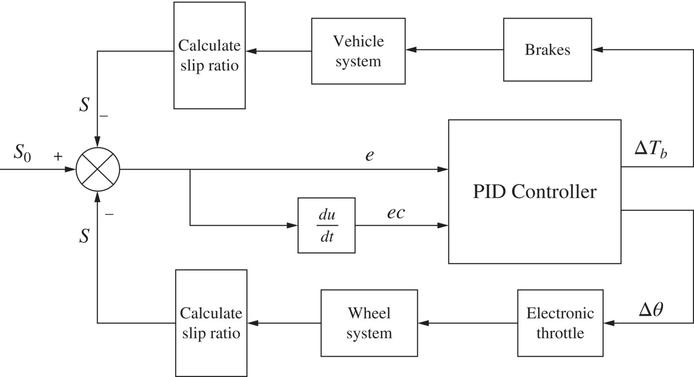
Figure 3.16 Block diagram of the PID controller of TCS. S0 Target slip ratio; S Actual slip rate; e Error; ec Error rate of change; Δθ Throttle opening degree increments; ΔTb Braking torque increment.
3.4.4 Traction Control System Modeling and Simulation
- Dynamic model
The dynamic model of a traction control system includes the sub-models such as the engine model, driveline model, tyre model, brake system model, and vehicle model. The tyre model, brake system model, and vehicle model can be established in the same way as in the ABS control system.
The engine model expresses the relationship between the output torque and the rotation speed. The modeling approach is to use a high-order polynomial to fit the mathematical relationship between the output torque and the speed on the basis of the experimental values, or the engine load characteristic curves corresponding to different throttle angles. A third order polynomial is commonly used, as follows:
(3.18)
where Te is the engine torque (Nm), a0, a1, a2, a3 are the fitting coefficients, and ne is the engine speed (r/min).
The throttle angle changes rapidly when the car is starting or changing speed, so it takes time for the engine to reach steady-state from a transient state. Therefore, the engine lags in response to the step inputs of the throttle angles. To describe the dynamics of its output characteristics, the engine is generally treated as a first order model with pure delay[8], and the transfer function can be expressed as:
(3.19)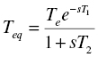
where Te is the steady-state torque, Teq is the dynamic torque, T1 is the system lag time constant, T2 is the system time constant, and s is the Laplace variable.
- Simulation and analysis
The literature[8] analyzes a bus TCS system with different control strategies. Figure 3.17 shows the slip ratio simulation results from the application of fuzzy PID control, and Figure 3.18 shows the wheel speed and the vehicle speed curve varying with time. As can be seen, the slip ratio stays stable near the desired value rapidly for the bus with TCS, which gives it better acceleration.

Figure 3.17 Slip ratio curve.

Figure 3.18 Vehicle speed and wheel speed curves.
3.5 Vehicle Stability Control
With the extensive application of ABS and TCS in the 1980s, it was noticed that proper modification of their control algorithms could give the systems the ability to actively maintain the vehicle body stability. Then the idea of vehicle stability control (Vehicle Stability Control, VSC, also known as the electronic stability program, ESP) was put forward. By adding active yaw control, longitudinal and lateral dynamics control could be achieved over the vehicle and accidents avoided when steering. In 1992, based on the ABS and TCS system, McLellan et al.[9] proposed the idea of the motion control of a vehicle in GM. The differences between the car’s motion parameters and the control targets were used as the feedbacks to control the wheel slip ratio, and thus the motion of the car could be controlled[9].
In the mid-1990s, Bosch launched the first VSC product, which marked the technology of the yaw stability control and its advances towards maturity[10]. Based on the ABS and TCS systems, the Bosch VSC system required the installation of a steering wheel angle sensor, brake master cylinder pressure sensor and throttle angle sensor in order to obtain the driver's intention, and then the expected tracking curve could be calculated using a pre-established driver model. The information of the yaw rate, lateral, and longitudinal acceleration could be obtained through the gyro in the VSC system. Based on all this information, if the VSC system judged that the car's current trajectory deviated from the driver's expectations, it initiated the direct yaw control (DYC) to maintain the vehicle stability and to avoid accidents.
Toyota and BMW also introduced their own VSC products. The lateral acceleration sensors and yaw rate sensors were used to measure the vehicle position directly in their systems, and application of the stability control system has been extended greatly.
After the statistical analysis of a large number of traffic accident data, the National Highway Traffic Safety Administration of the United States reached the conclusion that vehicle stability control systems are the most effective active safety control technology for vehicles at present. The collision accident ratio of passenger cars installed with VSC systems have declined by 34%, and rollover accidents dropped 71%[11].
3.5.1 Basic Principle of VSC
One of the basic principles of any VSC system is to identify the driver’s intention and represent the expected motion of the car by sensors and arithmetic logic. The actual motion of the car is then measured and estimated. If the difference between the actual and the desired motion is greater than a given threshold value, the VSC begins to regulate the longitudinal forces on the wheels according to the set control logic. The yaw acting on the car is changed, which may lead to the car’s actual motion becoming closer to the expected motion. A cornering car is used as the example to explain the VSC control principle, shown in Figure 3.19. When the vehicle has a tendency to oversteer, the VSC imposes the brakes on the external front wheel; this generates a yaw moment in the opposite direction to the vehicle as it corners which will take the car back to the desired path.
When the car tends to understeer there are two ways in which the VSC can interfere with its motion. One is to apply the brakes on the inner rear wheel to generate a yaw moment in the same direction as the vehicle cornering to increase the vehicle yaw motion. The other is to reduce the engine output torque to change the lateral forces of the front and rear axles, which will produce a yaw moment in the same direction as the vehicle cornering.

Figure 3.19 VSC system control principle.
3.5.2 Structure of a VSC System
As shown in Figure 3.20, the VSC is generally comprised of three parts: sensors, an electronic control unit (ECU) and a hydraulic control unit (HCU)[12]. The sensors are steering angle sensors, wheel speed sensors, gyroscopes, throttle opening sensors and master cylinder and wheel cylinder pressure sensors. The ECU generally uses embedded systems such as ARM or DSP, and also includes the sensor signal conditioning circuit, the solenoid valve control circuit, the pump motor control circuit, CAN bus communication circuit, detection and protection circuit, and other parts. The HCU is mainly composed of solenoid valves, a pump motor, and a special hydraulic circuit module. Figure 3.21 shows the internal VSC structure when the controller and the actuator are separated.

Figure 3.20 VSC system components.

Figure 3.21 Internal structure of a VSC system.
The sensors used on a VSC system are of two types. One type is used to perceive the driver’s actions, such as the steering wheel angle sensor, master cylinder pressure sensor, and throttle angle sensor, which can measure the action and the extent of steering, braking, and accelerating that the driver applies to the car. The throttle angle sensor and steering angle sensor are shown in Figure 3.22. The other type is used to gather information about the vehicle running state, such as the wheel speed sensors, the wheel cylinder pressure sensors, and the gyroscope. The gyroscope shown in Figure 3.23 can measure the tri-axial angular velocities and accelerations.

Figure 3.22 Throttle angle sensor and steering angle sensor. (a) The throttle angle sensor, (b) The steering wheel angle sensor.

Figure 3.23 Vehicle gyroscope.
An ECU generally has two microprocessors, one for dealing with the control logic, and the other for fault diagnosis and treatment. The two microprocessors exchange information with each other via an internal bus. In addition to the microprocessors, the ECU also includes a power management module, the sensor signals input module, a hydraulic regulator driving module, a variety of indicators interface, and a CAN bus communication interface. Most ECUs are mounted together with the hydraulic regulator through the electromagnetic coupling between the solenoid coils and the spool of the solenoid valve.
According to the information obtained from the steering wheel angle sensor and the master cylinder pressure sensor, the ECU determines the driving intention and calculates the ideal motion state (such as the desired yaw rate, etc.). After comparing the measured actual motion with the ideal car motion, the amount of yaw moment that should be applied to keep the car stable can be determined by the control logic. Finally, the ECU adjusts the brake cylinders of the braking system through the hydraulic regulator to generate the needed yaw moment. If necessary, the ECU communicates with the engine management system (EMS) to change the driving force of the driving wheels to change the car’s motion. The sensors measure the updated car motion parameters and send the information to the ECU to conduct the next control cycle in order to continue to keep the car stable.
Figure 3.24 shows the working principle of the VSC–hydraulic actuator unit. The VSC control logic requires that each wheel can be braked at any necessary time, so the hydraulic brake pipeline in the car equipped with VSC must guarantee that the brakes can be applied to every single wheel without affecting other wheels. Normally, the hydraulic pipeline of the VSC is constructed by adding four solenoid valves on that of the ABS. Two normally open valves between the main pipeline and the master cylinder will be energized to close the main oil pipeline immediately the HCU starts working, and then the driver's braking operation will not function. A further two valves, which are normally closed, are located in two additional pipelines connecting the master cylinder and the oil return pump, and these lines are normally closed. Only when the driver steps on the brake pedal will the brake fluid flow into the wheel cylinders. If the driver applies the brakes when the VSC works, the normally closed valve will be electrified to an opened state to keep the brake fluid flowing into the low pressure accumulator.
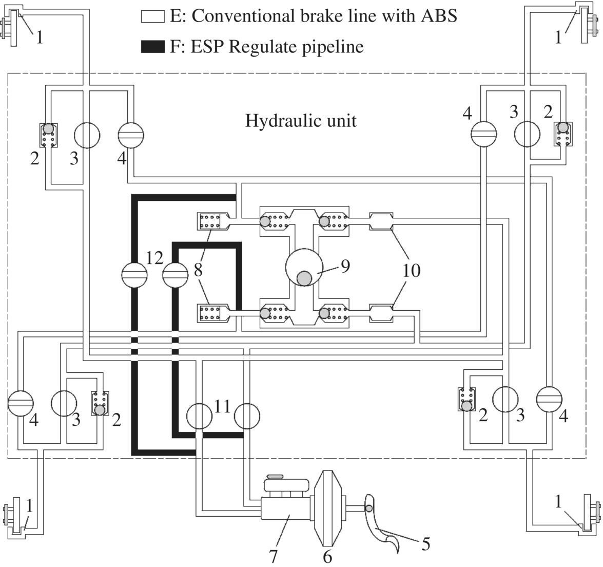
Figure 3.24 The hydraulic brake pipeline layout in a vehicle with VSC. 1 Brake caliper. 2 Brake valve. 3 Entry for solenoid valve. 4 Exhaust gas solenoid valve. 5 Brake pedal. 6 Brake booster. 7 Brake master cylinder. 8 Accumulator. 9 Jet pump. 10 Buffer. 11 Transform solenoid valve. 12 Master solenoid valve.
The active increase of pressure of the VSC is carried out by the oil return pump. When the brakes need to be applied on one wheel, the two normally open solenoid valves on the main pipeline will be closed, and the normally open valves on the pipeline with the other wheel cylinders will be closed too; the oil from the return pump can only flow to the wheel cylinder which needs higher pressure. Thus, the pressure in one single wheel cylinder should be increased.
3.5.3 Control Methods to Improve Vehicle Stability
When a vehicle is moving with the lateral acceleration of less than 0.4g (linear region), the driver can effectively control the vehicle without entering the unstable region. When the motion of the car is in the unstable region, the vehicle stability control system helps to decrease the sideslip angle rapidly, and to return the car back into the stable region quickly[13].
There are many ways to improve vehicle stability, amongst which active steering control, front and rear axle roll stiffness distribution control, and direct yaw moment control are those most commonly used.
- Active steering control
There are many possible methods of applying active steering control, such as 4-wheel steering (4WS), Steer by Wire (SBW), and active front wheel steering (AFS). By introducing motion parameters such as yaw rate or lateral acceleration as the feedback, the active steering control method can improve the handling and stability of the car in the linear region and, to some extent, prevent the sideslip angle from appearing. However, adjusting the car's attitude by the steering would be very difficult if the lateral forces of the tyres tend to reach saturation. Therefore, the effect of this method is not obvious when steering in the nonlinear region and with very large sideslip angles.
- Cornering stiffness distribution control
Vehicle stability has a considerable relationship with the cornering stiffness of the front and rear tyres, and this relationship determines the car's steering characteristics. The vehicle stability factor can be expressed as:
where kf is the front tyre cornering stiffness, kr is the rear tyre cornering stiffness, and m is the vehicle mass.
Equation (3.20) shows that the sign of K is determined by
 , which is closely related to the cornering stiffness of the front and rear tyres. Practically, the tyre cornering stiffness changes with the working load. By introducing the motion state parameters as the feedback to a vehicle with an active suspension system, the system can adjust the axle load distribution which will change the cornering stiffness of the front and rear tyres. However, this control method has serious limitations. First, the vehicle must have an active suspension system. Second, this method is only effective when the lateral acceleration is large. And finally, the vehicle longitudinal acceleration generated by the longitudinal force has a great impact on the axle load transfer.
 - Direct yaw moment control
Direct yaw moment control, also known as differential braking control, is an active control method which changes the vehicle state by applying different braking forces on different wheels. This is a very effective way of changing the yaw moment and adjusting the motion attitude of the car. This method functions when the car is braking, driving, steering, and even in a combination of conditions; it also works effectively when the sideslip angle is large. So differential braking is the most suitable method for vehicle stability control, especially when the tyre’s adhesion reaches the limit[14].

3.5.4 Selection of the Control Variables
The VSC system needs to solve two main problems, track keeping and vehicle stability, which can be described by the sideslip angle and the yaw rate respectively. The sideslip angle and yaw rate reflect the essential characteristics of the vehicle steering, and the relationship between them determines the stable state of the car and characterizes the stability from different sides. The sideslip angle represents the lateral velocity and track deviation of the car when steering, which emphasizes the description of the track keeping problem. The yaw rate is the reflex of the changing speed of the heading angle when steering, which determines the steering characteristics of the car: understeering or oversteering. The sideslip angle can be used to describe stability.
- Relationship between yaw rate and vehicle stability
The two degrees of freedom linear vehicle model shows that the motion of a car is mainly described by the longitudinal velocity, lateral velocity, and yaw rate. Longitudinal velocity and lateral velocity determine the vehicle sideslip angle, and the integral of the yaw rate is the yaw angle. Take θ as the car heading angle, it is equal to the sum of the sideslip angle and yaw angle[1].
(3.21)
where ψ is the vehicle yaw angle.
When the sideslip angle is small, the car's heading angle is determined by the yaw angle or yaw rate mainly. The larger the heading angle, the smaller the turning radius will be, and vice versa. Understeering or oversteering, which are the two key steering characteristics of a car, can be estimated from the turning radius. Therefore, when the sideslip angle is small, the yaw rate can represent the car’s state of stability. Also, because the yaw rate signal can be directly obtained from the sensors on the car, the yaw rate is an important control variable in most vehicle stability control strategies.
- The relationship between sideslip angle and vehicle stability
The analysis above is based on the assumption that the sideslip angle is small, but the sideslip angle is generally large when severe sideslip occurs. In this case, the vehicle stability cannot be accurately described by using the yaw rate, but the sideslip angle can be used instead. Therefore, the sideslip angle is normally limited to relatively small values in vehicle stability control systems.
Some scholars have analyzed the relationship between the sideslip angle and vehicle stability. The β method is the most representative idea that has been put forward[15]. The influence of the sideslip angle on vehicle stability according to this method, is presented here.
The β method explains the relationship between the sideslip angle and stability by analyzing the impact of the sideslip angle on the yaw moment and the lateral force. The relationship of the yaw moment with the lateral force and the slip angle can be obtained from the vehicle dynamics model. Taking the front tyres as the example, the lateral force curves when they move on the road with the friction coefficient of 0.8 and 0.2 are shown in Figure 3.25.
As can be seen from Figure 3.25, on a low adhesion road the lateral force gets saturated even when the sideslip angle is small, and the lateral force provided is much smaller than that on the high adhesion road. The simulation results of the impact of the sideslip angle on the yaw moment and the lateral force are shown in Figures 3.26 and 3.27.
The β method shows that the vehicle tends to be stable when the yaw moment is positive or increases with the vehicle sideslip angle; otherwise, the car may lose stability. It can be seen from Figure 3.26 that a positive angle produces a positive yaw moment and lateral force, and a negative angle produces a negative yaw moment and lateral force when the sideslip angle is zero. However, the increment of the yaw moment and the lateral force decreases with the increase of the front wheel turning angle, which indicates that the tyre forces tend to enter the saturated zone as the sideslip angle becomes larger. The vehicle yaw moment increases at first and then decreases along with the increase of the sideslip angle, and it gets close to zero when the sideslip angle is relatively large. The lateral force decreases with the increase of the sideslip angle and reaches a peak value when the sideslip angle is considerably large, which means that even if the driver turns the steering wheel, the yaw moment cannot be produced. That is why the vehicle is difficult to manipulate under large sideslip angle conditions.
Figure 3.27 shows the relationship of the yaw moment and the lateral force when the adhesion coefficient is low. It can be seen that as the adhesion coefficient between the tyre and the road’s surface decreases, the yaw moment reaches zero more rapidly with the increase of the sideslip angle, and the lateral force gets saturated more quickly too. Therefore, the lower the adhesion coefficient, the more difficult it is for the driver to attain the yaw moment by turning the steering wheel. The lower the adhesion coefficient, the greater the impact of the sideslip angle on the vehicle stability, and the maximum sideslip angle needed to keep the vehicle stable is smaller. Therefore, when the vehicle moves on a low adhesion road, the sideslip angle should be strictly limited in order to maintain stability.
The conclusion is that dangerous situations cannot be avoided completely by only controlling the yaw rate, especially when the vehicle is running on a low adhesion road. Thus, in addition to considering the rolling of the vehicle body, the degree of deviation from the current track should also be considered so, the sideslip angle must be controlled. As the sideslip angle cannot be measured directly by the sensors on the vehicle, the estimation method has to be used, although the accuracy may be affected to some extent. In practical VSC systems, the range of the sideslip angle is generally set to avoid an unexpected intervention caused by inaccurate estimations.

Figure 3.25 Front wheel lateral force curve.

Figure 3.26 The impact of the sideslip angle with an adhesion coefficient of 0.8, at 20 m/s.

Figure 3.27 The impact of the sideslip angle with an adhesion coefficient of 0.2, at 20 m/s.
3.5.5 Control System Structure
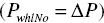
In order to meet the needs of vehicle stability control, VSC systems generally adopt a hierarchical control structure[1,14], which is shown in Figure 3.28. The control system gets the inputs from the sensors installed on the vehicle, and the motion parameter estimator. This is due to the motion parameters (such as the longitudinal vehicle speed, the sideslip angle, and the road adhesion coefficient) which are difficult to measure by sensors directly; therefore, those parameters need to be estimated based on the measured signal. Taking the deviation between the desired motion and the actual motion as the input, the upper motion controller is responsible for calculating the nominal yaw moment MYawNo needed to eliminate the motion deviation. The lower actuator controller distributes the braking force on each wheel according to the nominal yaw moment and calculates the nominal braking pressure PWhlNo of each wheel. Thus, the brake pressure is controlled by the lower controller. The required forces can then be applied to the vehicle through the interaction between the tyre and the road. There are inner and outer feedback control loops in the hierarchical control system. The outer feedback control loop provides the nominal yaw moment for the inner feedback loop, and the inner feedback control loop adjusts the tyre forces by the nominal braking pressure.

Figure 3.28 The hierarchical control system in VSC systems.
3.5.6 The Dynamics Models
Theoretical research on VSC usually needs the establishment of models such as the nonlinear vehicle model, the linear half vehicle model, and the hydraulic system model. The nonlinear vehicle model is the controlled objective, and it must contain a nonlinear tyre model to study the impact of the lateral force on the body motion. The linear half vehicle model provides the desired values of the motion parameters for reference. Since VSC controls the body motion through the hydraulic brake system, the complete hydraulic brake system model and the wheel braking model are essential.
- The desired value calculation model
The two degrees of freedom linear model is widely used as the desired value calculation model in VSC systems because it is simple and contains most of the important parameters describing the lateral motion like the body mass, front and rear tyres cornering stiffness, and wheelbase (Figure 3.29).
The dynamics equations are
(3.22) (3.23)
where δf is the front wheel turning angle, Iz is the inertia moment of the vehicle about the z-axis, lf, lr are the distances between the C.G. and the front and rear axle, vx, vy are the longitudinal and lateral velocities of the C.G., r is the yaw rate, and kf, kr are the front and rear tyres’ cornering stiffness.
The desired yaw rate βd and the sideslip angle rd can be calculated by (3.24) and (3.25)[16]:
- The actual motion model
There are many methods of establishing the dynamics model of a vehicle, amongst which modeling by formulating the equations and by using software are commonly used. As an example, a seven degree of freedom car model built by formulating the equations is presented. A car can be simplified as a seven degree of freedom model which includes longitudinal, lateral, and yaw motion of the body and rotational movements of the four wheels, as shown in Figure 3.30.
The dynamics equations of the body are:
(3.26) (3.27)
 (3.28)
where


and where vx is the longitudinal velocity, vy is the lateral velocity, r is the yaw rate, δfi s the front angle, Fxi, Fyi
 are the longitudinal forces and lateral forces of the wheels, m is the car mass, Iz is the inertia moment of the car about the z-axis, lf, lr are the distance between the C.G. and front and rear axles, and Df, Dr are the front and rear tracks.


Figure 3.29 Two degrees of freedom linear vehicle model.

Figure 3.30 The seven degrees of freedom nonlinear dynamic model.
3.5.7 Setting of the Target Values for the Control Variables
- The ideal yaw rate
The ideal yaw rate is proportional to the steering wheel angle under certain vehicle speeds when the sideslip angle at the center of mass is small. The yaw rate gain relative to the steering wheel angle should be reduced appropriately when the vehicle speed increases to avoid the steering wheel being too sensitive at high speeds. Figure 3.31 shows the relationship between the ideal yaw rate and vehicle speed[17]. Each solid curve is with the same front wheel angle, and each dotted curve is the adhesion limitation of equal road adhesion coefficient. The ideal yaw rate is limited by the maximum force the road can provide.
It is reasonable to use the two degrees of freedom linear model to calculate the expected motion parameters, but the influence of the road adhesion coefficient on them is not embodied in the model. In different road conditions, the lateral forces must satisfy the following constraint:
(3.29)
When the sideslip angle is very small, thus:
(3.30)
So, the ideal yaw rate should also meet the following condition:
(3.31)
- The stability region of the sideslip angle
It can be seen that the sideslip angle threshold is closely tied to the adhesion coefficient through the above analysis by the β method. Because it is quite difficult to control the sideslip angle precisely, constructing a stable region of sideslip angle by using the sideslip angle and the yaw rate is a common practice. The boundary of the region can be described by the following equation:
where E1 and E2 are the constants of the stable boundary.
Equation (3.32) can be used as a control criterion of the sideslip angle, and it is also the basis for the yaw moment control algorithm design. The vehicle state can be considered to be stable when the inequality holds, while the vehicle will tend to oversteer when the inequality does not hold, which shows the necessity for the stability intervention.

Figure 3.31 The relationship between the ideal yaw rate and vehicle speed.
3.5.8 Calculation of the Nominal Yaw Moment and Control
The upper and lower controllers are the core parts in the layered control system of a VSC (see Figure 3.28).
- Design of the upper controller
When a vehicle is moving with an ideal yaw rate and the sideslip angle is within the stable range, the vehicle can be regarded as being in an ideal state. When the vehicle begins to lose stability, its motion state will be very different from the ideal one. At this time, the additional yaw moment ΔM is applied on the vehicle to stabilize the vehicle and make the actual vehicle state closer to the ideal. The upper controller calculates the value of the additional yaw moment ΔM, which consists of ΔMr, produced by the yaw rate controller, and ΔMβ, produced by the sideslip controller, as shown in Figure 3.32.
Some control algorithms can be used in the yaw rate controller, such as PID control, feed forward and feedback combined control, optimal control, sliding-mode control, and fuzzy logic control. Because the sideslip angle of the vehicle is difficult to control, the simple but practical PD controller is normally used to stabilize the vehicle when it tends to be unstable.
(3.33)
Then additional yaw moment can be obtained by the following equation:
(3.34)
- Design of the lower controller
The function of the lower controller is to convert the additional yaw moment to the actual values of the variables, such as wheel cylinder pressure or the braking torque, so the controller can apply the brakes on a single or multiple wheels.
When braking on different wheels, the effectiveness of the additional yaw moments generated by either decreasing the lateral forces or by applying the brakes is different. The yaw moments produced by braking the front wheels is very different from the moments produced by braking the rear wheels. When steering, the directions of the additional yaw moments caused by the braking force of the outer front wheel and by the lateral force are the same, which is opposite to the turning direction. So this is the most effective way to correct oversteering, while braking the inner rear wheel is most suitable to correct understeering (Figure 3.33).
Since the key task of the VSC system is to help the driver to fulfill his turning purpose, the order made by the control strategy should not violate the driver’s steering intention. So, the yaw moment needed must be calculated at any time. The steering angle δf, the steering wheel velocity
 and the difference between the actual yaw rate and the ideal yaw rate
  are used to judge the vehicle motion state. The decision of which wheel should be braked can then be made. Table 3.2 shows the detail strategy for a single wheel braking method. The positive sign of parameters is pointed to the left.
There are two main methods that the lower controller can employ to implement the control, the slip ratio control and the direct braking torque control[18,19].
- Slip ratio control
To establish the slip ratio control, two steps should be followed. First, the relationship of the yaw moment and the slip ratio needs to be determined and the change of the slip ratio of the wheel which is to be braked calculated according to the additional yaw moment. Second, the change to the slip ratio controller must be inputted to implement the control of the wheel.
Take the single wheel braking method, for example. In the event of a vehicle losing stability, the VSC system needs to apply the brakes on the front left wheel to produce a yaw moment to make the vehicle stable. According to the tyre models, the longitudinal and lateral forces on this wheel can be expressed as:
(3.35) (3.36)
where μx(S), μy(S) are the functions of the longitudinal and lateral adhesion coefficient, and Fz is the vertical load on the wheel.
The yaw motion produced by the variation of the front left wheel slip ratio can be obtained by the following equation:
where ΔM is the additional yaw moment, S0 is the slip ratio of the front left wheel at the moment the controller starts, which can be calculated by the speed signal from the wheel velocity sensor.
Based on equation (3.37), the variation range of the slip ratio ΔS can be fixed according to the control values of the yaw moment, and the increment of the wheel cylinder pressure ΔP can then be calculated. For convenience, if a PD control algorithm is adopted, ΔP can be obtained by the following equation:
(3.38)
When the driver doesn’t step on the brake pedal, the target pressure PwhlNo is the increment of the wheel cylinder pressure ΔP
 . When the driver applies the brakes, suppose the pressure in wheel cylinder is P0, thus the target pressure PwhlNo is calculated by equation (3.39)
 - Braking torque control
Braking torque control is different from the slip ratio control. Instead of using the slip ratio controller, the additional yaw moment is converted to the control quantity of the wheel cylinder pressure directly. The principle of the cylinder pressure calculation is: (a) to change the calculated additional yaw moment ΔM to the variation of the longitudinal forces of one-side wheels; and (b), to determine the wheel cylinder pressure change by using the wheel motion model. Taking the one-side wheels braking model as an example, the additional yaw moment can be expressed by the longitudinal forces in Equation (3.40)[16]
Because the front and rear wheels on the same side are controlled uniformly, the longitudinal forces of the wheels on the same side are approximately equal. If Fd is the expectation of the longitudinal tyre force,
 then equation (3.40) can be rewritten as:(3.41)
The wheel motion model is presented below[20]:
In equation (3.42), ω is obtained from the wheel velocity sensor, and Tt = 0 when braking (during normal running conditions, it can be calculated if the engine torque is known). The longitudinal tyre force can be expressed as:
(3.43)
To the drum brake:
(3.44)
So, the increment of the longitudinal tyre force is:
(3.45)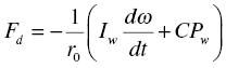
where
 Iw is the wheel’s inertia, Tb is the brake torque, Tt is the driving torque, r0 is the wheel radius, ω is the wheel’s angular velocity, Pw is the target pressure of the wheel cylinder, Aw is the brake shoe area, ub is the friction coefficient of the brake shoe, and Rb is the distance between the wheel center and the brake shoe.
 - Simulation and analysis
The simulation was done under the conditions that the car moved on two different roads with the adhesion coefficient of 0.9 and 0.4 at the speed of 120 km/h and 60 km/h respectively. The input steering wheel angle took the form of an amplitude increasing sine wave. The curve of the front wheel turning angle is shown in Figure 3.34. The simulation results are shown in Figures 3.35–3.40. Figure 3.35 to Figure 3.37 illustrate the yaw rate, sideslip angle, and the phase variation when the road adhesion coefficient is 0.9.
The simulation results are shown in Figures 3.38–3.40, when the road adhesion coefficient is 0.4.
From the simulation results, it can be concluded that the VSC can effectively keep the vehicle body stable. Without a VSC system, with the increase of the front wheel turning angle, the vehicle tends to be unstable. When the front wheel turning angle is big enough, the vehicle yaw rate and sideslip angle increase sharply. At this time, the vehicle will spin and deviate from the expected track significantly, and lose control completely. In the uncontrolled vehicle, as the vehicle speed is fixed during simulation, the yaw rate and sideslip angle have the tendency to increase indefinitely after the vehicle becomes unstable. But with the help of the VSC, the vehicle yaw rate and sideslip angle meet the expectations of the driver quite well. As can be seen from the phase plane diagrams shown in Figure 3.37 and Figure 3.40, the vehicle is in a stable state.


Figure 3.32 Logical diagram of the upper controller.

Figure 3.33 Yaw moment caused by braking on different wheels.
Table 3.2 The choice of the braked wheel.
|
|
δf | Vehicle state | Braked wheel | |
| + | + | + | oversteer | Front right |
| + | + | 0 | oversteer | Front right |
| + | + | − | oversteer | Front right |
| + | − | + | Without braking (no) | |
| + | + | 0 | understeer | Rear right |
| + | − | 0 | understeer | Rear right |
| + | 0 | + | oversteer | Front right |
| − | + | + | understeer | Rear left |
| − | + | 0 | understeer | Rear left |
| − | + | − | Without braking (no) | |
| − | − | + | oversteer | Front left |
| − | − | 0 | oversteer | Front left |
| − | − | − | oversteer | Front left |
| − | 0 | + | understeer | Rear left |
| − | 0 | − | oversteer | Front left |

Figure 3.34 Front wheel steering angle.

Figure 3.35 Yaw rate.


Figure 3.37 The phase diagram of the sideslip angle and sideslip angular velocity.

Figure 3.38 Yaw rate.


Figure 3.40 The phase diagram of the sideslip angle and sideslip angular velocity.
Appendix
| Vehicle parameters | Symbol | Unit | Value |
| Vehicle mass | m | kg | 1500 |
| Front/rear wheel to centroid distance | l f /lr | m | 1.219/1.252 |
| Inertia of pitching moment | I y |
|
2436.4 |
| Brake pedal force | F b | N | 220 |
| Brake master cylinder diameter | D m | m | 0.02222 |
| Transmission ratio of brake pedal mechanism | i b | - | 4.45 |
| Boosting ratio booster | B | - | 3.9 |
| Brake disc working radius | D f | m | 0.104 |
| Brake disc braking efficiency factor | C f | - | 0.8 |
| Front wheel cylinder piston diameter | D wf | m | 0.054 |
| Number of single clamp brake cylinders | n | 1 | |
| Brake master cylinder efficiency | η p | - | 0.75 |
| Brake drum working radius | D r | m | 0.100 |
| Brake drum braking efficiency factor | C r | - | 2.15 |
| Rear wheel cylinder piston diameter | D wr | m | 0.01746 |
| Sprung mass centroid height | h | m | 0.6 |
| Front/rear unsprung centroid height | h 1/h2 | m | 0.24/0.26 |
References
- [1] Rajamani R. Vehicle Dynamics and Control. Springer US, 2006.
- [2] Yu Z S. Automotive Theory, 4th edition. Mechanical Industry Press, Beijing, 2009.
- [3] Li C M. Automotive Chassis Electronic Control Technology. Mechanical Industry Press, Beijing, 2004.
- [4] Lu Z X. Automotive ABS, ASR and ESP Maintenance Illustrations. Electronic Industry Press, Beijing, 2006.
- [5] Chu C B. Study on automotive chassis systems hierarchical coordination control. PhD thesis, Hefei University of Technology, Hefei, 2008.
- [6] Wang D P, Guo K H, Gao Z H. Automotive drive anti-slip control technology. Automotive Technology, 1997, 4: 22–27.
- [7] Zhang C B, Wu G Q, Ding Y L, et al. Study on control methods of automotive drive anti-slip. Automotive Engineering, 2000, 22(5): 324–328.
- [8] Xiong X G. Study on control law of automotive drive anti-slip control system. Master's degree thesis, Hefei: Hefei University of Technology, 2010.
- [9] McLellan D R, Ryan J P, Browalski E S, Heinricy J W. Increasing the safe driving envelope - ABS, traction control and beyond. Proceedings of the Society of Automotive Engineers, 92C014, 1992: 103–125.
- [10] van Zanten A T, Erhardt R, Pfaff G. VDC, the Vehicle Dynamics Control System of Bosch. SAE Technical Paper, 950759.
- [11] NHSTA. Federal Motor Vehicle Safety Standards No.126: Electronic Stability Control Systems. http://www.nhtsa.dot.gov/, 2007.
- [12] van Zanten A T. Bosch VSC: 5 Years of Experience. SAE Technical Paper, 2000-01-1633.
- [13] Nishio A, Tozu K, Yamaguchi H, Asano K, et al. Development of Vehicle Stability Control System Based on Vehicle Sideslip Angle Estimation. SAE Technical Paper 2001-01-0137.
- [14] Wang D P, Guo K H. Study on the control principle and strategy of vehicle dynamics stability control. Journal of Mechanical Engineering, 2000, 36(3): 97–99.
- [15] Hac A. Evaluation of Two Concepts in Vehicle Stability Enhancement Systems. Proceedings of 31st ISATA, Program Track on Automotive Mechatronics and Design, Düsseldorf, Germany, 1998, 205–213.
- [16] Wang Q D, Zhang G H, Chen W W. Study on control of vehicle dynamics stability based on Sliding Mode Variable Structure. China Mechanical Engineering, 2009, 20(5): 622–625.
- [17] Liu X Y. Study on vehicle stability control based on direct yaw moment control. PhD thesis, Hefei University of Technology, Hefei, 2010.
- [18] Koibuchi K, Yamamoto M, Fukada Y, Inagaki S. Vehicle Stability Control System in Limit Cornering by Active Brake. SAE Technical Paper, 960487.
- [19] Tseng H E, Ashrafi B, Madau D, et al. The development of vehicle stability control at Ford. IEEE/ASME Transactions on Mechatronics, 1999, 4(3): 223–234.
- [20] You S H, Hahn J O, Cho Y M, Lee K I. Modeling and control of a hydraulic unit for direct yaw moment control in an automobile. Control Engineering Practice, 2006, 14(9): 1011–1022.