
4
Vertical Vehicle Dynamics and Control
4.1 Vertical Dynamics Models
4.1.1 Introduction
The complex environment of vehicles means that the frequency range of vibration of the components, which can affect the comfort of drivers and passengers, is quite wide. Usually, NVH features (i.e., noise, vibration, and harshness) are used to characterize comfort. Generally, the range of vibration frequency can be divided into: 0–15 Hz for rigid motion, 15–150 Hz for vibration and resonance, and above 150 Hz for noise and scream.
Normally, a typical range of the resonance frequency can be divided as follows:
- the vehicle body is in the range of 1–1.5Hz (the damping ratio ζ is approximate 0.3);
- the wheel jumping is in the range of 10–12Hz;
- for the drivers and passengers it is in the range of 4–6Hz;
- for the powertrain mount it is in the range of 10–20Hz;
- for the structure it is over 20Hz; and
- for the tyre it is in the range of 30–50Hz and 80–100Hz.
This chapter mainly introduces the vertical dynamics which involves optimizing the design of parameters for a suspension system. This means that designers should coordinate the contradictory performance indexes such that the optimal performance of a suspension system can be achieved. To achieve this, one should ensure that the dynamic models reflect the actual working environment of vehicles, which largely depends on the complexity, the objects, and the demanded precision.
Since vehicles are complex vibrating systems with multiple degrees of freedom, theoretically these systems will approach reality as the degrees of freedom increase. Therefore, it is natural to model the vehicles as various 3-dimensional models with dozens of degrees of freedom. From the point of view of comfort, the human–seat system is included in the systems when considering the responses to body vibration. For the road model, the systems include the input signals from the four wheels which are caused by road irregularities. These signals are different but they relate to each other. In addition, for vehicles which have low body stiffness and a long wheelbase, the bending and twist of the vehicle frame and body needs to be considered. If the effects from a powertrain mounting system need to be analyzed, one can separate this part from the vehicle body and consider the degrees of freedom relative to the vehicle body in the vertical direction. These methods will make the dynamic model closer to reality.
The increase of degrees of freedom indicates that more parameters are needed in the calculations. However, for some parameters, such as the mass, moment of inertia, and stiffness, etc., it is difficult to obtain precise values. Besides, the efficiency of the calculations is slowed down as the calculation precision increases. Thus, one should simplify the dynamic models of the vehicles by systematically considering the relative factors, such that the models are simple and can reflect reality.
4.1.2 Half-vehicle model
Assuming that the surface of the road is flat, which means the difference of the road’s surface by the two sides of vehicles can be ignored, one can establish a half-vehicle model with four degrees of freedom, as shown in Figure 4.1. For a half-vehicle model, following the dynamics equivalence, the vehicle body with mass m2 and moment of inertia I can be decomposed into m2f, m2r and m2c, which are, respectively, the mass of the front wheel, rear wheel, and center of mass. They satisfy the following conditions:
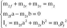
where ρy is the radius of gyration around the horizontal axis y. Thus one has:

Here,  is the distribution coefficient of the sprung mass. One has
 ![]() , when
, when ![]() . Statistically, the value of ε for most vehicles ranges from 0.8 to 1.2, which can be viewed as close to 1. for
. Statistically, the value of ε for most vehicles ranges from 0.8 to 1.2, which can be viewed as close to 1. for ![]() , the motions for m2f , m2r in the vertical direction are mutually independent. In this case, the vertical displacements x2f and x2r respectively on the front and rear wheel do not couple, and the main frequency is the same frequency as for the front and rear parts.
, the motions for m2f , m2r in the vertical direction are mutually independent. In this case, the vertical displacements x2f and x2r respectively on the front and rear wheel do not couple, and the main frequency is the same frequency as for the front and rear parts.

Figure 4.1 4-DOF half-vehicle model.
In Figure 4.1, a, b are the distances from the center of mass to the front/rear axle; ms is the vehicle mass; m1f, m1r are the front/rear wheel mass; Ic is the moment of inertia of the body around the transverse axle; ksf and cf are the front suspension stiffness/damping coefficient; ksr and cr are the rear suspension stiffness/damping coefficient; ktf and ktr are the front/rear tyre stiffness coefficient; x0f and x0r are road roughness of the front/rear tyre contact; x2 is the vertical displacement of the center of mass of the body; θ is the pitch angle; x2f and x2r are the vertical displacements of the front/rear end; x1f and x1r are vertical displacements of front/rear tyre; and c is the center of mass.
The motion equations of a 4-DOF half-vehicle model shown in Figure. 4.1 can be written as:
When the pitch angle θ is small, the following approximations can be reached:
The matrix form of the equations of motion of the 4-DOF half-car model is:
where [M] = diag[m2, Ic, m1f, m1r] is the mass matrix. The damping matrix is:

The suspension stiffness matrix is:

The tyre stiffness matrix is:

The road’s surface input matrix is:
The system output matrix is:
It is necessary to use the full-vehicle model with seven degrees of freedom for studying the roll input from the road. The modeling process is similar to the half-vehicle model, except that the equations need to consider the factors for describing the roll motion of the body and the vertical motion of the other two tyres, which will be illustrated later.
4.2 Input Models of the Road’s Surface
The roughness of the road’s surface is the main disturbance into a vehicle system. In order to predict how the vehicle will respond to the input from the road’s surface, it is necessary to describe the features of the road’s surface correctly. The measurement of a road’s surface roughness and the data processing, which needs specialized equipment, is important but time-consuming and not economical. This is the reason why this method has limited applications in engineering. Therefore, if a realistic road surface input model is established, it will prove a good foundation to the study of dynamic response and control.
4.2.1 Frequency-domain Models
From the study of the measurement data of a road’s surface roughness, it shows that when the vehicle speed is constant, the road’s roughness follows a Gaussian probability distribution, which is a stationary and ergodic stochastic process with a mean of zero. The power spectrum density (PSD) function and the variance of the road’s surface can be used to describe its statistical properties. Since the velocity power spectral density is constant, which satisfies the definition and statistical properties of the white noise, it can be used to fit the time domain models of the road’s surface roughness after the appropriate transformation. In the 1950s, people began to study the power spectrum of the road’s surface, and used it to evaluate the quality of the road’s surface and vehicle vibration responses. Until now, different methods for expressing the power spectrum of the road’s surface have been proposed. In 1984, the international standards organization (ISO) proposed the draft to describe the road’s surface roughness in the file ISO/TC108/SC2N67. According to this, China also drew up the measurement data report of the road’s surface spectrum of the mechanical vibration (GB7031-2005). Both of the two reports suggested the fitting formula for the road’s surface power spectrum Gq(n) is[1]:

where n is the spatial frequency (m–1), which is the inverse of the wavelength λ and means the numbers of waves per meter; n0 = 0.1 is the referred frequency (m−1); Gq (n0) is the coefficient of the road’s surface irregularity (m3), which is the value of the road’s surface PSD under the referred frequency n0; and p is the frequency exponent, which is the slope of the line of the log-log coordinates, and decides the frequency structure of the road’s surface PSD.
In addition, the root-mean-square values of various road surfaces to describe its intensity, or the mean power of the road’s surface stochastic exciting signals are defined as:

The two files mentioned above grade the road’s surface power spectrum to eight levels and set the geometric mean of Gq (n0) of each grade. The frequency exponent of each graded road’s surface spectrum is p = 2. The geometric mean of the root-mean-square values of the corresponding road’s surface irregularities is also given, which is in the range 0.011m−1 <n< 2.83m−1, as shown in Table 4.1. Based on this, people usually use the speed PSD, ![]() , and the acceleration PSD,
, and the acceleration PSD, ![]() , to describe the statistical characteristics of the road’s surface irregularities.
, to describe the statistical characteristics of the road’s surface irregularities.
Table 4.1 Standard of road’s surface irregularities grade.
|
|
0.011m−1<n< 2.83 m−1 |
|
0.011m−1<n<2.83m−1 |
||
| Road surface grade | Geometric mean | Geometric mean | Road surface grade | Geometric mean | Geometric mean |
| A | 16 | 3.81 | E | 4096 | 60.90 |
| B | 64 | 7.61 | F | 16384 | 121.80 |
| C | 256 | 15.23 | G | 65536 | 243.61 |
| D | 1024 | 30.45 | H | 262144 | 487.22 |
The relations between them are:
and when p = 2:
Then, the amplitude of the road’s surface power spectrum is a constant in the whole frequency range, which means it is white noise. It is convenient to do the calculations and analysis since the amplitude is only related to the irregularity coefficient Gq(n0).
In order to systematically study the characteristics of the road’s surface, the vehicle speed should be considered. According to the speed u, the PSD of the spatial frequency Gq(n), is translated to the power spectral density with the time frequency Gq(f).
Assuming there is a vehicle with speed u, meaning the equivalent time frequency f = un, the relation between the PSD of the time and the spatial frequency is:
The PSD of the time frequency is:
The relation of the PSD of the time frequency between the vertical velocity roughness ![]() and the acceleration roughness
and the acceleration roughness ![]() can be obtained as follows:
can be obtained as follows:
For the spatial frequency used for statistic analysis, the range is 0.011m−1 <n < 2.83 m−1. When the preferred speed u = 10~30m/s, it yields a time frequency range of f = 0.33~28.3Hz. The frequency range can effectively cover the natural frequency of the sprung mass (1~2Hz) and non-sprung mass (10~15Hz).
4.2.2 Time Domain Models
A road’s surface PSD is a statistical magnitude of a certain road’s surface roughness. The reconfiguration of the road’s surface profile is not unique for a given road’s surface PSD, and the obtained road’s surface function is just a sample function of an equivalent road’s surface profile, in a given road’s surface spectrum, at a certain speed. To reconfigure the time domain model from the known road’s surface spectrum, two conditions must be satisfied: (1) the road process is a steady stochastic process; (2) the process is ergodic. The basic idea of reconfiguration is to abstract the stochastic fluctuation of the road’s surface profile to a white noise which satisfies certain conditions, then transform it to fit the time domain model of the road’s surface stochastic roughness.
There are many methods of generating a time domain model of the road’s surface profile for a stationary Gaussian stochastic process, such as wave-filter white noise, random sequence generation, harmonics superposition, AR (ARMA), and inverse Fast Fourier Transform. The wave-filter white noise method is widely used since it has a clear physical meaning and convenient calculations. In addition, the road’s surface model parameters can be easily determined in terms of the data of the road’s surface PSD and vehicle speeds.
According to what was mentioned above, when the vehicle is running at a uniform speed u, due to ω = 2πf, equation (4.10) can be written as:
when ω→0, Gq(ω)→∞.
Therefore, considering the lower cut-off angular frequency ω0, the PSD can be written as:
Equation (4.14) can be regarded as the responses from a first-order linear system under a white noise excitation. According to the random vibration theory, it is known that:
where H(ω)is the frequency response function; Sw is the PSD of a white noise w(t) usually with Sw = 1.
Hence,

The equation of the time-domain expression of the road’s surface roughness is[2]:
where n00 is the lower cut-off spatial frequency, usually 0.011m−1; and w(t) is a Gaussian white noise with zero mean.
4.3 Design of a Semi-active Suspension System
A suspension system is a very important component of any vehicle. It flexibly connects the vehicle body and the axles, bears the forces between the tyres and body, absorbs the shock from the road surface, and protects the vehicle from unwanted vibrations. The suspension plays a key role in the riding comfort and handling stability. Therefore, suspension design is one of the most important problems that automobile engineers focus on.
Suspension systems can be divided into passive suspension, semi-active suspension, and active suspension, according to the different control modes used. Most vehicles still implement traditional passive suspension systems. With the increase of vehicle speed and requirements of energy savings, eco-friendly technologies, safety and comfort, increasing demands are being made on the performance of suspension systems. The structure and main parameters of a passive suspension system cannot self-regulate under various speeds and road conditions; thus, it is impossible to reach the desired performance under some conditions. It is also limited to improve the performance of a passive suspension system through parameter optimization. That is why the current research into suspension systems focuses on electronic controlled suspension (ECS). Generally, ECS is divided into semi-active suspension and active suspension. Active suspension uses a force generator (or actuator) to displace the spring and damper of a traditional passive suspension. The actuator is normally hydraulic or pneumatic, which can generate the corresponding acting forces according to the control signals. In a vehicle suspension system, the semi-active suspension mainly uses the variable damping or other variable energy consumption components. For example, the damping force of a double-acting shock absorber can be changed through the diameter of the orifice in the piston, and the diameter of the orifice is determined by the real-time feedback control. Another kind of semi-active suspension is a magneto-rheological (MR) damper. The MR fluid in the damper is a liquid material which has rheological properties that can be changed with a magnetic field. Usually, with the increase of the magnetic field intensity, the viscosity of the fluid is increased. The dissipative force generated by the damper can be controlled through the electromagnetic field intensity. Here, the semi-active suspension system is addressed, and the active suspension system will be introduced later in this chapter.
4.3.1 Dynamic Model of a Semi-active Suspension System
The half-vehicle dynamic model with passive suspension has already been given before. Changing the passive damping force to a variable damping force Uf and Ur, the half-vehicle dynamic model with a semi-active suspension is obtained, as shown in Figure 4.2.

Figure 4.2 The half-vehicle model with a semi-active suspension.
The indexes of ride comfort mainly consist of the vertical vibration acceleration of the vehicle body, pitching angular acceleration, suspension dynamic travel, and tyre dynamic load. The vehicle body acceleration is the main evaluation index for ride comfort. Suspension dynamic travel involves the limiting travel, and the mismatch will increase the probability of hitting the limiting blocks which will reduce ride comfort. The dynamic load between the tyres and the road’s surface influences the adhesive effect which relates to driving safety. In order to achieve the desired performance of a vehicle, it is necessary to comprehensively choose and evaluate the parameters of a suspension system when the ride comfort analysis is made. So, in the design of a semi-active suspension system, the vertical body acceleration ![]() , suspension dynamic travel fd and tyre dynamic load Fd are chosen as the output variables of the system.
, suspension dynamic travel fd and tyre dynamic load Fd are chosen as the output variables of the system.
A half-vehicle model with a semi-active suspension is shown in Figure 4.2. If the distribution coefficient of a sprung mass is close to 1, the vertical vibration of the front and rear sprung masses will be almost independent. Then, it can be simplified to a quarter-vehicle model which is shown in Figure 4.3. Here, the semi-active suspension system is achieved by controlling the damping force of a shock absorber. Thus, the dynamic model of a shock absorber can be described by the damping force U.

Figure 4.3 The quarter-vehicle model with a semi-active suspension, where m1 is the unsprung mass; m2 is the sprung mass; kt is the tyre stiffness coefficient; ks is the spring stiffness coefficient; cs is the damping coefficient; U is the controllable force; x2 is the sprung mass travel; x1 is the non-sprung mass travel; and x0 is the road excitation input.
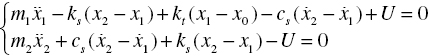
The equations of motion for a quarter-vehicle model shown in Figure 4.3 are written as:
The total damping force of a semi-active suspension can be regarded as the common damping force ![]() plus the controllable damping force U, which can be expressed as:
plus the controllable damping force U, which can be expressed as:
The state variables are:
For simplicity, take x0 = w(t), which represents the road’s speed input as white noise. The state equation of the system can be written as:
Taking the sprung mass acceleration ![]() as the output variable, one has the output equation:
as the output variable, one has the output equation:
where

4.3.2 Integrated Optimization Design of a Semi-active Suspension System
Active and semi-active suspensions have been widely applied and developed in the automotive industry as computers, and electronic and hydraulic servo techniques have improved. At the same time as the development of control theories, plenty of control methods have been applied to active and semi-active suspension systems, such as optimum control, preview control, adaptive control, neural network control and fuzzy logic control. Usually, the optimization theory is first applied to design the mechanical structure parameters of an active or semi-active suspension system. Then, some control strategies are applied to design the controller. These methods divide the procedure of a mechanical control system into two parts. Although both of them are applied to the optimization design process, it’s actually hard for an active or semi-active suspension to reach the desired effect in practice. In fact, from the control point of view, the mechanical structure parameters, which are optimized by just considering motional or static conditions, are not always optimal. In the same way, the control parameters designed by just considering the system’s stability and dynamics are not optimal either. There are complex and coupled relationships between the mechanical structure system and the control system, and this relationship should be considered in order to obtain global optimal parameters. Figure 4.4 gives the concept of an integrated design for a mechanical/control system. As shown in Figure 4.4, the control target and the control system are interrelated. It is more reasonable to optimize the two systems at the same time rather than to do optimization separately in order to get better results[3].

Figure 4.4 The integrated design of the controlled target and the control system.
Thus, traditional design methods cannot coordinate the performance between the mechanical and the control systems. It is not a global optimal design, and it is necessary to use a global optimal design which considers both the mechanical structure parameters and the control parameters in order to get the ideal performance from a system.
The integrated design of the mechanical structure parameters and the control parameters started from the late 1980s and early 1990s of last century. For example, Japanese scholar Asada proposed an integrated optimization method of mechanical structure parameters and control parameters about single-link and two-link manipulators successively[4–5]; American scholar Anton adopted the approach of recursive experiments to integrated optimization of the mechanical structure and control parameters[6]. The stability and robustness study about the integrated optimization methods of the structure and control parameters has been done by Alexander, Savant, Shi and other scholars[7–10]. Here, based on a semi-active suspension system, one would be aimed at doing some exploratory work about the integrated optimization design of the structure and control parameters for engineering applications.
4.3.3 The Realization of the Integrated Optimization Method[11–12]
As shown in Figure 4.5, this optimization method adopts a cyclic structure, mainly due to the need to estimate whether the mechanical structure parameters and control parameters of the system are optimized simultaneously. If the optimal results are not reached, the mechanical structure parameters and control parameters should be modified. Then they should be checked again until both of them reach the best configuration.

Figure 4.5 The basic process of integrated design.
When a vehicle is running, the vibration caused by the road’s roughness excitation is a stochastic and uncertain disturbance, which makes the response characteristics of a suspension system become very complicated. Based on this, the genetic algorithm (GA) and the LQG control method of the integrated optimization design for a suspension system is applied, and the specific steps are as follows:
- Determine the structure parameters, structure models, performance indexes and constraint conditions of a suspension system.
- Initialize the population to optimize the structure parameters by using the genetic algorithm, and to establish the mathematical model of a suspension system.
- Design a controller for the population by using the LQG control strategy, and calculate the fitness values.
- Judge whether the system meet the convergence conditions. If not, recalculate by using the genetic algorithm until it meets the convergence conditions.
- Determine whether to meet the performance indexes of a suspension system. If the conditions are met, determine the structure and control parameters of a suspension system, and end the optimization process. Otherwise, go back to step (1), reinitialize the structure and control parameters of a suspension system and recalculate them.
The structure parameters, models, performance indexes, and constraint conditions of a suspension system depend on specific problems. The details are not shown here. The following sections introduce the mathematical models, the implementation of the genetic algorithm, the design of a LQG controller for a semi-active suspension system, and the simulation results.
4.3.4 Implementation of the Genetic Algorithm
The genetic algorithm assimilates the evolution of the “survival of the fittest” of a natural system, which provides a robust searching method in a complex spatial domain. The genetic algorithm is carried out by using simple calculations, and does not need any restrictive assumptions (such as function continuity, derivative existence, and unimodal, etc.) for the searching space.
For a quarter-vehicle model, if the requirements for riding comfort and driving safety are considered, the performance index function J can be written as
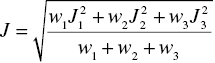
where J1 is the total variance of the body’s vertical acceleration responses; J2 is the total variance of the tyre dynamic load responses; J3 is the total variance of the suspension dynamic travel responses; and w1–w3 are the influence coefficients of each performance index for J.
Let the fitness function f = 1/J. The design goal is to find the parameters which minimize the performance index J and maximize the function f. The structure parameters of a suspension system needing optimization are the suspension stiffness ks, tyre stiffness kt, and unsprung mass m1, as shown in the following steps.
- Parameter coding
A binary code is used where each parameter is coded by a different length respectively, and then the parameters are cascaded to form a chromosome string. For any solving parameter xi, the binary code with k bit length is used, and the upper and lower bound of xi is a and b, respectively. If Mi is the corresponding binary code, the relationship between Mi and xi is as follows:

- Generate the initial population
Use a stochastic method to generate N = 100 individuals as the initial population.
- Selection
Use the roulette method to select; i.e., when the fitness value of the i-th individual of the population is fi, the probability that it selects is
 . The larger the fitness value of the individual, the more the chance of being selected, and vice versa.
 - Crossover
Make the crossover rate Pc = 0.6 and use multiple-point (3 points) crossover. First, match stochastically the individuals of the populations; then set stochastically the crossover point KC1, KC2 and KC3 in each matched individual within a fixed range; finally, the matched individuals exchange information in the corresponding location.
- Mutation
Take a small probability for the mutation probability Pm = 0.1, use a single-point mutation (which means to pick up a part of the individuals stochastically), and then inverse it.
- Assessing the values of fitness functions
If the values of the fitness function of continuing 15 generations do not change, the mutation probability Pm with 10% speed is increased. If the values of the fitness function still do not change for a continuing 5 generations after increasing the mutation probability, then it converges and the genetic algorithm ends; otherwise, turn to step (7).
- Convergence condition
The error of the fitness function Δf = fmax−fmin. When Δf < 0.05, the algorithm converges, and the cycle of the genetic algorithm ends; otherwise, turn to step (3).
4.3.5 LQG Controller Design
Here, the LQG (linear quadratic Gauss) controller based on an observer is used. For the model as shown in equation (4.18), let w(t) as the road speed excitation (white noise that acts on the system), and v(t) as the measurement noise. If these signals are a Gauss process with zero mean, that is:
The LQG optimal problem is to design a control input u and minimize the quadratic performance index:

where Q and R are the weighting matrices for state variables and control variables respectively; Nc is the weighting matrix for the two variables; and tf is the end time.
Generally, equation (4.22) can be simply shown as:

According to the separation theorem and the Kalman filtering principle, the state equation of the optimal estimator can be obtained as follows:
The gain Kl of the filter is:
Here, P satisfies the following Raccati equation:
Then, the estimated state ![]() is used to be substituted into X, and to design the optimal control as:
is used to be substituted into X, and to design the optimal control as:
where
Here, Pc satisfies the following Riccatic algebra equation:
4.3.6 Simulations and Result Analysis
Some parameters for the integrated optimization simulation are shown in Table 4.2. When considering the performance of a suspension system, the values ks ![]() [8000, 18000], kt
[8000, 18000], kt ![]() [80000,180000], m1
[80000,180000], m1 ![]() [30,40], w1= 0.65, w2= 0.25, and w3= 0.1 are taken for the simulation. Assuming a vehicle is running on a level B road with a medium speed v = 20m/s, and the road’s surface roughness coefficient is
[30,40], w1= 0.65, w2= 0.25, and w3= 0.1 are taken for the simulation. Assuming a vehicle is running on a level B road with a medium speed v = 20m/s, and the road’s surface roughness coefficient is ![]() , the root mean square value σ = 0.317(m/s) of the stochastic excitation signals of the road speed can be obtained. Using MATLAB to do the simulation, the results are shown in Table 4.2 and Figures 4.7–4.9.
, the root mean square value σ = 0.317(m/s) of the stochastic excitation signals of the road speed can be obtained. Using MATLAB to do the simulation, the results are shown in Table 4.2 and Figures 4.7–4.9.
Table 4.2 Some physical parameters of the suspension system.
| Structure parameters | ||||
| Before and after optimization |
Sprung mass m2/kg |
Unsprung mass m1/kg |
Suspension stiffness ks/N.m−1 |
Tyre stiffness kt/N.m−1 |
| Before integrated optimization | 300 | 34 | 14000 | 120000 |
| After integrated optimization | 300 | 32 | 15200 | 100670 |
From Table 4.2, it is clear that, after the integrated optimization method, the suspension stiffness ks increases, the tyre stiffness kt significantly decreases and the unsprung mass m1 stays almost unchanged. Theoretically, the unsprung mass has little effect on the riding comfort so, in the integrated optimization process, the unsprung mass m1 need not be the optimal target. The adherence between the tyre and road’s surface can be significantly increased and the driving safety improved through reducing the tyre stiffness kt. The increase of the suspension stiffness ks decreases the suspension dynamic travel and ensures the limit travel.
The stochastic exciting signals of road speed are shown in Figure 4.6. The convergence curves of the evaluation index J are shown in Figure 4.7. In the integrated optimization process of the mechanical structure parameters and control parameters, the evaluation index J converges to a stable minimum value by using the genetic algorithm after a certain number of cycles of selection, crossover, and mutation. From Figure 4.8(a), it is clear that, by using the LQG controller for a semi-active suspension, the integrated optimization system can reduce the acceleration response of the sprung mass and improve the riding comfort, when compared with the non-integrated optimization system (i.e., the semi-active suspension system with given structure parameters to design the LQG controller). As shown in Figures 4.8(b) and (c), riding comfort and driving safety have been increased, and both the tyre and suspension dynamic travel are improved after the integrated optimization control for a semi-active suspension with the LQG controller is implemented. Similarly, from the frequency response curves of the sprung mass acceleration, as shown in Figure 4.9, the acceleration response in the frequency domain 1–50rad/s of the integrated optimization system has improved significantly compared with the non-integrated optimization system. Here the solid line in the figures represents the integrated optimization, and the dotted line represents the non-integrated optimization.

Figure 4.6 Stochastic exciting signals of road speed.
Figure 4.7 Convergence curves of the evaluation index J.

Figure 4.8 Simulation results. (a) Vertical acceleration of the sprung mass. (b) Tyre dynamic load. (c) Suspension dynamic travel. (d) Controlled damper force.

Figure 4.9 Frequency response of the sprung mass’ vertical acceleration.
Table 4.3 compares the data of the tyre dynamic load, body acceleration, suspension dynamic travel, and other indexes of the suspension system under different velocities. Method 1 is the integrated optimization semi-active suspension with the LQG controller, and method 2 is the non-integrated optimization semi-active suspension with the LQG controller. It is obvious that when using method 1 each index is better than when using method 2.
Table 4.3 Comparison of the simulation results (RMS).
| Indexes | Method 1 | Method 2 | ||||
| Velocity |
|
|
|
|
|
|
| v = 20m/s | 168.1779 | 0.8987 | 0.0411 | 344.0955 | 1.7045 | 0.0459 |
| v = 30m/s | 170.5303 | 0.9077 | 0.0634 | 349.2768 | 1.7282 | 0.0741 |
Through the simulation results of the mechanical structure and control parameters of a quarter-vehicle model, it can be seen that the integrated optimization method has a significant effect on improving riding comfort and driving safety. The integrated optimization method effectively reaches the performance of the mechanical structure and the controller and combines them to improve the interaction between them in a traditional optimization process. Thus, the designed suspension system can obtain the global optimum.
4.4 Time-lag Problem and its Control of a Semi-active Suspension[13–14]
The time-lag phenomenon widely exists in vehicle control systems, and is one of the main factors that causes system instability and decreases performance. Due to the great influence on performance in a suspension system, the time-lag problem is one of the hotspot studies of semi-active suspension systems. In addition, time-lag mainly affects the low-frequency characteristics of a suspension system which is more sensitive to the human body. Then again, it will have a strong impact on riding comfort and handling stability. Therefore, it is necessary to consider the time-lag effect on a semi-active suspension system and adopt some measures to weaken the adverse effect of time-lag on a suspension system.
4.4.1 Causes and Impacts of Time-lag
Currently, the active and semi-active suspension systems and other control systems are mainly composed of signal detection devices, controllers, actuators, and controlled objects. The sources of time-lag in a control system are:
- Transmission time-lag of the measured signals from the sensors to the controller;
- Time-lag caused by the calculation of the control law;
- Time-lag of transmitting the control signals to the actuator;
- Time-lag caused by the response time of the actuator;
- Time-lag caused by the time required to establish the control.
It is thus clear that time-lag mainly exists in three steps of the control process. First, it exists in the signal detection channel of a sensor, such as the response time-lag and transmission time-lag of a sensor. Second, it exists in the disturbance channel of a controlled target, for example, the required time that a driver exerts steering wheel angle or steering force until the front wheel starts to turn. Finally, it exists in the control input channel of an actuator, such as the required time from a step motor, direct current motor, solenoid valve and an actuator to receive instructions to start an action. The time-lag in a vehicle system in different locations has different effects on the performance of a control system, and it is necessary to analyze the location of the time-lag effect on a control system.
Supposing that there are different time-lags τ1, τ2 and τ3 in the disturbance channel of a controlled target, the detection channel of the sensor signals, and the control input channel of an actuator respectively. Then, a closed loop control system with pure time-lag is shown in Figure 4.10.

Figure 4.10 Closed loop system with time-lag.
The transfer function GCR(s) and GCL(s) of a closed loop system with the time-lag under the given desired output and the external disturbances can be seen in Figure 4.10.

where GC(s) is the controller’s transfer function; Go (s) is the transfer function of the input channel of the controlled target; H(s) is the transfer function of the sensor measure channel; GL(s) is the transfer function of the disturbance channel of the controlled target; R(t) is the desired output signal of the system; and C(t) is the actual output signal of the system.
Both of their characteristic equations can be expressed as:
From equations (4.30) and (4.31), it is known that the time-lag locations impacting the performance of a control system are as follows.
- The disturbance channel of a controlled target
The pure lag factor
 , which is generated by the time-lag τ1 that exists in the disturbance channel of a controlled target, appears in the numerator of the transfer function GCL(s). Compared with a no-lag control process, the control output C(t) under the action of the external disturbance L(t) will need to delay a pure lag time τ1. Because the characteristic equation (4.31) of a closed-loop system does not contain the pure lag factor
  , the time-lag τ1 of the disturbance channel has no influence on the stability of the control system. This makes the control output C(t) of the whole transient process of the control system delay a pure-lag time τ1.
 - The detection signal channel of sensors
The time-lag τ2 that exists in the detection channel of sensors appears in the characteristic equation (4.31). It affects the stability of the control system but has no influence on the real-time value of the control output C(t).
- The control input channel of an actuator
The pure lag factor
 which is generated by the time-lag τ3 of the input channel of an actuator not only affects the stability of a closed-loop system, but it also makes the output C(t) delay a pure lag τ3.
 - All three channels
If the control input channel, signal detection channel, and other links of the closed-loop system have a time-lag, then the pure lag factor will appear in the characteristic equations of a closed-loop system. In addition, the time-lag of two channels has an influence of a pure lag additive action on the stability of the closed-loop system.
It is thus clear that although the time-lag in the disturbance channel of the controlled target does not affect the system stability, it has great relevance with the real-time display of the output signals of the system. When time-lag exists in the control input channel and signal detection channel of a chassis control system, the stability of the closed-loop system is affected by the total lag (
 ) of adding both lags. Therefore, in the vehicle control process, it is necessary to compensate or control the time-lag of each link, to weaken the negative impact on the control performance, and to avoid the unexpected instability of the system.
4.4.2 Time-lag Variable Structure Control of an MR (Magneto-Rheological) Semi-active Suspension
For a semi-active suspension system, Magneto-rheological Semi-active Suspension (MSAS) has been extensively studied and has certain applications. It uses MR dampers as actuators to change the values of the damping force. The control system adjusts the exciting current that is given to the magnetic coil in the damper according to the road’s surface excitation and suspension status, so as to change the magnetic field intensity of the coil. It also makes the apparent viscosity of the Magneto Rheological Fluid (MRF) in the damping channel change. Thus, continuous adjustment of the damping force can be achieved. The response process of the MSAS involves measuring the vehicle status and road signals, calculating the control effect and achieving the controllable damping force. This will generate a larger time-lag, impacting the control performance of the system if the response time is longer in some links. At present, these methods are used to solve the time-lag impact on the control performance of a semi-active suspension system:
- Smith pre-evaluation compensation method. In the control channel with pure lag of the system, a parallel compensator is used to eliminate the effect of pure lag to the control process.
- Critical time-lag values of the control system are calculated to eliminate the effect of time-lag by using time delay feedback links.
- The controller is designed directly from the dynamic equations with time-lag.
Although the first and second methods can improve the effect of the time-lag, they mainly compensate for the time-lag after the controller has been designed. Because they do not consider the effect of time-lag in controller design, it’s hard to ensure the stability of the control system.
The third method is used first to build up the dynamic equations with time-lag, then the effect of time-lag in controller design is considered in advance, so it is generally suitable and easy to ensure the stability of the control system. Thus, it is the main method used to solve the time-lag nowadays.
4.4.2.1 Time-lag test for an MR damper
As a key component of an MSAS system, the performance of an MR damper can directly affect the control performance of a semi-active suspension. The dynamic performance of an MR damper not only includes the maximal damping force, the maximal travel, and controllable range of the damping force, but also the dynamic response time of the MR damper. Here, the dynamic response time for a self-developed MR damper is tested, so reference to the control strategy design of a semi-active suspension with time-lag is provided.
The identification methods of time-lag include: putting a step signal to the input end of the target with time-lag, then start timing from the moment the step signal is added in, and to end timing when the responses from the output of the target with time-lag can be observed. This period of time τ is the time-lag of the target. According to this identification method, the self-developed MR damper (as shown in Figure 4.11(a)) is tested, with an amplitude of 25mm and frequency of 0.04Hz with the sine wave load by using the MR damper rig (Figure 4.11(b)). Here, the piston rod of the MR damper is in constant motion with a speed of 4mm/s. In the stretching travel of the damper, the transient current is among 0–0.5, 0–1.0, 0–1.5, 0–2.0 A. In the test, it takes the transient process from one steady state of the damping force to another, which is caused by the transient current. The test results under different transient current conditions are shown in Figure 4.12.

Figure 4.11 MR damper and the test rig. (a) Self-developed MR damper. (b) Test rig for an MR damper.

Figure 4.12 Response time of MR damper under different transient current conditions.
By the tests results shown in Figure 4.12, a time-lag table of the MR damper can be obtained. Table 4.4 shows that the response lag of an MR damper has the following characteristics:
- The dynamic response time of an MR damper is less affected by the transient range of the current.
- The response time when the transient current increases is significantly less than when it decreases. This is mainly caused by the remanence in the magnetic circuit of the MR damper, and the rapid decline of the damping force is blocked by the remanence field.
- The response lag of the MR damper is no more than 28ms, and it has a faster dynamic response speed. In order to further improve the performance of the control system, the effect of time-lag in control strategy design should be considered.
Table 4.4 The time-lag of the MR damper with transient current.
| The range of transient current | ||||||||
| Response lag | 0–0.5A | 0–1.0A | 0–1.5A | 0–2.0A | 0.5–0A | 1.0–0A | 1.5–0A | 2.0–0A |
| τ/ms | 20.7 | 22.4 | 20.3 | 21.6 | 26.4 | 25.6 | 27.7 | 26.3 |
4.4.2.2 MSAS model
According to the nonlinear Bingham model and the measured results of the indicator diagram of an MR damper, the following mathematical model describes the characteristics of an MR damper:

where F(t) is the damping force of the MR damper; cs is the viscous damping coefficient; sgn is the sign function; FMR(t) is the coulomb damping force; v is the velocity of the piston rod; ā1, ā2, ā3 are experimental constants (![]() ); and I is the current of the MR damper coil.
); and I is the current of the MR damper coil.
With the development of modern computer technologies and high-performance microprocessors, the time-lag generated by the signal measuring, processing, and control law calculation is very small. So, the response lag of an MR damper is considered, and a 2-DOF quarter car model of a semi-active suspension with the MR lag is built, similar to equation (4.18).
The dynamic equations are:

The parameters in the equations have the same meaning as in equation (4.18).
Defining ![]() as the state variables of the system, the output variables are
as the state variables of the system, the output variables are ![]() ,
, ![]() ,
, ![]() . Thus, the state equation and output equation can be derived as:
. Thus, the state equation and output equation can be derived as:

where


4.4.2.3 Designing a variable structure controller with time-lag
In the above-mentioned modeling process, there is a time-lag τ in the control input channel u(t) of the control system (4.34) for considering the response lag of an MR damper. The time-lag existing in the control input channel will affect the control effect of the entire MSAS and even make the system unsteady. In order to overcome the time-lag problem, an effective treatment is to consider the control input lag when the controller is designed. The goal is to design a controller which not only can make the closed-loop system steady, but can also make the system reach the expected performance when there is a time-lag.
Sliding mode control (SMC) is a nonlinear control method which differs with conventional control methods due to the inherent discontinuity of control. It uses a special sliding mode control method and makes the system’s state move along a sliding surface by switching the control variables in order to reach the expected target. Thus, the sliding mode surface has an indifference to the parameter perturbation of the system and external disturbances. The SMC method is used to design an MSAS controller with its control input being the time-lag. The stability analysis and critical lag calculation of an MSAS with time-lag is carried out in the following section.
- Sliding mode of system
There is a control input lag in the equation (4.34) which increases the difficulty of designing a sliding mode. When the switching is carried out, in order to make the error smaller and avoid serious chattering phenomenon, the switching functionality is constructed as follows:
(4.35)
G is the constant 1 × 4 matrix which meets the condition that the inverse of matrix GB exists. It is obvious then that matrix G exists. Γ is a sliding mode compensator, and has the following mathematical model:
(4.36)
Here, K is the unknown constant 1 × 4 matrix which is related to the input lag τ. Under the condition that the generalized sliding mode condition ss&c.dotab; < 0. is satisfied, one can use the exponential approach law to improve the dynamic quality of the motion, and obtain the derivative of s with respect to time by using a saturation function to replace the sign function, which can be expressed as:
(4.37)
where
 is the approaching velocity;
  is the reaching velocity; and fsat(s) is the saturation function.
The equivalent SMC law can be obtained from the following:
The system’s trajectory reaches the sliding manifold under control law (4.38), the sliding model equation of motion on the sliding manifold is:
where

- Judging the system’s stability
- Critical time-lag of system stability
Applying the theorem stated above, the maximum permissible lag of the MSAS can be gained, which is the critical time-lag
 of the system keeping it steady. It can be obtained by solving the following optimization problem:
In reference[13], the optimization problem (4.42) can also be transformed into the following problem to minimize the generalized eigenvalues.
Using the solver gevp in MATLAB LMI toolbox to obtain the optimization formula (4.43), a globally optimal solution σ* would be reached. Then, the critical time-lag
 of the MSAS can be obtained.


4.4.3 Simulation Results and Analysis
By using the SMC (named controller I) with the time-lag, the MSAS simulation mentioned before is carried out. The results are compared with the traditional SMC (named controller II) without the time-lag. Some parameters used in the simulation are shown in Table 4.5.
Table 4.5 Simulation parameters.
| Parameters | Values | Unit |
| ks | 20 | kN.m–1 |
| kt | 180 | kN.m–1 |
| m2 | 320 | kg |
| m1 | 40 | kg |
| cs | 1317 | N.s.m–1 |
| ā1 | 18.98 | / |
| ā2 | 51.22 | / |
| ā3 | 314.77 | / |
In order to make the system’s state trajectory reach the sliding mode surface quickly and without a large chatter, the parameters ![]() ,
, ![]() are selected after repeating the adjustment. Thus, the critical time-lag
are selected after repeating the adjustment. Thus, the critical time-lag ![]() = 32ms is reached by solving equation (4.43), which is close to the actual time-lag (<28ms) of the MR damper tested before. The value of K = (–198.14 182.06 19.87 –3.67) can also be obtained by the solver feasp. To make sure that GB is reversible after repeatedly doing adjustments, G = (14.28 –1.25 0 –35.6) is determined. Then, the actual control effect of the MSAS is better.
= 32ms is reached by solving equation (4.43), which is close to the actual time-lag (<28ms) of the MR damper tested before. The value of K = (–198.14 182.06 19.87 –3.67) can also be obtained by the solver feasp. To make sure that GB is reversible after repeatedly doing adjustments, G = (14.28 –1.25 0 –35.6) is determined. Then, the actual control effect of the MSAS is better.
4.4.3.1 Simulation of the bump road input
Assume a vehicle is running along a bump road at a speed of 30 km/h. The length of the bumb is 0.1m, and the height is 0.06m. The mathematical model of the bump road can be described by the following equation:

where ã is the bump height; l is the bump length; uc is the vehicle speed.
The simulation curves of the body vertical acceleration, suspension dynamic deflection, and tyre dynamic load by using controller I and II, and the passive suspension under the bump road excitation conditions, are shown in Figures 4.13–4.15. The specific simulation results are shown in Table 4.6. As shown in the figures and table, by using controller I, the peak responses of the body acceleration, suspension dynamic deflection, and tyre dynamic displacement are improved by 56.15%, 38.71% and 26.9% respectively, compared with the passive suspension. As well, the settling time of the transient process is shorter. The peak values of the controller II without considering time-lag improved by 25.02%, 20.04%, 23.35% respectively, compared with the passive suspension. Due to a 28ms time-lag in the control channel, it will be out-of-step with the control in the simulation.
Figure 4.13 Body vertical acceleration.


Figure 4.15 Tyre dynamic displacement.
Table 4.6 Simulation results of a bump road input.
| Parameters | Control methods | Peak responses | Settling time t/s |
| Body vertical acceleration |
Passive suspension | 10.43 | 1.52 |
| Controller I | 5.02 | 0.37 | |
| Controller II | 8.57 | 0.68 | |
|
Suspension dynamic deflection |
Passive suspension | 10.23 | 1.78 |
| Controller I | 6.27 | 1.15 | |
| Controller II | 8.18 | 1.43 | |
| Tyre dynamic displacement |
Passive suspension | 1.97 | 1.68 |
| Controller I | 1.44 | 0.45 | |
| Controller II | 1.51 | 0.72 |
4.4.3.2 Simulation of the road’s surface stochastic input
Assume a vehicle is running along a grade B road at a uniform speed of 70km/h, and the filtering white noise is the stochastic road input. The road’s roughness coefficient is ![]() m3/cycle, and the low cut-off frequency is 0.1Hz. The simulation results of three different modes of stochastic road’s surface are shown in Figures 4.16–4.18.
m3/cycle, and the low cut-off frequency is 0.1Hz. The simulation results of three different modes of stochastic road’s surface are shown in Figures 4.16–4.18.

Figure 4.16 Body vertical acceleration.
Figure 4.16 shows that the optimal damper force calculated by controller II cannot be achieved in real time, due to the 28ms time-lag in the control channel. Therefore, it is difficult to reduce vehicle vibration. The response lag of the MR damper of the controller I is considered in advanced, and the input time-lag in the MSAS control channel is compensated reasonably, such that the body vertical acceleration is restrained effectively.
In Figure 4.17, controller I makes the suspension dynamic deflection achieve a better effect compared with controller II, when the time-lag is considered.
Figure 4.17 Suspension dynamic deflection.
In Figure 4.18, it is clear to see that the time-lag has a greater effect on the body vibration. Controller I makes the peak values of the first resonance decrease by 44.16% at 28ms lag, compared with the passive suspension; controller II makes the peak values of the first resonance decrease by 18.18%. This is consistent with the simulation results of the bump input. It is obvious that the existence of time-lag greatly influences the ride comfort.

Figure 4.18 Amplitude-frequency characteristics of the body acceleration.
In order to analyze the influence of the control effect under different control input lag, through changing time-lags in simulations, the root mean square (RMS) values of the body vertical acceleration, suspension dynamic deflection, and tyre dynamic displacement are obtained under different time-lags, as shown in Table 4.7 and Table 4.8.
Table 4.7 RMS values of vehicle response by controller I.
|
Time-lag τ/ms |
Body acceleration |
Suspension dynamic deflection |
Tyre dynamic displacement |
| 0 | 0.374 | 0.656 | 0.192 |
| 5 | 0.403 | 0.685 | 0.198 |
| 10 | 0.421 | 0.711 | 0.204 |
| 15 | 0.458 | 0.741 | 0.207 |
| 20 | 0.492 | 0.780 | 0.213 |
| 25 | 0.507 | 0.787 | 0.219 |
| 30 | 0.514 | 0.225 | 0.225 |
| 35 | 0.856 | 1.007 | 0.349 |
| 40 | 1.545 | 1.137 | 0.408 |
| 45 | 2.793 | 1.392 | 0.577 |
Table 4.8 RMS values of the vehicle response by controller II.
| Time-lag τ/ms | Body acceleration |
Suspension dynamic deflection |
Tyre dynamic displacement |
| 0 | 0.353 | 0.637 | 0.178 |
| 5 | 0.423 | 0.721 | 0.204 |
| 10 | 0.472 | 0.777 | 0.216 |
| 15 | 0.591 | 0.803 | 0.217 |
| 20 | 0.714 | 0.821 | 0.224 |
| 25 | 0.911 | 0.935 | 0.315 |
| 30 | 1.209 | 0.910 | 0.331 |
| 35 | 1.515 | 1.118 | 0.352 |
| 40 | 1.883 | 1.469 | 0.497 |
| 45 | 3.661 | 1.988 | 0.612 |
In Table 4.7 and Table 4.8, the RMS values of the body vertical acceleration, suspension dynamic deflection, and tyre dynamic displacement, obtained by using controller I and controller II, are increased gradually with the increase of the time-lag in the control input channel. But controller II increases more, and this leads to controller II being unstable and divergent when the time-lag gets larger. This reflects that the control quality rapidly deteriorates with the increase of the time-lag in the control input channel.
4.4.4 Experiment Validation
To verify the validity of the control strategy, an experimental study is performed on a 4-channel vibration rig with a car implementing the MSAS. The experimental setup is shown in Figure 4.19. Several cases were tested in the experiments. Controller I and controller II separately considered two types of road inputs (bump road and stochastic road), and the results are compared with those from the passive suspension. The vehicle parameters used in the tests are almost the same as with the simulation data.

Figure 4.19 Experimental setup.
The test results of the bump road input are shown in Figure 4.20. The peak values of the body vertical acceleration decrease from 11.6m/s2 to 4.98 m/s2.The peak values of the tyre dynamic load decrease remarkably and the settling time significantly shortens. These results are gained under the conditions of the bump road input and carried out by controller I, in which the time-lag is considered. For body vertical acceleration and tyre dynamic load carried out by controller II (without time-lag), the improved effect is less evident compared with controller I. The results show that the time-lag has a great influence on the control quality of the system, and simulations come up with the same conclusions.

Figure 4.20 Experimental results of a bump road input. (a) Body acceleration. (b) Tyre dynamic load.
Under stochastic road inputs with an amplitude of 10mm, and a signal bandwidth of 0.1–20Hz, the test results are shown in Table 4.9.
Table 4.9 RMS values comparison between simulation and experiment results.
| Body acceleration |
Tyre dynamic load Fd /KN | |||
| Control mode | Experiment results | Simulation results | Experiment results | Simulation results |
| Controller I | 0.46 | 0.51 | 0.427 | 0.484 |
| Controller II | 0.77 | 0.83 | 0.512 | 0.575 |
| Passive suspension | 0.89 | 1.02 | 0.584 | 0.606 |
From Table 4.9, it is clear that the RMS value of the body acceleration is reduced from 0.89m/s2 to 0.46m/s2 by using controller I. Compared with the passive suspension, it is improved by 48.3%, and the RMS value of the tyre dynamic load is reduced from 0.704KN to 0.427KN, which is improved by 26.9%. By using controller II, the RMS value of the tyre dynamic load is improved by only 12.3%, as the time-lag leads to it being out-of-step with the control. The experimental results are close to the simulation results, which fully verify that the stability of the MSAS can be improved further by using the sliding mode control method and considering time-lag. It also shows that the lag influence on the control quality can be reduced, and good vibration performance of the MSAS can be obtained.
Of course, this method can be applied to other control systems of vehicles with time-lag, due to the SMC strategy considering the influences of time-lag. In addition, this method starts directly from the time-lag equations of motion of the system, and thus can be widely used.
4.5 Design of an Active Suspension System[15–16]
Many advances have been made in active suspension and control theory nowadays. There are many control strategies for a 7-DOF full-vehicle model and a 4-DOF half-vehicle model, such as H∞ control, H2 control, L2 control, adaptive control, and optimal control. Generally speaking, H∞ control strategy can solve the robust stability problem of a controlled target, and H2 control strategy lets the controlled targets have a better dynamic performance. Combining H2/H∞ to build a hybrid control strategy, the problems of robust stability and optimal dynamic performance of a controlled target can be solved with better results. For a half-vehicle model, the riding comfort is related to the body vertical acceleration, pitching angular acceleration, and suspension dynamic deflection. The handling stability is related to the front and rear tyre dynamic loads. Based upon this consideration, and also considering how to reduce the complexity of a controller, a multi-objective optimization control strategy for an active suspension system is introduced in this section. Choosing H∞ norm as the robust performance index of a high-order unmodeled, H2 norm as the time-domain LQG performance index of perturbation action, and choosing weighting matrices to set the frequency-domain performance index of a suspension system, a multi-objective H2/H∞ hybrid controller based on LMI (Linear Matrix Inequality) is designed. Simulation results show that the performance indexes by using the multi-objective H2/H∞ hybrid control method under the premise of the system with unmodeled robust stability, the handling stability and riding comfort of a vehicle can be improved effectively compared with the H2 control or H∞ control.
4.5.1 The Dynamic Model of an Active Suspension System
The 12-order state equation of a half-vehicle model of an active suspension, as shown in Figure 4.21, can be represented as:
and the state variables are:
the control variables are:
the disturbance variables are:
where ![]() is the body vertical velocity,
is the body vertical velocity, ![]() is the pitching angle,
is the pitching angle, ![]() ,
, ![]() are the front and rear suspension dynamic deflections respectively,
are the front and rear suspension dynamic deflections respectively, ![]() ,
, ![]() are the front and rear vertical velocities respectively,
are the front and rear vertical velocities respectively, ![]() ,
, ![]() are the front and rear tyre dynamic displacements respectively, q1, q2 are the hydroelectric velocities of the front and rear servo-valves respectively, and v1, v2 are the hydroelectric volume of the front and rear servo-valves respectively. The control input
are the front and rear tyre dynamic displacements respectively, q1, q2 are the hydroelectric velocities of the front and rear servo-valves respectively, and v1, v2 are the hydroelectric volume of the front and rear servo-valves respectively. The control input ![]() is the current of the front and rear servo-valves. The disturbance
is the current of the front and rear servo-valves. The disturbance ![]() is the road’s surface speed excitation of the front and rear tyres and handling torque respectively.
is the road’s surface speed excitation of the front and rear tyres and handling torque respectively.

Figure 4.21 Half-vehicle model of an active suspension.
4.5.2 Design of the Control Scheme
An active suspension system with an uncertainty of high-order unmodeled is considered, as shown in Figure 4.22.

Figure 4.22 Diagram of controlled target.
In Figure 4.22, we are measuring the output y = ![]() ; control input
; control input ![]() ; performance evaluation
; performance evaluation ![]() ; and road disturbance input
; and road disturbance input ![]() .
.
Here, G0(s) is a nominal active suspension model of a 4-DOF half-vehicle, and a real model is ![]() , when the uncertainty Δ of the dynamic unmodeled is considered.
, when the uncertainty Δ of the dynamic unmodeled is considered.
Assuming ![]() ; where Δ1(s) is the high-order unmodeled part of a servo-valve attached to the front suspension, and Δ2(s) is the high-order unmodeled part of a servo-valve attached to the rear suspension. According to reference [15], the upper bound functions of Δ1(s) and Δ2(s) are
; where Δ1(s) is the high-order unmodeled part of a servo-valve attached to the front suspension, and Δ2(s) is the high-order unmodeled part of a servo-valve attached to the rear suspension. According to reference [15], the upper bound functions of Δ1(s) and Δ2(s) are

The weighting coefficient matrix Sw is introduced to improve the system robustness of anti-disturbance, the weighting coefficient matrix Sz and the weighting function matrix W1(s) are introduced to improve the evaluation index z of the system. Considering that the system has a maximum uncertainty of ![]() , so as to enhance the robustness of dynamic unmodeled part. For the unmodeled part Δ(s), let
, so as to enhance the robustness of dynamic unmodeled part. For the unmodeled part Δ(s), let ![]() ,
, ![]() ,
, ![]() ,
, ![]() , and the weighting function matrix
, and the weighting function matrix ![]() . Thus, the weighting function of the body vertical acceleration is W11(s), and the weighting function of the pitching angular acceleration is W12(s).
. Thus, the weighting function of the body vertical acceleration is W11(s), and the weighting function of the pitching angular acceleration is W12(s).
The human body is most sensitive to vertical vibration in the frequency range from 4Hz to 12.5Hz, and to horizontal vibration in the frequency range from 0.5Hz to 2Hz, according to the ISO2631-1(1997). Therefore, we choose  to increase the weight of the vertical vibrations in the 4~12.5Hz zone, and
  to increase the weight of the horizontal vibrations in the 0.5~2Hz zone. In addition, we choose a weighting coefficient matrix as follows:
The control system of the generalized controlled target is shown in Figure 4.23, and the simplified form is shown in Figure 4.24.
The transfer function of the generalized controlled target is:

Figure 4.23 Control block diagram of the generalized controlled target.

Figure 4.24 Simplified block diagram of the control system.
From Figures 4.23 and 4.24, the state equations of a generalized controlled target can be obtained.

where ![]() ,
, ![]() ,
, ![]() , xg are the state variables of a generalized controlled target, and A, B1, B2, C1, C2, C3, D11, D12, D21, D22, D3 are the coefficient matrices.
, xg are the state variables of a generalized controlled target, and A, B1, B2, C1, C2, C3, D11, D12, D21, D22, D3 are the coefficient matrices.
Channel Tqp: The transfer function from p to q. Consider the disturbance of p, which is generated by the uncertain link Δm(s), and use the H∞ norm to evaluate Tqp to get better robustness.
Channel ![]() : The transfer function from w to
: The transfer function from w to ![]() . Consider the road disturbance w, which is a stochastic white noise signal, and use the H2 norm to evaluate
. Consider the road disturbance w, which is a stochastic white noise signal, and use the H2 norm to evaluate ![]() to get a better dynamic performance index.
to get a better dynamic performance index.
4.5.3 Multi-objective Mixed H2/H∞ Control
Design the output feedback controller K(s) for a generalized controlled target. The equations of the controller K(s) are:

The transfer function matrix of the controller is:

The control inputs are:

Design the controller to solve the matrices K, L, M and N.
- Two control schemes of a multi-objective mixed H2 /H∞ control
Control scheme I: Design an output feedback controller to satisfy the following conditions:
- The closed-loop system is stable;
 ;
;
Control scheme II: Design an output feedback controller to satisfy the following conditions:
- The closed-loop system is stable;


Adjust the weights of the norm of the two channels
 Tqp and
  in the H2/H∞ mixed control, and to satisfy the condition:
  , so that a better performance of robust stability and dynamic performance can be obtained.
 - Mixed control algorithm of H2 /H∞
The mixed control algorithm of H2 /H∞ based on LMI can be expressed as:
- The suboptimal control problem of H2/H∞ is solvable if and only if there are symmetric matrices X, Y, Z, and meet the condition that
 and the following three LMIs:


- There are full column rank matrices U and V, and make
 ,
,  and
and  ,
, 
- There is a
 , and
, and 

- The coefficient matrix of equation (4.52) is:

- The suboptimal control problem of H2/H∞ is solvable if and only if there are symmetric matrices X, Y, Z, and meet the condition that
4.5.4 Simulation Study
Take a1 = 1, a2 = 1 in simulation. In control scheme I, suppose that ![]() = 0.7, thus, min
= 0.7, thus, min ![]() = 0.952 can be obtained. Then, take a = 0.5, b = 0.5, m1 = 1, n1 = 1 in the control scheme II, thus,
= 0.952 can be obtained. Then, take a = 0.5, b = 0.5, m1 = 1, n1 = 1 in the control scheme II, thus, ![]() = 0.657 and
= 0.657 and ![]() = 0.483 can be obtained. ass1, ass2, ass3, ass4 and pss denote the H∞ control, H2 control, multi-objective mixed H2/H∞ control scheme I, and control scheme II, and passive suspension respectively. Figures 4.25–4.28 are the response curves under the disturbance which is the given pulse signal excitation at a vehicle speed of 10km/h, and a pulse signal amplitude of 0.06. In Figures 4.25 and 4.26, the performance curves obtained by scheme II are small, and the convergence speed is fast. Thus, the overall performance indexes are better. In Figures 4.27 and 4.28, compared with the passive suspension system, the dynamic deflections of the front and rear suspensions by using H∞ control, H2 control, and control scheme II are dropped considerably. In Figure 4.27, the peak values of the front suspension deflection from large to small are pss, ass4, ass1, and ass2 control strategy. In Figure 4.28, the peak values of the rear suspension deflection, from large to small, are: pss, ass4, ass1, and ass2 control strategy. But the curves of multi-objective mixed H2/H∞ control scheme II have a fast convergence speed and smaller oscillations overall. Figures 4.29 and 4.30 give the response curves under the excitation of a random white noise. The white noise has zero mean and a variance of 0.01. Under the excitation of white noise, the vertical acceleration of the car’s body and the pitching angular acceleration can obtain a better control effect using the control scheme II. It is clear to see from Figure 4.31 that the control scheme II can greatly reduce the gain of the vertical acceleration from the front tyre to the center of the body mass in the frequency range of 4–12Hz. In Figure 4.32, the control scheme II can greatly reduce the gain of the pitching angular acceleration from the front tyre to the body in the frequency range of 1–2Hz. In Figures 4.33 and 4.34, the gains of the front and rear suspension dynamic deflections, from large to small, are: passive suspension, H2 control, control scheme II, and control scheme I, respectively. In Figures 4.35 and 4.36, the front and rear tyre dynamic loads, from large to small, are: passive suspension, H2 control, control scheme I, and control scheme II, respectively. It is clear that control scheme II can obtain a better vehicle handling stability.
= 0.483 can be obtained. ass1, ass2, ass3, ass4 and pss denote the H∞ control, H2 control, multi-objective mixed H2/H∞ control scheme I, and control scheme II, and passive suspension respectively. Figures 4.25–4.28 are the response curves under the disturbance which is the given pulse signal excitation at a vehicle speed of 10km/h, and a pulse signal amplitude of 0.06. In Figures 4.25 and 4.26, the performance curves obtained by scheme II are small, and the convergence speed is fast. Thus, the overall performance indexes are better. In Figures 4.27 and 4.28, compared with the passive suspension system, the dynamic deflections of the front and rear suspensions by using H∞ control, H2 control, and control scheme II are dropped considerably. In Figure 4.27, the peak values of the front suspension deflection from large to small are pss, ass4, ass1, and ass2 control strategy. In Figure 4.28, the peak values of the rear suspension deflection, from large to small, are: pss, ass4, ass1, and ass2 control strategy. But the curves of multi-objective mixed H2/H∞ control scheme II have a fast convergence speed and smaller oscillations overall. Figures 4.29 and 4.30 give the response curves under the excitation of a random white noise. The white noise has zero mean and a variance of 0.01. Under the excitation of white noise, the vertical acceleration of the car’s body and the pitching angular acceleration can obtain a better control effect using the control scheme II. It is clear to see from Figure 4.31 that the control scheme II can greatly reduce the gain of the vertical acceleration from the front tyre to the center of the body mass in the frequency range of 4–12Hz. In Figure 4.32, the control scheme II can greatly reduce the gain of the pitching angular acceleration from the front tyre to the body in the frequency range of 1–2Hz. In Figures 4.33 and 4.34, the gains of the front and rear suspension dynamic deflections, from large to small, are: passive suspension, H2 control, control scheme II, and control scheme I, respectively. In Figures 4.35 and 4.36, the front and rear tyre dynamic loads, from large to small, are: passive suspension, H2 control, control scheme I, and control scheme II, respectively. It is clear that control scheme II can obtain a better vehicle handling stability.

Figure 4.25 Vertical acceleration responses.

Figure 4.26 Pitching angular acceleration responses.

Figure 4.27 Responses of the front suspension dynamic deflection.

Figure 4.28 Responses of the rear suspension dynamic deflection.

Figure 4.29 Vertical acceleration responses of the center of mass.
Figure 4.30 Pitching angular acceleration response of the center of mass.

Figure 4.31 Amplitude-frequency characteristics of the transfer function of the vertical acceleration from the front tyre-road to the center of mass.

Figure 4.32 Amplitude-frequency characteristics of the transfer function of the pitching angular acceleration from the front tyre-road to the center of mass.

Figure 4.33 Amplitude-frequency characteristics of the transfer function of the front suspension deflection from the front tyre-road input.

Figure 4.34 Amplitude-frequency characteristics of the transfer function of the rear suspension deflection from the rear tyre-road input.

Figure 4.35 Front tyre dynamic load.

Figure 4.36 Rear tyre dynamic load.
4.6 Order-reduction Study of an Active Suspension Controller[17–19]
In order to improve vehicle riding comfort and handling stability, various advanced control strategies have been used for the design of active suspension control systems in recent years. The orders of an active suspension model can be more than 20 according to different degrees of freedom. Considering the human sensitivity frequency range, the orders of a generalized system by using weighting frequencies will be higher, and the orders of a controller by using H∞, H2, LQG strategies, etc., will be higher than a generalized system. A high order controller brings great difficulty to engineering applications, increases the complexity, and reduces the real-time and reliability of a control system.
Thus, reducing the orders of a controller as much as possible under the conditions of keeping the performance of a closed loop control system is still unknown. There are usually two kinds of research methods investigating this aspect: one method is to reduce the order of a high order controlled target and design a controller according to the reduction model; the second is to reduce the order of a designed high order controller, such as by using the controller reduction method based on LMI to design a low order controller of an active suspension system. This section introduces how to design an H∞ controller based on a 7-DOF full vehicle model, and design a controller by the Optimal Hankel-norm Reduction (OHNR) method. It shows that the Hankel reduction method can reach a better control effect compared with the other two kinds of reduction methods.
4.6.1 Full Vehicle Model with 7 Degrees of Freedom
Figure 4.37 is a full vehicle model with 7 degrees of freedom, which considers the vertical, pitch, and roll motion of a sprung mass and the vertical motion of non-sprung mass.

Figure 4.37 Diagram of a 7-DOF full vehicle model.
The vertical motion equation of the center of body mass is:

The body pitching motion equation is:

The body roll motion equation is:

The vertical motion equations of four non-sprung masses are:
The state variables of the system are:
The disturbance input is:
The control input is:
The system output is:
The measuring output is:

The state space model of an active suspension system is:

Take ![]() . This model is the minimal realization model of a state space with 14 orders. The corresponding state space model of a passive suspension system is:
. This model is the minimal realization model of a state space with 14 orders. The corresponding state space model of a passive suspension system is:
4.6.2 Controller Design
In the design of an H∞ output feedback controller for the target G0(s), the diagram of the output feedback of a closed-loop control system is shown in Figure 4.38.

Figure 4.38 H ∞ output feedback.
The goal of H∞ control is to design a controller K(s), which can make the interior of a closed-loop system stable and minimize ![]() , where Tzw(s) is the transfer function from the disturbance input w to the controlled output z.
, where Tzw(s) is the transfer function from the disturbance input w to the controlled output z.
Since,

Thus,
The weighting transfer functions are:
 (vertical motion direction)
 (horizontal motion direction)
The weighting transfer function matrix of the controlled output is:
The weighting coefficient matrix of the disturbance input is:
The weighting coefficient matrix of the controlled output is:
The diagram of the H∞ weighted control is shown in Figure 4.39.

Figure 4.39 H ∞ weighted control.
According to the ![]() control theory, in order to effectively suppress the disturbance input, it should have
control theory, in order to effectively suppress the disturbance input, it should have ![]() to reach the minimum. Now the controller design problem can be converted into the
to reach the minimum. Now the controller design problem can be converted into the ![]() standard design containing the weighting function of a generalized system. By using the MATLAB/LMI toolbox, the controller
standard design containing the weighting function of a generalized system. By using the MATLAB/LMI toolbox, the controller ![]() can be solved.
can be solved.
4.6.3 Controller Order-reduction
4.6.3.1 Application of the Optimal Hankel-norm Reduction (OHNR) Method
By calculations, the order of the ![]() controller K(s) is 20, K(s) is stable, and (Ak, Bk, Ck, Dk) is the minimal realization of K(s). Thus, the reduction order controller Gi(s) can be obtained as follows by selecting the orders of the controller K(s) from order 5 to 10. The results are shown in Table 4.10.
controller K(s) is 20, K(s) is stable, and (Ak, Bk, Ck, Dk) is the minimal realization of K(s). Thus, the reduction order controller Gi(s) can be obtained as follows by selecting the orders of the controller K(s) from order 5 to 10. The results are shown in Table 4.10.
Table 4.10 Comparison of the OHNR results of a 20 order ![]() controller.
controller.
| The order of controller i |
|

|
|

|
|
|
|
|
| 10 | 360.4 | 4.8% | 438.1 | 3.1% | 0.8503 | 3.1% | 83796 | 34.6% |
| 9 | 817.6 | 10.8% | 1019.9 | 7.3% | 0.8434 | 2.3% | 56810 | –8.7% |
| 8 | 1267.5 | 16.8% | 2257.5 | 16.1% | 0.8629 | 4.6% | 100640 | 61.7% |
| 7 | 1373.6 | 18.2% | 2454.9 | 17.5% | 0.8666 | 5.1% | 118900 | 91.0% |
| 6 | 1540.7 | 20.4% | 2031.1 | 14.4% | 0.8479 | 2.8% | 85922 | 38.0% |
| 5 | 1700.8 | 22.5% | 2095.7 | 14.9% | 0.8470 | 2.7% | 89639 | 44.0% |
In Table 4.10, Ei is the difference of the transfer function matrix between an ith-order controller and a full-order controller. ![]() is the H∞ norm of the transfer function matrix from the disturbance output to the controlled input in the closed-loop system which is composed of an ith-order controller and the generalized target.
is the H∞ norm of the transfer function matrix from the disturbance output to the controlled input in the closed-loop system which is composed of an ith-order controller and the generalized target. ![]() is the H∞ norm of the transfer function matrix from the disturbance output to the controlled input in a closed-loop system which is composed of an ith-order controller and the original controlled target. It is clear that the increase of error rate for all indexes is larger from 10th to 9th-order and from 9th to 8th-order.
is the H∞ norm of the transfer function matrix from the disturbance output to the controlled input in a closed-loop system which is composed of an ith-order controller and the original controlled target. It is clear that the increase of error rate for all indexes is larger from 10th to 9th-order and from 9th to 8th-order.
In order to further determine the dimensions of order-reduction controllers, the 5th–10th and 20th-order controllers are implemented to an active suspension system, respectively, to observe the control effect. The simulation results show that the 10th-order controllers have almost the same control effect than the full-order controller. The control effect of the 5–7th-order controllers obviously worsens, and the control effect of 8th and 9th-order controllers is almost the same. Figure 4.40 shows the closed-loop amplitude-frequency response curves of the vertical acceleration when different order controllers are used, with the front tyre-road travel input to the center of the body mass.

Figure 4.40 Amplitude-frequency characteristics of the vertical acceleration by using different controllers.
Hence, in order to reduce the orders of the controllers as much as possible without lossing the control effect of a closed-loop system, reducing the 20th to an 8th-order controller is appropriate.
4.6.3.2 Other Order-reduction Methods
Modal truncation (MT) and balanced truncation (BT) methods are usual reduction methods for a linear time invariant system.
- Modal truncation method
Truncate the mode which has the lesser effect on the dynamic response of a system, such as high frequency modes.
According to the MT method, a 20th-order controller would be reduced. In the order-reduction process, it can be found that when the order of a controller was reduced to the 6th-order, the control effect become worse. Figure 4.41 shows the closed-loop amplitude-frequency response curves of the front tyre-road travel to the body vertical acceleration, by using different order controllers based on the MT method.
- Balanced truncation method
Keep the important modes and remove the unimportant modes of the system. The importance of the modes is reflected by the corresponding Hankel singular values.
According to the Hankel singular values designed in the previous 20th-order controller, it can be seen that the singular values are larger before the 9th order. By using the BT method to a full-order controller for reduction, the control effect worsens when orders are reduced to the 8th-order. Figure 4.42 shows the amplitude-frequency response curves of the front tyre-road travel to the body vertical acceleration by using different order controllers based on the BT method.

Figure 4.41 Comparison of the reduced-order effect based on the MT method.

Figure 4.42 Comparison of the reduced-order effect based on the BT method.
4.6.3.3 Comparison of Different Reduction Methods
The use of the MT, BT, and OHNR methods to reduce a 20th-order ![]() controller to an 8th-order controller and their comparison will be studied in this section.
controller to an 8th-order controller and their comparison will be studied in this section.
The difference of the Maximal Singular Value (MSV) is compared in Figure 4.43, which is an 8th-order controller and a full-order controller designed by different reduction methods. It can be found that the MSV of the MT method is much larger than the other two methods within the whole frequency bands as a result of the MT method truncating a lot of modes. The MSV of the BT method is larger than the OHNR method within a low frequency band and tends to zero in a larger than 100Hz frequency band. The important frequency band of designing a suspension controller is in 0.5–12.5Hz. The MSV of the OHNR method is the smallest of the three methods, and it means that using the OHNR method in this frequency band to get a reduction controller is closer to a 20th-order controller.

Figure 4.43 Comparison of MSV of E8.
The corresponding index values of the MT method are much larger in each norm index, which are listed in Table 4.11; the ![]() and
and ![]() of the BT method are larger than the OHNR method.
of the BT method are larger than the OHNR method.
Table 4.11 Comparison of the effect of different reduced-order methods.
| Reduced-order methods |
|
|
|
| MT | 7570.7 | 14072 | 0.9677 |
| BT | 2292.3 | 3652.3 | 0.8386 |
| OHNR | 1267.5 | 2257.5 | 0.8633 |
In order to further compare the BT and OHNR methods, Figure 4.44 shows the amplitude–frequency response curves of the front tyre-road travel to the body vertical acceleration by using an 8th-order controller based on the two kinds of methods. It is clear that the performance of the closed-loop system is better within 4–10Hz by using the OHNR method, as shown in Figure 4.44.

Figure 4.44 Comparison of the reduction effect of the BT and OHNR methods.
4.6.4 Simulation Analysis
The above analysis shows that the OHNR method can get a reduced-order controller which is closer to a full-order controller. In order to further analyze the reduction effect, a simulation analysis was carried out for four systems: a Reduction Active Suspension System (RASS) composed of an 8th-order controller based on the OHNR method and an original active suspension; a Full-order Active Suspension System (FASS) composed of a 20th-order controller; an original active suspension; and a Passive Suspension System (PSS). The simulation results are shown in Figures 4.45–4.48. Some vehicle parameters used in the simulations are shown in Table 4.12.

Figure 4.45
Amplitude-frequency characteristics of the left front tyre-road travel x0A to body accelerations  ,
,  ,
,  . (a) Amplitude-frequency characteristics of ~ x0A (b) Amplitude-frequency characteristic of ~ x0A. (c) Amplitude-frequency characteristics of ~ x0A.
Table 4.12 Some vehicle physical parameters.
| Parameters | Symbols | Dimensions | Values |
| Distance from CG to front axle | a | m | 1.4 |
| Distance from CG to rear axle | b | m | 1.7 |
| Half-track width | t | m | 0.45 |
| Sprung mass | m2 | kg | 1500 |
| Unsprung mass | m1A, m1B, m1C, m1D | kg | 59 |
| Damper coefficient: front | c sA (csB) |
|
1000 |
| Damper coefficient: rear | c sC (csD) |
|
1100 |
| Front suspension stiffness | k sA (ksB) | N/m | 35000 |
| Rear suspension stiffness | k sC (ksD) | N/m | 38000 |
| Pitch moment of inertia | I P |
|
2160 |
| Roll moment of inertia | I r |
|
460 |
| Tyre stiffness | KtA, KtB, KtC, KtD | N/m | 190000 |
From Figure 4.45, it is clear that the FASS and RASS are similar in the amplitude-requency curves within a vertical vibration of 4~12Hz and an angular vibration of 1~2Hz. The amplitudes are largely decreased compared with the PSS, thus playing better with vibration isolation.
In the whole frequency ranges, the amplitude-frequency characteristics of the RASS and the FASS are almost the same as shown in Figure 4.46. Within the frequency range 1~12Hz, which is between the natural frequency of the body (about 1~2Hz) and the natural frequency of the tyres (about 8–12Hz), the amplitudes of the FASS and the RASS are lower than the PSS. When a vehicle runs under a pulse excitation (Figure 4.47), the suspension dynamic deflections of the FASS and the RASS can reach steady state in a short time. Thus, the riding performance is improved.
Figure 4.46
Amplitude-frequency characteristics of the left front tyre-road travel x0A to the suspension dynamic deflection. (a) Amplitude-frequency characteristics of ( ) ~ x0A. (b) Amplitude-frequency characteristics of
  . (c) Amplitude-frequency characteristics of (
 ) ~ x0A. (d) Amplitude-frequency characteristics of (
 ) ~ x0A.

Figure 4.47
Time domain responses of the left front suspension dynamic deflection  when 4 tyres getting pulse excitation with amplitude 1cm and width 0.1s.
The amplitude-frequency characteristics, which contain the left front tyre-road travel to the suspension actuator force, are shown in Figure 4.48. The amplitude-frequency characteristics of the other tyres to each actuator force are similar. The curves show that the control effect of the FASS and the RASS is similar.

Figure 4.48
Amplitude-frequency characteristics of the left front tyre-road excitation to actuator force. (a) Amplitude-frequency characteristics of  . (b) Amplitude-frequency characteristics of
  . (c) Amplitude-frequency characteristics of
  . (d) Amplitude-frequency characteristics of
  .
.
From the above analysis and calculation examples, it is clear that the established 7-DOF full-vehicle model with an active suspension is a minimal state space realization model with 14 orders. In order to apply it to engineering, it is necessary to reduce the order for a weighted generalized system ![]() controller with a 20th-order. The closed-loop control performance of a reduced-order controller (8th-order controller) designed by the Hankel norm optimal index is similar with a 20th-order controller. Many simulations have shown that, for a vehicle implementing an active suspension with a reduced-order controller and a full-order controller, the frequency domain performances of the body vertical acceleration, pitching angular acceleration, and rolling angular acceleration are similar, and they are better than a passive suspension. In the usual frequency band, the suspension dynamic deflection for a reduced-order controller and a full-order controller is almost the same, and it is better than a passive suspension within 1~12Hz. Both the reduced-order control system and the 20th-order control system improve the riding comfort. Using an 8-order controller to replace a 20th-order controller not only has a better control performance, but also brings greater convenience to engineering practices.
controller with a 20th-order. The closed-loop control performance of a reduced-order controller (8th-order controller) designed by the Hankel norm optimal index is similar with a 20th-order controller. Many simulations have shown that, for a vehicle implementing an active suspension with a reduced-order controller and a full-order controller, the frequency domain performances of the body vertical acceleration, pitching angular acceleration, and rolling angular acceleration are similar, and they are better than a passive suspension. In the usual frequency band, the suspension dynamic deflection for a reduced-order controller and a full-order controller is almost the same, and it is better than a passive suspension within 1~12Hz. Both the reduced-order control system and the 20th-order control system improve the riding comfort. Using an 8-order controller to replace a 20th-order controller not only has a better control performance, but also brings greater convenience to engineering practices.
The above study results involve just one method. By using the controller reduction method of the frequency weighted left factorization, the controller order can also decrease greatly. The closed-loop control performance loses less when a 7th-order controller is used to replace a full 20th-order controller. There many research results regarding this, and it is beyond the scope this book to show all the details here.
References
- [1] Yu Z S. Automobile Theory. Beijing: China Machine Press, 2009.
- [2] Yu F, Lin Y. Vehicle System Dynamics. Beijing: China Machine Press, 2005.
- [3] Gu Z Q, Ma K G, Chen W D. Vibration Active Control. Beijing: National Defence Industry Press, 1997.
- [4] Asada H, Park J H, Rai S. A control-configured flexible arm: Integrated structure/control design. Proceedings of the IEEE, International Conference on Robotics and Automation, Sacramento, California, 1991.
- [5] Asada H, Park J H. Integrated structure/control design of a two-link non-rigid robot arm for high speed positioning. Proceedings of the IEEE, International Conference on Robotics and Automation, 1992.
- [6] Pil A C, Asada H H. Integrated structure/control design of mechatronic systems using a recursive experimental optimization method. IEEE/ASME Transactions on Mechatronics, 1996, 1(3): 191–203.
- [7] Mayzus A, Grigoriadis K. Integrated structural and control design for structural systems via LMIs. Proceedings of the IEEE, International Conference on Control Applications, Kohala Coast – Island of Hawaii, 1999.
- [8] Savant S V, Asada H H. Integrated structure/control design based on model validity and robustness margin. Proceedings of the American Control Conference, San Diego, California, 1999.
- [9] Shi G, Robert E S. An algorithm for integrated structure and control design with variance bounds. Proceedings of the 35th Conference on Decision and Control, Kobe, Japan, 1995.
- [10] Kajiwara I, Nagamatsu A. Integrated design of structure and control system considering performance and stability. Proceedings of the IEEE, International Conference on Control Applications, Kohala Coast – Island of Hawaii, 1999.
- [11] Wang Q R, Zhu W L, Chen W W. Integrated optimization of structure and control parameters for an automotive semi-active suspension system based on genetic algorithm and LQG control. Automotive Engineering, 2002, 24(3): 236–240.
- [12] Chen W W, Wang Q R, Zhu W L. Integrated structure-control design for a suspension system based on generic algorithm and
 control. Journal of Vibration Engineering, 2003, 16(2): 143–148.
 - [13] Zhu M F. Research on Decoupling Control Method of Vehicle Chassis and Time-lag Control of Chassis Key Subsystems. Doctoral dissertation, Hefei University of Technology, Hefei, 2011.
- [14] Chen W W, Zhu M F. Delay-dependent H2 / control for vehicle magneto-rheological semi-active suspension. Chinese Journal of Mechanical Engineering, 2011, 24(6): 1028–1034.
- [15] Fang M, Shi M G, Chen W W. Research on multi-objective and mixed H2 / control of a vehicle active suspension. Transactions of the Chinese Society for Agricultural Machinery, 2005, 36(3): 4–7, 18.
- [16] Shi M G, Chen W W. Mixed H2 / control based on game theory and its application to the vehicle active suspension system. Control Theory & Applications, 2005, 22(6): 882–888.
- [17] Wang H B, Fang M, Chen W W. A study on controller order reduction for vehicle suspension system based on frequency-weighted left factorization. Automotive Engineering, 2006, 28(9): 812–816.
- [18] Fang M, Wang H B, Chen W W. Order-reduction of controller for the active suspension of a vehicle system. Control Theory & Applications, 2007, 24(4): 553–560.
- [19] Wang J, Xu W L, Chen W W. Optimal Hankel-norm reduction of active suspension model with application in suspension multi-objective control. International Journal of Vehicle Design, 2006, 40(1/2/3): 175–195.