
Chapter 3: Theoretical Approaches To Nonlinear Wave Evolution In Higher Dimensions
Fenomenos Nonlineales y Mecánica, Department of Mathematics and Mechanics Universidad Nacional Autónoma de México, Mexico D.F., Mexico
School of Mathematics and Maxwell Institute for Mathematical Sciences, University of Edinburgh, Edinburgh, Scotland, United Kingdom
3.1 Simple Example of Multiple Scales Analysis
One of the main ideas used to understand the evolution of coherent structures is that of modulations, provided by Whitham [1, 2], which is related to the perturbation theory technique of multiple scales [3]. Modulation theory was developed in the context of slowly varying waves, both linear and nonlinear, which are governed by partial differential equations. It is illustrative to understand the basic principles of modulation theory in terms of a linear oscillator as it is governed by an ordinary differential equation. The basic ideas and concepts of modulation theory will then become clear, without the complexity of the solutions of partial differential equations.
Let us begin by recalling the ordinary differential equation for a linear, simple harmonic oscillator
where ω is the constant frequency of the oscillator and y is some characteristic displacement of the oscillatory motion. The solution of this equation is
3.2 ![]()
Here, A and δ are constants related to the initial condition for Equation 3.1. This solution can be reinterpreted in the form
where the phase ψ is
3.4 ![]()
The time derivative of the phase gives the local frequency of the oscillator ψ′ = ω. The key advance of Green and Liouville was to use the same formula for a variable frequency ω(t), for example, for a pendulum with varying length. In this case of variable frequency, the solution of the oscillator equation (Eq. 3.1) will have the form
As the frequency is now varying, the amplitude of the oscillation must vary as well. This amplitude variation can be interpreted as follows. In polar coordinates, the harmonic oscillator orbits in a circle of constant radius A when the frequency ω is constant. However, when the frequency ω varies, the radius of this circle must also vary.
Substituting the assumed solution (Eq. 3.3) into the simple harmonic oscillator Equation 3.1 gives
In this equation, the dots refer to differentiation with respect to t. It can then be seen that Equation 3.5 cannot be a solution of this equation, so that it is not a solution of the simple harmonic oscillator equation (Eq. 3.1) with varying frequency. However, if we neglect the term Äcosψ, we have that Equation 3.6 is satisfied, provided
The first of these equations can be integrated to give
so that the second becomes
Hence, both the amplitude and phase of the oscillation are determined within the approximation that Ä can be neglected.
Let us now determine when the approximation that Ä can be neglected could be valid. From the solution (Eq. 3.9), we have that
3.10 ![]()
Thus,
3.11 ![]()
Then, |Ä| ![]() 1 provided
1 provided ![]() and
and ![]() . It is then apparent that neglecting Ä and the Equations 3.8 and 3.9 are valid provided that ω(t) is a slowly varying function of t.
. It is then apparent that neglecting Ä and the Equations 3.8 and 3.9 are valid provided that ω(t) is a slowly varying function of t.
This slowly varying solution could be derived on a more formal basis by constructing a solution of the form
3.12 ![]()
where the remainder term r has to be estimated. Substituting this solution form into the simple harmonic oscillator equation (Eq. 3.1), we have
As ω is slowly varying, we see that the oscillator equation for r is forced at resonance by the variations in A and ψ. Therefore, to avoid resonant growth in the solution for r, we need to eliminate these resonant terms, also called secular terms. This is achieved by requiring A to satisfy (3.6) and neglecting Ä. This idea of eliminating secular terms can be extended by taking r = p(θ(t)), where the functions p and θ are to be determined. Substituting this form into Equation 3.13, we obtain

We now take ![]() . The equation for p is then a simple harmonic oscillator equation in its argument θ with periodic solutions of period 2π. The right-hand side of Equation 3.14 is also a periodic function of θ multiplied by slowly varying coefficients.
. The equation for p is then a simple harmonic oscillator equation in its argument θ with periodic solutions of period 2π. The right-hand side of Equation 3.14 is also a periodic function of θ multiplied by slowly varying coefficients.
To solve Equation 3.14, we assume that ![]() . We can then use the variable θ instead of t as an independent variable. The equation to be solved for p is therefore
. We can then use the variable θ instead of t as an independent variable. The equation to be solved for p is therefore
where
3.16 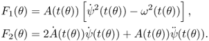
The dominant terms in the forcing for p are the forcing terms F1 and F2 as Ä is small as ω is assumed to be slowly varying. Equation 3.15 with the forcing terms F1 and F2 can be solved using variation of parameters as
3.17 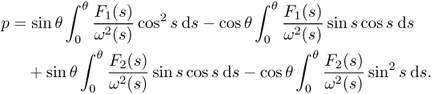
For this to be a valid approximate solution, we need p(θ) to remain bounded as θ increases. To study the behavior of p, let us study the first term in this solution, written as
3.18 
after an integration by parts. The second and third terms on the right-hand side are bounded functions of θ, leading to an acceptable solution for p(θ). However, the first term grows proportional to θ, unless F1 = 0. This requirement gives Equation 3.6 for the amplitude A. A similar argument shows that we require F2 = 0 for a bounded solution. The term proportional to Ä in Equation 3.15 is also resonant, but smaller, giving a contribution of O(Äθ). The correction ![]() in this equation is of
in this equation is of ![]() and is also growing but is again of higher order. This analysis gives an estimate of the validity of the approximation, which shows that it is valid to a range of θ inversely proportional to Ä, which is large since Ä is assumed small. This procedure can be carried to all orders, and it was shown to be convergent by Hale [4]. The modulated solutions can therefore be constructed, taking advantage of the difference between the timescale of the period of the oscillator and the scale of the variation of the parameters in the simple harmonic oscillator equation (Eq. 3.1), which is slow compared to the oscillation frequency.
and is also growing but is again of higher order. This analysis gives an estimate of the validity of the approximation, which shows that it is valid to a range of θ inversely proportional to Ä, which is large since Ä is assumed small. This procedure can be carried to all orders, and it was shown to be convergent by Hale [4]. The modulated solutions can therefore be constructed, taking advantage of the difference between the timescale of the period of the oscillator and the scale of the variation of the parameters in the simple harmonic oscillator equation (Eq. 3.1), which is slow compared to the oscillation frequency.
The results obtained here can be phrased in a “two timing” or “ multiple scales” form, which is usual in the applied mathematics literature [3], in the following manner. Let us again consider the dominant terms in Equation 3.15 for p
Now the function F1(θ) is slowly varying in θ and so can be considered to be independent of θ in a cycle 0 ≤ θ ≤ 2π, which is what was described earlier. Equation 3.19 then becomes
This assumption is known as the two timing assumption, which is to treat the slow time t and the fast variable θ as independent variables. We require a periodic solution of Equation 3.20. The only way to obtain a periodic solution of this boundary value problem with periodic boundary conditions is to require the forcing term to be orthogonal to the corresponding null space. This condition gives the same result as the one obtained earlier through variation of parameters, as we obtain
3.21 ![]()
Hence, F1 = F2 = 0, as before. The separation of scales then provides a way of constructing approximate solutions.
A fundamental formulation by Whitham [1, 2] is based on the variational form of the equation to be solved. Let us revisit this alternative formulation. The simple harmonic oscillator equation (Eq. 3.1) is derived from the Lagrangian
Whitham's idea was to use a Galerkin approximation, but with a trial function in the form of a modulated oscillation. In this case, this trial function is
3.23 ![]()
so that
3.24 
and neglect, as before, terms involving ![]() . Substituting these expressions into the Lagrangian, Equation 3.22 gives
. Substituting these expressions into the Lagrangian, Equation 3.22 gives
Let us change the variable of integration to θ in the second integral, to give
3.26 
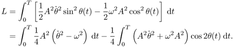
In the second integral on the right-hand side, the function t(θ) is slowly varying and is assumed to be constant in a cycle, which is equivalent to saying that t is independent of θ. The cos2θ term then integrates to 0, and the Lagrangian (Eq. 3.25) becomes
The modulation equations obtained by taking variations of the Lagrangian (Eq. 3.27) are again (Eq. 3.7) in the form ![]() , which is obtained by varying with respect to A, and
, which is obtained by varying with respect to A, and ![]() , which is obtained by varying with respect to θ. The modulation equations are then the variational equations of the averaged Lagrangian. The procedure outlined here can be phrased as saying that the modulation equations are obtained from the averaged Lagrangian
, which is obtained by varying with respect to θ. The modulation equations are then the variational equations of the averaged Lagrangian. The procedure outlined here can be phrased as saying that the modulation equations are obtained from the averaged Lagrangian
3.28 ![]()
where the variable θ is assumed to be independent of t, as before.
This method can be further developed to show how the orthogonality idea leads to the averaged Lagrangian formulation in general [1, 2]. Indeed, the method can be extended to dispersive wave equations, leading to clearly interpretable modulation equations for the slowly varying wave parameters [1, 2]. In the next section, we show how suitable trial functions with prescribed spatial profiles modulated in the evolution variable with slowly varying parameters can be used effectively to describe the evolution of coherent structures of interest. Moreover, we show how the modulation theory for coherent structures can be coupled with the radiation emitted as they evolve.
3.2 Survey of Perturbation Methods for Solitary Waves
Many nonlinear dispersive wave equations describing physical processes have solitary wave solutions, standard examples with applicability to a wide range of physical systems being the Korteweg-de Vries (KdV) equation, the nonlinear Schrödinger (NLS) equation, and the Sine–Gordon equation [1, 5]. In standard form, these equations are derived for nonlinear wave propagation in uniform media. In most applications, however, the propagation medium is rarely uniform. In the case in which the medium is slowly varying, so that the length scale for the variation of the medium is much greater than a characteristic length of the nonlinear wave—for instance, the width of a solitary wave or the wavelength of a periodic wave—perturbation methods can be employed to determine the changes in the properties of the wave as it propagates through the changing medium, much as for the simple harmonic oscillator example of the previous section [3]. As the medium is slowly varying, the method of multiple scales [3] is usually employed. The actual method of multiple scales can be cast in many forms and is also called the method of averaging [3] and modulation theory [1]. It should be noted that the standard equations mentioned earlier, the KdV, NLS, and Sine–Gordon equations, are also standard examples of completely integrable equations that can be solved using the method of inverse scattering [6, 7]. In the special case in which an inverse scattering solution is available, soliton evolution in slowly varying media can be studied using perturbed inverse scattering theory [8]. However, as the emphasis of this chapter is nonlinear beam evolution in nematic liquid crystals, for which the governing equations do not have an inverse scattering solution, the method of perturbed inverse scattering is not discussed here.
To motivate the extension of modulation theory, which forms the core of the methods used to analyze the evolution of nonlinear beams in nematic liquid crystals, let us start with a simple problem of soliton evolution in a medium with slowly varying linear dispersion, governed by an NLS equation with slowly varying coefficients
Here, β is the linear diffraction and is a function of Z = ϵz, ϵ ![]() 1, ϵ > 0. The evolution of a solitary wave will be analyzed using three variations of the method of multiple scales, the standard form of multiple scales, the method of averaging and modulation theory. For constant β, the NLS Equation 3.29 has the soliton solution
1, ϵ > 0. The evolution of a solitary wave will be analyzed using three variations of the method of multiple scales, the standard form of multiple scales, the method of averaging and modulation theory. For constant β, the NLS Equation 3.29 has the soliton solution
Let us first use the standard method of multiple scales to analyze the evolution of the soliton (Eq. 3.30) for slowly varying β [3]. We therefore seek a perturbation series solution of the form
We now substitute the perturbation series (Eq. 3.31) into the NLS equation (Eq. 3.29) and separate terms in powers of ϵ. At O(1), we obtain the soliton solution (Eq. 3.30) with σ′ = a2/2. At O(ϵ), we obtain
where the asterisk superscript denotes the complex conjugate and
3.33 ![]()
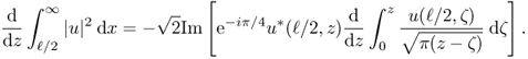
To eliminate secular terms, that is, terms that grow in x, from the solution of Equation 3.32 for u1, the right-hand side of this equation must be orthogonal to the bounded solutions of the adjoint of P(u1) [3]. There are two bounded solutions of the adjoint, u0x and u0z. The right-hand side of Equation 3.32 must then be orthogonal to ![]() and sech φ. As the right-hand side is even in x, it is automatically orthogonal to the first of these. Enforcing orthogonality to the second solution, that is, the integral from x = − ∞ to x = ∞ of the right-hand side times sech φ is zero, gives the differential equation for the amplitude a of the soliton
and sech φ. As the right-hand side is even in x, it is automatically orthogonal to the first of these. Enforcing orthogonality to the second solution, that is, the integral from x = − ∞ to x = ∞ of the right-hand side times sech φ is zero, gives the differential equation for the amplitude a of the soliton
which has the solution
with a(0) and β(0) being a and β at z = 0. This equation gives the evolution of the amplitude of the soliton as it propagates through the medium with slowly varying linear diffraction.
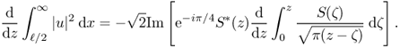
Let us now analyze the evolution of the soliton using the method of averaging [3]. Multiplying the NLS equation (Eq. 3.29) by u* and subtracting the complex conjugate of the resulting equation gives, after some manipulation,
This equation is formally termed conservation of mass, as it corresponds to invariance in phase of the Lagrangian for the NLS equation (Eq. 3.29) [8]. Whereas it physically corresponds to conservation of mass in the application of the NLS equation to water waves, in the optical context, it corresponds to conservation of power [5]. Integrating this mass conservation in x from − ∞ to ∞, which is termed as averaging in x, gives
3.37 ![]()
Substituting the soliton solution (Eq. 3.30) into this integral gives the differential equation for the amplitude
3.38 ![]()
This is the same differential equation (Eq. 3.34) as that obtained using a multiple scales analysis, and so has the same solution (Eq. 3.35). It is readily apparent that the use of averaging has resulted in a much more rapid and simple derivation of the equation governing the evolution of the soliton than the multiple scales analysis. Its simplicity is its key attraction. In fact, the orthogonality condition resulting from the multiple scales analysis is nothing more than the conservation of mass relation in integral form for the basic solution u0. A word of caution needs to be noted, though. As the NLS equation has an inverse scattering solution, it has an infinite number of conservation laws [1, 6, 7]. The question then arises as to why the conservation of mass equation, the lowest order conservation equation, was used to derive the equation for the evolution of the amplitude of the soliton. The use of this equation, of course, agrees with the formal multiple scales analysis. In general, the orthogonality relation from a multiple scales analysis corresponds to the lowest order conservation law(s). The use of the correct conservation laws for an averaging analysis of a slowly varying equation can be quite subtle. In the case of the KdV equation, the use of the lowest order conservation law, that of mass, does not lead to the correct equation for the evolution of a slowly varying KdV soliton [9]. This is because as the soliton evolves, it sheds an O(1) amount of mass, which must be included in the mass conservation law [9]. The correct conservation law to use in this case is that of energy, also called momentum. This is because the shed radiation has an O(ϵ) amount of energy. A full multiple scales analysis will lead to the correct orthogonality relation being the energy conservation (momentum conservation) integral. A slowly varying NLS soliton does not shed an O(1) amount of mass, so mass conservation gives the correct orthogonality relation. The topic of the radiation shed by slowly varying solitons is taken up later in this chapter.
Modulation theory was originally developed by Whitham [1, 2] to analyze slowly varying nonlinear, dispersive wave trains. This method is based on averaging a Lagrangian for the governing equation, in the same sense as the method of averaging averages conservation laws. The two averaging techniques are related, as by Nöther's Theorem conservation equations arise from invariances of the Lagrangian [10]. Although the modulation theory was originally developed for periodic wave trains, it can still be used for solitary waves as a solitary wave is a limiting case of a periodic wave for which the period goes to infinity, within which limit an isolated wave is obtained. The Lagrangian for the NLS equation (Eq. 3.29) is
The key to modulation theory is to take the exact soliton, or periodic wave, solution and assume that its parameters are slowly varying functions. If the soliton u0 in Equation 3.31 is now substituted into this Lagrangian and the Lagrangian averaged by integrating in x from − ∞ to ∞, the averaged Lagrangian
3.40 ![]()
results, where the derivative is with respect to Z = ϵz. Taking variations of this averaged Lagrangian with respect to a and σ gives
3.41 ![]()
3.42 ![]()
These two equations lead to the same results as the multiple scales and averaging analyses.
The averaged Lagrangian method can be extended by letting the slowly varying soliton have an arbitrary width and then letting the modulation equations determine the amplitude/width relation. We then set
3.43 ![]()
where, as before, a, w, and σ are functions of Z. Substituting this solution form into the Lagrangian (Eq. 3.39) and averaging in x results in the averaged Lagrangian
3.44 ![]()
Taking variations with respect to the soliton parameters then results in the modulation equations
3.45 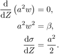
These modulation equations lead to the same results as before. The appropriate use of the variational principle and the averaged Lagrangian will then lead to the correct soliton relations [1].
3.3 Linearized Perturbation Theory for Nonlinear Schrödinger Equation
Before proceeding to develop modulation theory for the evolution of a soliton from an initial condition for the NLS equation, let us consider soliton perturbation theory. The results of this theory will be compared and contrasted with the results of modulation theory in Section 3.4.
A standard approach used to study small perturbations for a soliton is to use perturbation theory based on linearizing about the exact soliton solution [11, 12]. This leads to the study of an initial value problem for a linear equation, which can be solved using an appropriate eigenfunction expansion. This eigenfunction expansion includes both the localized, discrete spectrum and the corresponding projections on the continuous spectrum. It is the spectrum of the linearized equation that determines the behavior of the solution. This equation then needs to be analyzed in detail. Let us now assume that the linear diffraction is constant and set β = 1 in the NLS equation (Eq. 3.29)
This equation has the one parameter family of soliton solutions
To study the linearized stability of the soliton u0, let us take the perturbation expansion u = u0 + v, where |v| ![]() |u0|. The equation for v is then
|u0|. The equation for v is then
3.48 ![]()
with v(x, 0) = f(x) a given initial condition. This equation can be solved using Laplace transforms. The inversion of this Laplace transform solution is calculated in terms of singularities, which are poles corresponding to the eigenfunctions of the operator P defined by
and branch points that give the contribution of the continuous spectrum. It should be noted that the operator P is not self-adjoint, so that the poles can be double poles, giving Jordan blocks [13]. These double poles always lead to linear growth in z of the solution for v, just as for the linear resonance discussed in Section 3.2 when the perturbation solution of Equation 3.29 was developed. These resonant terms were eliminated by modulating the soliton parameters to eliminate this growth. It is clear from the definition (Eq. 3.49) that as |x| → ∞, Pv → vxx/2 and that P has a real continuous spectrum λ = − k2, which gives the radiation modes.
The detailed analysis of the point spectrum of P is given in Reference 14. It was shown that the corresponding eigenspace gives a Jordan block of dimension 4. This eigenspace is spanned by the eigenfunctions φ1(x) = sech ax and ![]() , which satisfy the eigenvalue equation Pφ1 = 0 and Pφ2 = 0, and the functions
, which satisfy the eigenvalue equation Pφ1 = 0 and Pφ2 = 0, and the functions ![]() and φ4(x) = xsech ax, which satisfy Pφ3 = φ1 and Pφ4 = φ2. We again note that Equation 3.34 for the slowly varying parameters of the slowly varying soliton (3.31) was obtained by requiring orthogonality of φ1 and φ2 to the right-hand side of the first-order perturbation equation (Eq. 3.32). We note that the solution for v takes the form
and φ4(x) = xsech ax, which satisfy Pφ3 = φ1 and Pφ4 = φ2. We again note that Equation 3.34 for the slowly varying parameters of the slowly varying soliton (3.31) was obtained by requiring orthogonality of φ1 and φ2 to the right-hand side of the first-order perturbation equation (Eq. 3.32). We note that the solution for v takes the form
The coefficients A1, A2, A3, and A4 and the function A(k) are determined from the initial condition. This solution can be interpreted as follows. The contributions of φ1 and φ2 account for a shift in the phase and a position shift, respectively, as can be seen by expanding the soliton solution (Eq. 3.47) in a Taylor series with respect to x0 and a. The function φ4 accounts for the soliton's acceleration, whereas φ3 accounts for the distortions in the soliton's width.
The continuous contribution has the form of a shelf as k → 0, because it takes the form
3.51 ![]()
for x ∼ 0. This is a shelf that oscillates with frequency 2σ. We thus see that this shelf can be approximated in the form A(0)exp(2iσz) for − 1/a ≤ x ≤ 1/a. This suggests a trial function for the varying soliton of the form
where g(z) = 0 for |x| ≥ ![]() and
and ![]() is the length of the shelf. To agree with the solution (Eq. 3.50) for v, we can take
is the length of the shelf. To agree with the solution (Eq. 3.50) for v, we can take ![]() = w. The leading order trial function for the varying soliton then includes a contribution of the continuous spectrum, which is given by the shelf g. If the shelf length
= w. The leading order trial function for the varying soliton then includes a contribution of the continuous spectrum, which is given by the shelf g. If the shelf length ![]() is left as a free parameter in an averaged Lagrangian, we observe that the resulting modulation equations have a fixed point when a = 1/w, g = 0, and
is left as a free parameter in an averaged Lagrangian, we observe that the resulting modulation equations have a fixed point when a = 1/w, g = 0, and ![]() , which is the exact soliton solution. This trial function and modulation theory are taken up further in Section 3.4.
, which is the exact soliton solution. This trial function and modulation theory are taken up further in Section 3.4.
The solution (Eq. 3.52) must be consistent with the solution (Eq. 3.50) of the linearized equation. As the soliton fixed point is a center, its frequency must be ![]() . This requirement will give the length
. This requirement will give the length ![]() of the shelf discussed in the previous paragraph. It should be noted that the shelf arising from the continuous spectrum has the largest overlap with the eigenfunction φ3, which controls the evolution of the soliton's width. This shows the strong interaction between the width and the continuous spectrum, which in turn shows that w and g are conjugate variables in the sense of classical mechanics, as are a and
of the shelf discussed in the previous paragraph. It should be noted that the shelf arising from the continuous spectrum has the largest overlap with the eigenfunction φ3, which controls the evolution of the soliton's width. This shows the strong interaction between the width and the continuous spectrum, which in turn shows that w and g are conjugate variables in the sense of classical mechanics, as are a and ![]() .
.
Finally, using a more conventional perturbation theory approach, it was shown that the nonlinear terms of the NLS equation give the excitation of the radiation due to the appropriate resonance and projection onto the continuous spectrum [14]. The main contribution is from φ1, which shows that it is a mass imbalance that triggers the shedding of diffractive radiation. In the variational formulation of Section 3.4, this projection is replaced by the boundary condition of the solution of a linear equation that accounts for the imbalance in mass between the exact soliton solution and the modulated one.
3.4 Modulation Theory: Nonlinear Schrödinger Equation
All three techniques used in Section 3.2 to analyze slowly varying waves are based on allowing the exact soliton solution to have slowly varying parameters. Many equations governing nonlinear waves in physical applications do not possess exact periodic or solitary wave solutions, particularly in more than one space dimension. An example of relevance here is nonlinear beam evolution in nematic liquid crystals [15–17]. The question naturally arises as to how to perform any analysis of nonlinear wave evolution in such cases, other than by obtaining full numerical solutions of the governing equations. One approach that is successful in such cases is the “chirp” variational approach developed by Anderson [18]. This approach also solved another problem that arises for soliton evolution. Any initial condition for the NLS equation will evolve into a finite number of solitons, plus diffractive radiation, as long as the mass of the initial condition is above a critical value [6, 7]. The question then arises as to how to analyze this evolution from an initial condition to solitons, in the simplest case for which only one soliton is formed. For the production of a single soliton, the simplest case is a sech initial condition as then the initial condition can be envisaged as “slowly varying” from initial to final steady soliton state.
The standard NLS equation (Eq. 3.46) with constant linear diffraction has the Lagrangian
We shall take an initial condition of the form
3.54 ![]()
An obvious assumption is to seek a varying soliton-like solution of the form
where the amplitude a, width w, and phase σ are functions of z. Substituting this trial function into the Lagrangian (Eq. 3.53) and averaging in x yields the averaged Lagrangian
3.56 ![]()
Variations of this averaged Lagrangian, and some manipulation gives the variational, or modulation, equations
3.57 ![]()
3.58 ![]()
3.59 ![]()
It is readily apparent that a and w are then constants and the initial condition does not evolve. The trial function (3.55) is then an inadequate approximation to allow the initial condition to evolve to a soliton. Anderson overcame this problem by adding “chirp” to the trial function (Eq. 3.55)
The addition of this phase contribution was motivated by solutions of the linearized NLS (Schrödinger's) equation (Eq. 3.46). With the addition of this chirp, the resulting modulation equations allowed the initial condition to evolve. The chirp method is not continued further here for one vital reason. The modulation equations arising from the chirp trial function form a nonlinear oscillator and the amplitude and width do not evolve to a steady state but oscillate about a mean [19].
Inverse scattering theory shows that an initial condition evolves in a soliton(s) via the shedding of diffractive radiation [6, 7]. The trial function (Eq. 3.60) does not include this radiation loss and so cannot give modulation equations whose solution evolves to a steady state. To date, there has been no extension of the chirp method that includes this shed radiation. A successful method based on the extension of trial functions of the form (Eq. 3.55) and one that includes radiation loss was developed by Kath and Smyth [19]. The trial function used for the NLS equation was
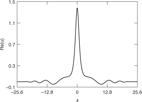
where the parameters a, w, σ, and g are functions of z. The first term is a varying soliton, as discussed earlier. The origin and importance of the second term is less clear. In Section 3.3, we showed how this shelf term arises out of linearized soliton perturbation theory. It can also be shown to arise from perturbed inverse scattering theory, which is taken up later. Before we consider this, it is noted that the physical effect of this shelf term is that it represents the effect of the low wave number radiation that accumulates under the soliton as it evolves. The linearized NLS equation (Eq. 3.46) (in fact Schrödinger's equation) has the dispersion relation ω = k2/2, so that the group velocity is cg = k. Hence, shed low wave number diffractive waves have low group velocity and so accumulate under the soliton as it evolves, forming a shelf of radiation. This shelf of radiation under a pulse is well known in the context of pulse propagation in optical fibers and is referred to as a pedestal [20, 21]. Figure 3.1 shows a numerical solution of the NLS equation (Eq. 3.46) for a nonsoliton initial condition and the shelf of radiation under the pulse can be clearly seen.
Figure 3.1 Numerical solution of NLS equation (Eq. 3.46) for initial condition u(x, 0) = 1.25 sech x. Source: Reproduced with permission from Fig. 2 in Reference 19.
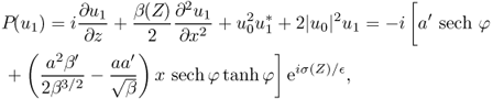
The existence of the shelf of radiation under an evolving soliton can also be demonstrated through a perturbation analysis based on the inverse scattering solution for the NLS equation. Let us linearize about an exact soliton
3.62 ![]()
with u = u0 + u1, where |u1| ![]() |u0|. Substituting this expansion into the NLS equation (Eq. 3.46) gives
|u0|. Substituting this expansion into the NLS equation (Eq. 3.46) gives
3.63 ![]()
where the phase θ = a2z/2 and f is the solution of
with the initial condition for f depending on u0(x, 0) [22]. Owing to diffraction, solutions of Equation 3.64 rapidly become flat as z → ∞. Therefore, for large z
3.65 ![]()
with h = − a2f. Hence, for large z
where ![]() . This approximation for large z closely resembles the trial function (Eq. 3.61), with the first term the varying soliton and the third term the flat shelf π/2 out of phase with the soliton. The question then is, what does the second term represent? This can be seen on expanding a sech x/w around an exact soliton. For an exact soliton, the width–amplitude relation is wf = 1/af. Hence, perturbing from an exact soliton with w = 1/af + δw and a = af + δa gives
. This approximation for large z closely resembles the trial function (Eq. 3.61), with the first term the varying soliton and the third term the flat shelf π/2 out of phase with the soliton. The question then is, what does the second term represent? This can be seen on expanding a sech x/w around an exact soliton. For an exact soliton, the width–amplitude relation is wf = 1/af. Hence, perturbing from an exact soliton with w = 1/af + δw and a = af + δa gives
3.67 ![]()
Around x = 0 the perturbing term from the exact soliton is δa. Similarly near x = 0 the second term in Equation 3.66 is − |h|cosψ. The second term in (3.66) then represents changes in the amplitude of the soliton as it evolves. Finally, it should be noted that the soliton perturbation theory leading to (3.66) has aw = 1, so that δw = − δa/a2 within this theory. This analysis shows that the second term in Equation 3.66 is incorporated in the trial function (Eq. 3.61) through changes in a and does not need to be separately incorporated, unlike the shelf term, the third term in Equation 3.66. The shelf term adds in and out of phase with the soliton, causing the soliton to oscillate in amplitude as it evolves. Furthermore, the shelf term is π/2 out of phase with the soliton as the in-phase corrections are accounted for by variations in the amplitude and width of the soliton. The existence of a shelf of low wave number radiation under evolving solitons has also been shown for coupled NLS equations [11, 12].
The shelf of radiation under the evolving soliton, determined by g, must have limited extent and must match the radiation propagating away from the evolving soliton, as seen in Figure 3.1. It is then assumed that the shelf has length ![]() , so that it extends in the region −
, so that it extends in the region − ![]() /2 ≤ x ≤
/2 ≤ x ≤ ![]() /2, as previously discussed in Section 3.3. The length
/2, as previously discussed in Section 3.3. The length ![]() is determined from the modulation equations given later.
is determined from the modulation equations given later.
Substituting the trial function into the Lagrangian (Eq. 3.53) and averaging in x results in the averaged Lagrangian
3.68 ![]()
Taking variations of this averaged Lagrangian gives the modulation equations
These modulation equations have the fixed point afwf = 1 and g = 0, which is the soliton solution of the NLS equation, as required.
Using Nöther's Theorem on the NLS Lagrangian (Eq. 3.53) [10], the NLS equation (Eq. 3.46) has the energy conservation equation
3.73 ![]()
Averaging this energy conservation equation gives the modulation equation for conservation of energy
As at the soliton steady state afwf = 1, this energy conservation equation gives this steady state given the initial values of a and w, a(0) and w(0),
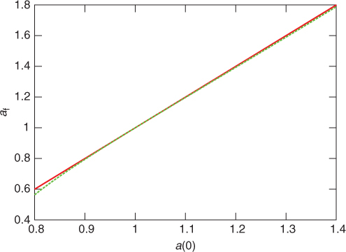
Inverse scattering gives that for an initial width w(0) = 1, the amplitude of the final soliton is [23]
Figure 3.2 shows a comparison between the final soliton amplitudes as given by inverse scattering and modulation theory. It can be seen that modulation theory is in excellent agreement with the inverse scattering result. It should be noted that the inverse scattering result is valid for a(0) > 1/2. Below this initial amplitude, no soliton is formed as, unlike for the KdV equation, the NLS equation requires a critical initial mass for a soliton to form [6, 7].
Figure 3.2 Comparison of final soliton amplitude af for initial condition a(0) sech x. Inverse scattering (Eq. 3.76): solid line; modulation theory (Eq. 3.75): dashed line.
The Lagrangian (Eq. 3.53) also has scale invariance. Applying Nöther's Theorem [10] to this scale invariance leads to the mass conservation equation
This is the same as the mass conservation equation (Eq. 3.36) for constant linear diffraction, as expected. Averaging this mass conservation equation using the trial function (3.61) gives the modulation equation (Eq. 3.69).
The final quantity to be determined is the length ![]() of the shelf of radiation under the evolving soliton. Let us linearize the modulation Equations 3.69–3.72 about the steady state with a = af + a1, w = 1/af + w1, and g = g1, |a1|
of the shelf of radiation under the evolving soliton. Let us linearize the modulation Equations 3.69–3.72 about the steady state with a = af + a1, w = 1/af + w1, and g = g1, |a1| ![]() af, |w1|
af, |w1| ![]() wf, and |g1|
wf, and |g1| ![]() 1. After some algebra, we find w1 = − 2a1/af with g1 satisfying the simple harmonic oscillator equation
1. After some algebra, we find w1 = − 2a1/af with g1 satisfying the simple harmonic oscillator equation
3.78 ![]()
As discussed in Section 3.3, near the steady state, the shelf oscillates with the soliton frequency
![]() [19]. Hence, we find the shelf length
[19]. Hence, we find the shelf length
3.79 ![]()
3.5 Radiation Loss
The modulation equations (Eqs. 3.69, 3.70, 3.71, 3.72) of the previous section cannot evolve to a steady state as they form a conservative system. Their solution will oscillate about a mean indefinitely. General initial conditions for solitary wave equations evolve to solitary wave steady states through shedding diffractive radiation [1, 6, 7]. This diffractive radiation is the physical and mathematical effect missing from the modulation equations of Section 3.4. Figure 3.1 shows that the shed radiation has small amplitude relative to the evolving solitary wave. The NLS equation (Eq. 3.46) then shows that it is governed by the linearized NLS (Schrödinger's) equation
subject to a boundary condition that matches the shed radiation to the edge of the shelf, u = S(z) at x = ± ![]() /2. As there is no radiation initially, this equation is solved together with the initial condition u = 0 at z = 0. There are a number of ways to solve Equation 3.80, but the easiest is to use Laplace transforms in z.
/2. As there is no radiation initially, this equation is solved together with the initial condition u = 0 at z = 0. There are a number of ways to solve Equation 3.80, but the easiest is to use Laplace transforms in z.
The key quantity to determine to account for the effect of the shed diffractive radiation in the modulation equations is the mass flux associated with this shed radiation. This radiation also takes away energy from the soliton, but this loss is second order [19]. Integrating the mass conservation equation (Eq. 3.77) from the edge of the shelf at x = ![]() /2 to ∞ gives the mass loss flux to x >
/2 to ∞ gives the mass loss flux to x > ![]() /2 as
/2 as
By symmetry, there is an identical mass flux into x < − ![]() /2. To determine the amount of mass lost by the soliton as it evolves, we then need to determine u and ux at the edge of the shelf x =
/2. To determine the amount of mass lost by the soliton as it evolves, we then need to determine u and ux at the edge of the shelf x = ![]() /2.
/2.
Assigning s as the Laplace transform variable and denoting transforms by a ![]() superscript, we find Equation 3.80 becomes
superscript, we find Equation 3.80 becomes
3.82 ![]()
Taking the solution of this equation that decays at ∞ by taking the correct branch for the square root of − i, we have
3.83 ![]()
where A is a constant of integration. Hence,
3.84 ![]()
Inverting this Laplace transform using the convolution theorem gives
3.85 ![]()
We then see that all we need to determine the mass flux to the diffractive radiation in x > ![]() /2 is u(
/2 is u(![]() /2, z). From Equation 3.81, this mass flux to x >
/2, z). From Equation 3.81, this mass flux to x > ![]() /2 is
/2 is
To complete the radiation analysis, we need to determine the function S(z). In the vicinity of the shelf, the trial function 3.61 can be decomposed into the fixed-point soliton, plus a component that must radiate away, so that
3.87 ![]()
where u1 is the radiated component. From Figure 3.1, it can be seen that |u1| is small relative to |ufixed|. The mass in the combined soliton and shelf is then
3.88 ![]()
If we assume a small overlap between ufixed and u1, we have from the mass equation (Eq. 3.69) that
3.89 ![]()
near the fixed point, due to symmetry, where the f subscripts denote fixed-point values. Mass conservation then gives
as afwf = 1 and S = u1 at x = ± ![]() /2. Using this value of u at the edges of the shelf in the mass flux equation (Eq. 3.86), we have
/2. Using this value of u at the edges of the shelf in the mass flux equation (Eq. 3.86), we have
The shelf of radiation under the soliton is flat, so that its phase will be slowly varying. The phase of S will then be slowly varying. If we set S in polar form as S = Rexp(iφ), we can approximate the mass flux (Eq. 3.91) by
3.92 
with R = |S| determined by Equation 3.90. The mass flux to the left of the soliton will also be given by this expression by symmetry.
Adding the mass flux expression to the mass modulation equation (Eq. 3.69), we obtain
where the loss coefficient δ is
3.94 ![]()
with
3.95 ![]()
To add the mass loss in a consistent manner to the modulation Equations (3.69, 3.70, 3.71, 3.72), we need to leave the energy Equation 3.74 unchanged as the energy lost in the diffractive radiation is second order [19]. To achieve this, we need to add a loss term to the g equation (Eq. 3.71) [19], so that this equation becomes
The final set of modulation equations governing the evolution of the soliton is then Equations 3.70, 3.72, 3.93, and 3.96. The mass equation (Eq. 3.93) can be replaced by the energy equation (Eq. 3.74), as was done by Kath and Smyth [19], as it is not independent of the modulation Equations (3.69, 3.70, 3.71, 3.72).
Figure 3.3 shows a comparison between the soliton amplitude as given by the full numerical solution of the NLS equation (Eq. 3.46) and the modulation equations with mass loss to shed diffractive radiation. It can be seen that there is an excellent comparison. The numerical amplitude decays to the steady state at a slightly faster rate than the modulation amplitude. Because the modulation equations form a nonlinear damped oscillator, the difference in decay rate translates into a difference in the period of the oscillation, as seen in the figure. Finally, the mean of the modulation oscillation is slightly lower than that of the numerical solution, which means that the steady state of the numerical solution is slightly higher than that of the modulation solution.
Figure 3.3 Comparison of amplitude a of soliton as given by the full numerical solution of the NLS equation (Eq. 3.46) (solid line) and the modulation equations (dashed line) for the initial condition a = 1.25 and w = 1. Source: Reproduced with permission from Fig. 4 in Reference [19].
3.6 Solitary Waves in Nematic Liquid Crystals: Nematicons
The ideas and techniques developed in the previous section for the NLS equation can be applied to analyze the motion of solitary wave beams in a nematic liquid crystal, so-called nematicons [15]. These nonlinear beams are two space dimensional, which makes the analysis more complicated than that of the one space dimensional NLS equation. At the simplest level, nematicons can be taken to be circularly symmetric, even though they have slight ellipticity [24].
Let us consider the propagation of a polarized, coherent light beam (laser light) through a cell filled with a nematic liquid crystal. The direction down the cell is the z-direction and the (x, y) plane is orthogonal to this. The beam is polarized in the x-direction and an external static electric field is applied in the x-direction to pretilt the nematic molecules at an angle θ0 to the z-direction. This external field helps overcome the Freédericksz threshold for the nematic so that a low power light beam can self-focus as the total electric field—external plus the electric field of the electromagnetic radiation—is above the threshold. The perturbation of the director angle from the pretilt is denoted by θ. The envelope of the electric field of the light is denoted by ![]() . Typical dimensions are ∼ 100 μm for the cell width, ∼ 1 mm for the cell length, and ∼ 5 μm for the beam width [24]. Owing to the small size of the beam relative to the cell, if the beam is launched near the center of the cell, the effect of the cell boundaries on its propagation can be ignored. In nondimensional form, the equations governing the propagation of the beam are [16, 17, 25]
. Typical dimensions are ∼ 100 μm for the cell width, ∼ 1 mm for the cell length, and ∼ 5 μm for the beam width [24]. Owing to the small size of the beam relative to the cell, if the beam is launched near the center of the cell, the effect of the cell boundaries on its propagation can be ignored. In nondimensional form, the equations governing the propagation of the beam are [16, 17, 25]
3.98 ![]()
Here, the Laplacian ∇2 is in the (x, y) plane. In mathematical terms, the distance z down the liquid crystal cell is a timelike variable for the NLS-type equation (Eq. 3.97). The parameter ν is related to the elastic properties of the liquid crystal and, in most experimental situations, is large, typically O(100) [15, 16]. The limit of large ν is called the nonlocal limit. The parameter q is related to the square of the external pretilting electric field [16, 17, 26]. Finally, the parameter Δ is the birefringent walk-off of the Poynting vector [1, 25].
If the medium is uniform, the walk-off term in the electric field equation (Eq. 3.97) can be factored out by the phase transformation [27]
The nematicon Equations 3.97 and 3.98 then become
The transformation (Eq. 3.99) is, of course, only valid if the liquid crystal is in a uniform state. In Chapters 1, 5, and 11, examples will be considered for which this walk-off term needs to be retained as nonuniformities in the medium due, for example, to a varying static pretilting field or the influence of other light beams, mean that the walk-off varies across the liquid crystal cell, altering the nematicon trajectory. As the nonlocality parameter ν increases, the perturbation θ of the director from the pretilt θ0 decreases as ![]() [28, 29]. In experimental situations, ν is usually in the range O(10)–O(100) [16, 24, 26]. So for the milliWatt beam powers employed in experiments, the angle θ is small and the trigonometric functions in the full nematicon equations (Eqs. 3.100, 3.101) can be approximated by the first terms in their Taylor series, giving the simplified nematicon equations
[28, 29]. In experimental situations, ν is usually in the range O(10)–O(100) [16, 24, 26]. So for the milliWatt beam powers employed in experiments, the angle θ is small and the trigonometric functions in the full nematicon equations (Eqs. 3.100, 3.101) can be approximated by the first terms in their Taylor series, giving the simplified nematicon equations
These small deviation nematicon equations are amenable to analysis using the same variational techniques as for the NLS equation in Section 3.4. Numerical solutions have shown that the nematicon equations have a solitary wave solution, termed a nematicon [15–17]. However, to date, no exact nematicon solution has been found for either the full nematicon Equations 3.100 and 3.101 or the simplified Equations 3.102 and 3.103. As discussed previously, this means that standard perturbation techniques cannot be used to analyze nematicon evolution, leaving full numerical solutions and variational techniques the main avenues for such analysis. This section discusses the application of variational techniques to the nematicon Equations 3.102–3.103. For circularly symmetric solutions, the nematicon Equations 3.102 and 3.103 have the Lagrangian
In analogy with the trial function (Eq. 3.61) for the NLS equation, we shall develop modulation equations for nematicon evolution based on the trial functions
for the electric field and the optical axis, where ![]() [30]. The trial function for the electric field is the same as that for the NLS equation, but in radially symmetric form as the nematicon equations are in two space dimensions. The new trial function is that for the optical axis. In the nonlocal limit with ν large, the optical axis perturbation extends far beyond the waist of the electric field solitary wave [15–17]. Therefore, the optical axis has a different width from that of the electric field. The forcing in the Poisson Equation 3.103 for the director is proportional to |E|2. Hence, the functional form for the optical axis is assumed to be the square of that for the electric field. As for the NLS equation, the shelf of low wave number diffractive radiation under the beam must have limited extent before it matches the radiation propagating away from the beam. It is then assumed that g is nonzero in the disk 0 ≤ r ≤
[30]. The trial function for the electric field is the same as that for the NLS equation, but in radially symmetric form as the nematicon equations are in two space dimensions. The new trial function is that for the optical axis. In the nonlocal limit with ν large, the optical axis perturbation extends far beyond the waist of the electric field solitary wave [15–17]. Therefore, the optical axis has a different width from that of the electric field. The forcing in the Poisson Equation 3.103 for the director is proportional to |E|2. Hence, the functional form for the optical axis is assumed to be the square of that for the electric field. As for the NLS equation, the shelf of low wave number diffractive radiation under the beam must have limited extent before it matches the radiation propagating away from the beam. It is then assumed that g is nonzero in the disk 0 ≤ r ≤ ![]() .
.
Substituting the trial functions (Eq. 3.105) into the Lagrangian (Eq. 3.104) and averaging by integrating in r from 0 to ∞ gives the averaged Lagrangian [30]
Here, Λ = ![]() 2/2. The various integrals Ii and Ii, j in this averaged Lagrangian are listed in Appendix 3.A. There is one complication in the calculation of this averaged Lagrangian. Inspection of the Lagrangian (Eq. 3.104) shows that the integral
2/2. The various integrals Ii and Ii, j in this averaged Lagrangian are listed in Appendix 3.A. There is one complication in the calculation of this averaged Lagrangian. Inspection of the Lagrangian (Eq. 3.104) shows that the integral
needs to be evaluated. This integral can only be evaluated exactly for w = β, which is not the case in the nonlocal limit with β ![]() w. One option is to evaluate the integral (Eq. 3.107) numerically, which also means evaluating its derivatives with respect to w and β numerically too, as both of these will result when variations of the averaged Lagrangian are taken. However, an analytical approximation is possible. This relies on the idea of “equivalent functions” [30]. The sech functions in Equation 3.107 are replaced by Gaussians with adjustable width parameters, and these parameters are determined by requiring that the resulting integral matches with the exact integral (Eq. 3.107) in the nonlocal limit β
w. One option is to evaluate the integral (Eq. 3.107) numerically, which also means evaluating its derivatives with respect to w and β numerically too, as both of these will result when variations of the averaged Lagrangian are taken. However, an analytical approximation is possible. This relies on the idea of “equivalent functions” [30]. The sech functions in Equation 3.107 are replaced by Gaussians with adjustable width parameters, and these parameters are determined by requiring that the resulting integral matches with the exact integral (Eq. 3.107) in the nonlocal limit β ![]() w. The idea behind this substitution is that what is required in the averaged Lagrangian is an integral. If two different integrals have the same value, the averaged Lagrangian will be unchanged. So using the idea of “equivalent functions,” we replace sech2r/β by exp( − r2/(Aβ)2) and sech2r/w by exp( − r2/(Bw)2). Then,
w. The idea behind this substitution is that what is required in the averaged Lagrangian is an integral. If two different integrals have the same value, the averaged Lagrangian will be unchanged. So using the idea of “equivalent functions,” we replace sech2r/β by exp( − r2/(Aβ)2) and sech2r/w by exp( − r2/(Bw)2). Then,
Let us now evaluate the integral (Eq. 3.107) in the limit β ![]() w. Using the change of variable r = βρ and expanding in Taylor series for w/β
w. Using the change of variable r = βρ and expanding in Taylor series for w/β ![]() 1, this integral becomes
1, this integral becomes
where Ix32 is given in Appendix 3.A. Then expanding the equivalent integral (Eq. 3.108) in a Taylor series for w/β ![]() 1 and matching with Equation 3.109 gives the values of A and B listed in Appendix 3.A.
1 and matching with Equation 3.109 gives the values of A and B listed in Appendix 3.A.
Taking variations of the averaged Lagrangian (Eq. 3.106) with respect to the parameters a, w, α, β, σ, and g results in the variational equations
plus the algebraic equations
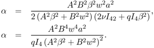
These modulation equations are the equations governing the evolution of the nematicon. The variational equation (Eq. 3.110) is the equation for conservation of mass in the sense of the invariance of the Lagrangian (Eq. 3.104) with respect to shifts in the phase [8]. In the present optical context, it is the equation for the conservation of optical power. Eliminating α between the algebraic equations (Eq. 3.114), the director angle width β can be found as
By Nöther's Theorem [10], the nematicon equations (Eqs. 3.102 and 3.103) have an energy conservation equation that can be obtained from the Lagrangian (Eq. 3.104) based on the invariance of the Lagrangian to shifts in z. This energy conservation equation is
3.116 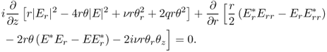
Averaging this energy conservation equation gives
As energy is conserved, this energy conservation equation can be used to determine the final steady nematicon state from the input beam.
The final parameter to be determined is the shelf radius ![]() . As in Section 3.4, this is determined by linearizing the modulation equations (Eqs. 3.110, 3.111, 3.112, 3.113, 3.114) about the fixed-point values af, wf, σf, αf, βf, and g = 0 to obtain a simple harmonic oscillator equation. The frequency of this oscillator is then equated to the nematicon frequency
. As in Section 3.4, this is determined by linearizing the modulation equations (Eqs. 3.110, 3.111, 3.112, 3.113, 3.114) about the fixed-point values af, wf, σf, αf, βf, and g = 0 to obtain a simple harmonic oscillator equation. The frequency of this oscillator is then equated to the nematicon frequency ![]() . In principle, the details are as for the NLS equation but are much more involved because of two trial functions being involved. The details are presented in Appendix 3.B.
. In principle, the details are as for the NLS equation but are much more involved because of two trial functions being involved. The details are presented in Appendix 3.B.
3.7 Radiation Loss for The Nematicon Equations
As a nematicon propagates down a cell, it sheds diffractive radiation so as to evolve to a steady state. The contribution of this radiation to the modulation equations of Section 3.6 can be calculated as for the NLS equation in Section 3.5. The major difference is that nematicons are circularly symmetric, so that the shed radiation will be expressed in terms of Bessel functions. Again, the shed radiation has small amplitude relative to the nematicon beam and so is governed by the linearized electric field equation (Eq. 3.102)
The solution of this linear equation must be matched with the electric field at the edge of the shelf, so that E = S(z) at r = ![]() . An identical argument as for the NLS equation in Section 3.5 yields
. An identical argument as for the NLS equation in Section 3.5 yields
3.119 ![]()
Again Nöther's Theorem gives the mass conservation equation for the radiation equation (Eq. 3.118) as
3.120 ![]()
Integrating this equation from the edge of the shelf to ∞ gives the mass flux to shed diffractive radiation as
To determine this mass flux, we again need to determine E and Er at the edge of the shelf. To use the mass flux expression, we will assume that the radius of the shelf ![]() is slowly varying relative to the time z scale for propagation of the shed radiation. Then,
is slowly varying relative to the time z scale for propagation of the shed radiation. Then, ![]() can be taken to be constant in the radiation calculation.
can be taken to be constant in the radiation calculation.
The radiation equation (Eq. 3.118) can again be solved using Laplace transforms and the convolution theorem used to relate Er to E at the edge of the shelf. The details will be omitted here as they are similar to those for the NLS equation in Section 3.5. Using the transforms listed in Reference 31, the final result is
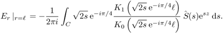
Here, K0 and K1 are the modified Bessel functions of orders 0 and 1, respectively, and C is the standard inversion contour for Laplace transforms. The loss flux on the right-hand side of Equation 3.121 is then
3.123 ![]()
where G is the Green's function
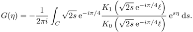
For simplicity, let us set S in polar form as S = R(z)exp(iφ(z)) and assume that the phase φ is slowly varying, as in Section 3.5. The mass flux can then be approximated as
The Green's function expression (Eq. 3.124), expressed in terms of an inverse Laplace transform, is too complicated as it stands to be of use in the modulation equations. The most useful approximation to make is to perform an asymptotic calculation of the flux for large z, which corresponds to s small in Laplace transforms [32]. To this end, the integrand in Equation 3.124, excluding exp(sη), can be rewritten as
3.126 ![]()
Now as z → 0, K0(z) ∼ − ln(z/2) [31]. Using this asymptotic value, the Green's function (Eq. 3.124) becomes
3.127 ![]()
This integral for the Green's function can now be evaluated by completing the contour around the branch point of the logarithmic function, adding the contributions from both sides of the branch cut and changing variables to -Re(s) = exp(ξ), to give
3.128 
This integral can now be evaluated for large η, which corresponds to large z in Equations 3.122 and 3.125, using the method of stationary phase. Adding this asymptotic value of the integral to the flux (Eq. 3.125) gives
Even though this integral contains the term 1/(z − z′), a careful examination of the integrand near z′ = z will show that the integral is convergent.
The mass flux in Equation 3.121 can now be evaluated by taking the imaginary part of Equation 3.129. As for the NLS modulation equations in Section 3.5, the mass flux can then be added to the mass modulation equation (Eq. 3.110). Again, for consistency, the modulation equation (Eq. 3.112) must be modified so that the mass equations (Eqs. 3.110, 3.112 for g, and 3.111) are consistent with the energy equation (Eq. 3.117). In this manner, it is found that the mass equation (Eq. 3.110) becomes
and Equation 3.112 becomes
where the loss coefficient δ is
and
There is, however, one subtle difference between the radiative loss from a nematicon and that from an NLS soliton, which can be seen by examining the solutions of the nematicon equations (Eqs. 3.100 and 3.101) shown in Figure 3.4. It can be seen that the shelf under the electric field beam extends well beyond the beam waist, in contrast to the NLS shelf shown in Figure 3.1, and forms a truncated cone. This extension of the shelf is due to the nonlocal nature of the nematic response in that the optical axis response away from electric field beam is forcing a new low wave number radiative mode. This extra shelf of radiation does not affect the frequency of the nematicon and the shelf length ![]() as it is away from the electric field beam and is due to the optical axis. However, it does have the effect of forcing the start of the propagating radiation away from what may be termed an inner shelf at r =
as it is away from the electric field beam and is due to the optical axis. However, it does have the effect of forcing the start of the propagating radiation away from what may be termed an inner shelf at r = ![]() to the end of this new outer shelf. This extended shelf of radiation was also found for coupled systems of NLS equations [11]. These two components of the shelf were shown to be due to two distinct types of eigenfunctions of the continuous spectrum for the equations describing the perturbation.
to the end of this new outer shelf. This extended shelf of radiation was also found for coupled systems of NLS equations [11]. These two components of the shelf were shown to be due to two distinct types of eigenfunctions of the continuous spectrum for the equations describing the perturbation.
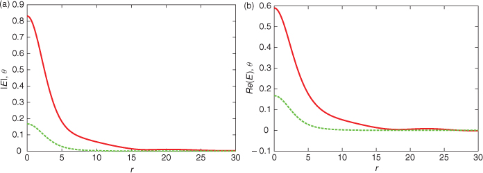
Figure 3.4 Numerical solution of nematicon equations (Eqs. 3.100 and 3.101) at z = 400 for the initial values a = 0.5 and w = 4. The parameter values are q = 2 and ν = 10. (a) Solution for |E|: solid line; solution for θ: dashed line, (b) solution for Re(E): solid line; solution for θ: dashed line.
Let us assume that the outer shelf has radius ρ. It was found from numerical solutions that this radius can be estimated as ρ = 7β1/2, where ![]() is the half-width of the optical axis [30]. In the loss terms in Equations 3.130, 3.131, 3.132, 3.133, the inner shelf area Λ =
is the half-width of the optical axis [30]. In the loss terms in Equations 3.130, 3.131, 3.132, 3.133, the inner shelf area Λ = ![]() 2/2 (modulo 2π) is replaced by the outer shelf area
2/2 (modulo 2π) is replaced by the outer shelf area ![]() (modulo 2π), so that the final modulation equations that incorporate mass loss to shed diffractive radiation are
(modulo 2π), so that the final modulation equations that incorporate mass loss to shed diffractive radiation are
and
where the loss coefficient δ is
3.136 
and
3.137 ![]()
The final set of modulation equations governing the evolution of the nematicon, which include loss to shed dispersive radiation, are Equations 3.111, 3.113, 3.114, 3.134, and 3.135.
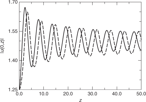
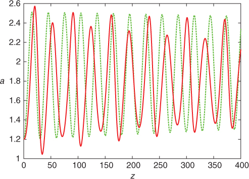
Figure 3.5 shows a comparison between the full numerical solution of the nematicon Equations 3.100 and 3.101 and the solution of the modulation equations. It can be seen that there is good agreement in the amplitude oscillations, with the mean of the modulation oscillation being the same as that of the numerical oscillation. This means that the modulation steady-state amplitude will be the same as that of the numerical solution. It can also be seen that the decay rate of the modulation solution is the same as that of the numerical solution, so that the radiation calculation of this section gives a good approximation to the flux of radiation from the evolving nematicon. There is a small difference in the periods of the amplitude oscillations. This is because the modulation period is determined by the shelf radius ![]() . The calculation of this radius carried out in the Appendix 3.B is based on linearizing the modulation equations about their fixed point. The evolution shown in Figure 3.5 is far from the steady state, so the difference in the two oscillation periods is not surprising. It can also be seen that there is a phase difference between the numerical and modulation amplitude oscillations. The phase is a higher order quantity in modulation theory and its calculation is, in general, nontrivial. The major difference between the numerical and modulation solutions is that the numerical solution shows a beating. The origin of this beating is that the numerical beam shape is undergoing significant changes during the evolution of the beam, as discussed further in Section 3.8. An important observation from Figure 3.5 is that the finite dimensional modulation theory does a very good job of capturing the dynamics of an infinite dimensional system.
. The calculation of this radius carried out in the Appendix 3.B is based on linearizing the modulation equations about their fixed point. The evolution shown in Figure 3.5 is far from the steady state, so the difference in the two oscillation periods is not surprising. It can also be seen that there is a phase difference between the numerical and modulation amplitude oscillations. The phase is a higher order quantity in modulation theory and its calculation is, in general, nontrivial. The major difference between the numerical and modulation solutions is that the numerical solution shows a beating. The origin of this beating is that the numerical beam shape is undergoing significant changes during the evolution of the beam, as discussed further in Section 3.8. An important observation from Figure 3.5 is that the finite dimensional modulation theory does a very good job of capturing the dynamics of an infinite dimensional system.
Figure 3.5 Comparison of amplitude a of nematicon as given by the full numerical solution of the nematicon equations (Eqs. 3.100 and 3.101) (solid line) and the modulation equations (dashed line). Initial conditions are a = 1.2, w = 3.5, with α and β determined by the first of Equations 3.114 and (3.115). The parameter values are q = 2 and ν = 100.
3.8 Choice of Trial Function
As there is no exact solitary wave, or nematicon, solution of the nematicon equations (Eqs. 3.102 and 3.103), the choice of trial function to model the evolution of a nematicon is much less clear than it was for the sech trial function (Eq. 3.61) for the NLS equation. Although a good agreement has been obtained for the evolution of a nematicon in the nonlocal limit with a sech trial function (Eq. 3.105), the exact nematicon profile is not of this form [16]. Near its peak, it has a Gaussian shape, and in its tails, it has the profile of the modified Bessel function K0 because of circular symmetry [16]. The choice of trial function then warrants further investigation.
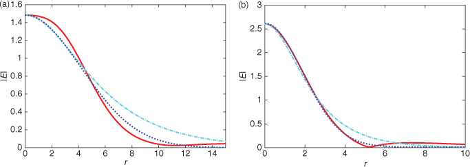
If the initial condition for the nematicon equations (Eqs. 3.100 and 3.101 or Eqs. 3.102 and 3.103) is not an exact nematicon solution, the beam evolves to an exact nematicon with its amplitude and width oscillating. Figure 3.6 shows the solution of the nematicon equations (Eqs. 3.100 and 3.101) for a sech initial condition with the same parameter values as the amplitude comparison of Figure 3.5. The solution is shown at a maximum of the amplitude oscillation and its neighboring minimum. To the numerical profile at these values of z, sech and Gaussian profiles have been fitted. It can be seen that at the minimum the beam shape is well presented by a sech, whereas at the maximum, the beam is better approximated by a Gaussian. It is known that in the extreme nonlocal limit, in essence ν infinite, that the steady nematicon profile is Gaussian [33], so the development of the beam shape in the nonlocal limit to a Gaussian during part of its oscillation is not surprising. However, the evolution of the beam is much more complicated than this comparison with the Gaussian of the extreme nonlocal limit, as shown in Figure 3.7, where similar comparisons are shown for a Gaussian initial condition for the same value of the nonlocality ν. Larger values of the initial amplitude and width have been chosen because of the faster decay of a Gaussian over a sech, resulting in lower power for the same amplitude and width. The beam shape at the maximum is again well approximated by a Gaussian. However, the situation at the minimum is more complicated than for the sech initial condition. Neither the fitted Gaussian nor the fitted sech give good approximations to the beam shape. This is mirrored by the fact that the amplitude evolution of the Gaussian initial condition shows the same beating effect as for the sech initial condition of Figure 3.5, again due to the beam changing shape as it evolves. The Gaussian is a better approximation at the tail of the profile, but both are equally good approximations around the peak. Indeed, the fitted sech is an equally good approximation as the Gaussian near the peak for the amplitude maximum. As the sole remnants of the trial functions when an averaged Lagrangian is calculated are various integrals of them, the degree of approximation by the trial function around the peak of the profile is more important than that at the tails. In all these comparisons, the numerical solution shows diffractive radiation in the tails, which should be ignored for the beam shape comparisons.
Figure 3.6 Numerical solution of nematicon equations (Eqs. 3.100 and 3.101) for |E| for sech initial condition: solid line; sech fitted to numerical solution: dot-dashed line; and Gaussian fitted to numerical solution: dotted line. (a) At minimum of amplitude oscillation and (b) at maximum of amplitude oscillation. The initial conditions are a = 1.2, w = 3.5 with q = 2 and ν = 100.
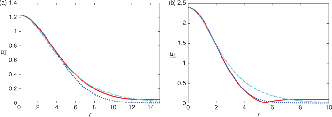
Figure 3.7 Numerical solution of nematicon equations (Eqs. 3.100 and 3.101) for |E| for Gaussian initial condition: solid line; sech fitted to numerical solution: dot-dashed line; and Gaussian fitted to numerical solution: dotted line. (a) At minimum of amplitude oscillation and (b) at maximum of amplitude oscillation. The initial conditions are a = 2.0, w = 5.0 with q = 2 and ν = 100.
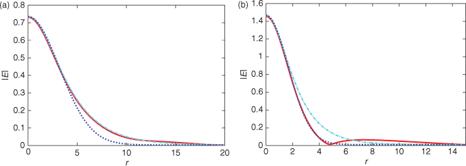
The degree of beam profile evolution as a nematicon evolves depends on the degree of nonlocality ν and the size of the amplitude oscillation. In general, as the amplitude of the oscillation increases, the beam profile changes more, resulting in greater levels of beating in the amplitude oscillation. This result is independent of the initial beam shape chosen. The other main determinant of beam shape is the nonlocality ν. This is illustrated further in Figure 3.8, for which the initial condition is a Gaussian and the nonlocality is ν = 10, which is at the lower end of the experimental range O(10)–O(100) [16, 24, 26]. It can be seen that the beam profile oscillates between a sech at an oscillation minimum and a Gaussian at a maximum. The behavior at the maximum is the same as in Figure 3.7, but at the minimum, the profile is a sech. As the nonlocality ν approaches ∞, the nematicon profile approaches a Gaussian [33]. This asymptotic behavior can be seen in the comparisons of Figures 3.6, 3.7, 3.8.
Figure 3.8 Numerical solution of nematicon equations (Eqs. 3.100 and 3.101) for |E| for Gaussian initial condition: solid line; sech fitted to numerical solution: dot-dashed line; and Gaussian fitted to numerical solution: dotted line. (a) At minimum of amplitude oscillation and (b) at maximum of amplitude oscillation. q = 2 and ν = 10.
These beam shape comparisons indicate the complex nature of the evolution of a nematicon and show that simple trial functions cannot capture all this complexity. The use of a Gaussian for the beam shape is popular because of the shape of a nematicon in the extreme nonlocal limit [33], but for the values of ν used in experiments, which are in the range O(10)–O(100) [16, 24, 26], the comparisons of this section show that a sech provides an equally good approximation. Indeed, the comparisons with modulation theory based on a sech profile shown in Figure 3.5 show that a sech gives results in good agreement with full numerical solutions. Although it may be deduced from the comparisons of Figures 3.6, 3.7, 3.8 that a Gaussian is a better approximation than a sech for ν of O(100), nematicon evolution is much more complicated than this. The best profile approximation depends on the details of the situation at hand. For example, for two-color nematicon evolution in the nonlocal limit, it was found that a Gaussian gave a good approximation to the evolution only for ν of O(1000) and greater, whereas a sech gave a good approximation for ν of O(100) [27]. The NLS soliton in one space dimension has a sech profile. The examples of this section of nematicon evolution in two space dimensions show that the shadow of this exact NLS soliton solution carries through to higher space dimensions and more intricate NLS-type equations. The examples of nematicon evolution discussed so far have the nematicon propagating on a straight-line trajectory. In Chapter 15, examples will be discussed, which have nonstraight nematicon trajectories. It is found that in many of these examples the nematicon trajectory is independent, or nearly independent, of its profile, as also found in the published literature [28, 29, 34]. As in potential technological applications of nematicons, it is their trajectories that are the important quantities and the quantities that need to be controlled [35–37], the present discussion shows that the use of trial functions based on simple profiles is a powerful technique to analyze nematicon evolution.
As previously mentioned, a popular approximation to use for the analysis of nematicon evolution is the so-called accessible soliton limit of Snyder and Mitchell [33]. This limit is essentially that of infinite nonlocality ν and in this limit the nematicon equations reduce to
P is then the conserved power of the beam and is constant. In this limit, the nematicon equations thus reduce to the linear Schrödinger's equation, so that the techniques and solutions of quantum mechanics become available. However, caution must be applied in making deductions about the evolution of nematicons in experimental situations based on the results of the Snyder–Mitchell limit. The usual range of ν in experiments is O(10)–O(100) [16, 24, 26], which, although large, is not in the “highly nonlocal” limit needed for the Snyder–Mitchell approximation. The finite values of nonlocality valid for experiments have one major consequence. The “potential” in the Schrödinger's equation (Eq. 3.138) is infinite, so that only bound states are possible. This means that any radiation shed by an evolving nematicon is trapped by the potential, so that it cannot evolve to a steady state. The beam solutions in the Snyder–Mitchell limit [33] then oscillate indefinitely, rather than shed radiation, and evolve in an oscillatory manner to a steady nematicon as for finite ν. Cell lengths in experiments are of O(1mm) and so, typically, only two or three oscillations of the beam width are observed [15, 24]. The decay of the nematicon onto the steady state is ![]() , which is very slow in the nonlocal limit. Given that it is impossible to experimentally generate an exact nematicon as an input to a cell, it is then impossible to observe an exact steady nematicon. So, although experiments appear to support the idea that the nematicon Equations (Eqs. 3.100 and 3.101) have an oscillatory “breather” solution of Snyder–Mitchell type, mathematically the nematicon equations do not possess such a solution. In general, NLS-type equations do not possess single solitary wave breather solutions [6]. Although for highly nonlocal media single solitary wave breathing solutions for NLS-type equations may appear to be steady solutions for experimentally relevant distances [38], they are not steady solutions in the mathematical sense in that they are not steady indefinitely. They will shed radiation, maybe of very low amplitude on a very long space scale, to evolve to a fixed amplitude solitary wave solution. The distance needed to see this evolution may, of course, be far longer than is experimentally feasible. Another effect of the infinite potential of the Schrödinger's equation (Eq. 3.138) is that it can suppress instabilities that arise for finite values of ν. An example of this is the “crescent vortices” of He et al. [39], which were found to be stable as solutions in the Snyder–Mitchell limit but are unstable for experimental values of ν.
, which is very slow in the nonlocal limit. Given that it is impossible to experimentally generate an exact nematicon as an input to a cell, it is then impossible to observe an exact steady nematicon. So, although experiments appear to support the idea that the nematicon Equations (Eqs. 3.100 and 3.101) have an oscillatory “breather” solution of Snyder–Mitchell type, mathematically the nematicon equations do not possess such a solution. In general, NLS-type equations do not possess single solitary wave breather solutions [6]. Although for highly nonlocal media single solitary wave breathing solutions for NLS-type equations may appear to be steady solutions for experimentally relevant distances [38], they are not steady solutions in the mathematical sense in that they are not steady indefinitely. They will shed radiation, maybe of very low amplitude on a very long space scale, to evolve to a fixed amplitude solitary wave solution. The distance needed to see this evolution may, of course, be far longer than is experimentally feasible. Another effect of the infinite potential of the Schrödinger's equation (Eq. 3.138) is that it can suppress instabilities that arise for finite values of ν. An example of this is the “crescent vortices” of He et al. [39], which were found to be stable as solutions in the Snyder–Mitchell limit but are unstable for experimental values of ν.
3.9 Conclusions
There are many nonlinear wave equations and systems of such equations that do not possess exact solitary wave solutions. Of particular relevance for this book is the system of equations governing solitary wave, or nematicon, propagation in nematic liquid crystals. It may then be thought that the only manner in which to gain insight into the dynamics of such solitary waves is through numerical solutions of the governing equations. However, it has been shown that extending Whitham modulation theory [1] results in a powerful approximate technique that allows much insight into the mechanisms governing solitary wave and nematicon evolution, as well as giving solutions in excellent agreement with numerical solutions of the governing equations, as demonstrated for the standard NLS equation and for the equations governing nematicons in a nematic liquid crystal. Indeed, Whitham modulation theory itself is an analytically sophisticated, infinite dimensional extension of multiple scales perturbation theory. It can then include higher order effects, and so can the present extension of this theory, provided that a good trial function is chosen.
As the exact solitary wave profile is unknown, modulation theory relies on assuming an appropriate profile. Although it may be thought that the results of the modulation theory would depend critically on this assumed profile, it has been shown that this is not the case, as long as the assumed profile is reasonable in that it has a solitary wave form. Numerical solutions of the nematicon equations show that the nematicon profile changes form as the nematicon evolves. A popular profile for a nematicon is a Gaussian as in the infinite nonlocality limit it can be shown that the profile is of this form [33]. However, it has been shown that for realistic experimental values of the nonlocality ν an initial Gaussian profile does not stay of this form but oscillates between a Gaussian and a more sech profile.
An added benefit of the present form of modulation theory is that it easily allows for the incorporation of the effect of the diffractive radiation shed by an evolving solitary wave. All solitary waves shed radiation in order to evolve. Without the inclusion of this radiation, the solutions from any perturbation or approximate theory cannot evolve to a steady state as there is no damping term in the equations. For nematicons, as the nonlocality ν increases, the amplitude of the shed radiation decreases, so that the nematicon takes longer to reach a steady state. This distance to reach a steady state is usually longer than the physical length of the cell containing the nematic liquid crystal.
Acknowledgments
This research was supported by the Royal Society of London under Grant No. JP090179.
Appendix 3.A: Integrals
The integrals Ii and Ii, j in the modulation equations are
3.A.1 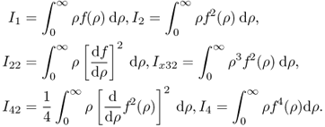
For f(ρ) = sech ρ
3.A.2 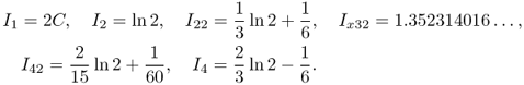
Here, C is the Catalan constant C = 0.915965594 … [31]. For f(ρ) = exp( − ρ2)
3.A.3 ![]()
The constants A and B arising in the modulation equations are
3.A.4 ![]()
Appendix 3.B: Shelf Radius
As for the NLS equation, the radius ![]() of the shelf of diffractive radiation under an evolving nematicon is determined by linearizing the modulation Equations 3.110–3.114 about the fixed point with
of the shelf of diffractive radiation under an evolving nematicon is determined by linearizing the modulation Equations 3.110–3.114 about the fixed point with
3.B.1 ![]()
where |a1| ![]() af, |w1|
af, |w1| ![]() wf, |α1|
wf, |α1| ![]() αf, |β1|
αf, |β1| ![]() βf, |g1|
βf, |g1| ![]() 1, and |σ1|
1, and |σ1| ![]() σf. In a straightforward, but tedious, calculation, it is found on eliminating all the derivatives in terms of
σf. In a straightforward, but tedious, calculation, it is found on eliminating all the derivatives in terms of ![]() and then eliminating
and then eliminating ![]() in terms of g1 that
in terms of g1 that
3.B.2 
where
3.B.3 
3.B.4 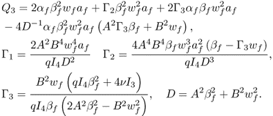
As for the NLS equation, the frequency of the simple harmonic motion equation (Eq. 3.B.2) is now matched to the steady nematicon oscillation frequency , given by Equation 3.113 with a, w, β, and α replaced by their fixed-point values. This results in the radius ![]() of the shelf of low wave number diffractive radiation under the beam being given by
of the shelf of low wave number diffractive radiation under the beam being given by
3.B.5 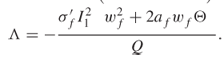
1. G. B. Whitham. Linear and Nonlinear Waves. John Wiley & Sons, New York, 1974.
2. G. B. Whitham. Non-linear dispersive waves. Proc. R. Soc. London, Ser. A, 283: 238–261, 1965.
3. J. D. Cole and J. K. Kevorkian. Perturbation Methods in Applied Mathematics. Springer-Verlag, Berlin, 1981.
4. J. Hale. Ordinary Differential Equations. Wiley Interscience, New York, 1972.
5. Y. S. Kivshar and G. Agrawal. Optical Solitons: From Fibers to Photonic Crystals. Academic Press, San Diego, CA, 2003.
6. G. L. Lamb. Elements of Soliton Theory. John Wiley & Sons, New York, 1980.
7. A. C. Newell. Solitons in Mathematics and Physics. SIAM, Philadelphia, PA, 1985.
8. D. J. Kaup and A. C. Newell. Solitons as particles, oscillators, and in slowly changing media: a singular perturbation theory. Proc. R. Soc. A, 361: 413–446, 1978.
9. C. Knickerbocker and A. C. Newell. Shelves and the Korteweg-de Vries equation. J. Fluid Mech., 98: 803–818, 1980.
10. I. M. Gelfand and S. V. Fomin. Calculus of Variations. Prentice-Hall, Englewood Cliffs, NJ, 1963.
11. J. Yang. Vector solitons and their internal oscillations in birefringent nonlinear optical fibers. Stud. Appl. Math., 98: 61–97, 1997.
12. D. E. Pelinovsky and Y. Yang. Internal oscillations and radiation damping of vector solitons. Stud. Appl. Math., 105: 245–276, 2000.
13. E. A. Coddington and N. Levinson. Theory of Ordinary Differential Equations. Krieger Pub. Co., Malabar, 1984.
14. R. L. Pego and M. I. Weinstein. Asymptotic stability of solitary waves. Commun. Math. Phys., 164: 305–349, 1994.
15. G. Assanto, M. Peccianti, and C. Conti. Optical spatial solitons in nematic liquid crystals: Nematicons. Opt. Photon. News, 14: 45–48, 2003.
16. C. Conti, M. Peccianti, and G. Assanto. Route to nonlocality and observation of accessible solitons. Phys. Rev. Lett., 91:073901, 2003.
17. C. Conti, M. Peccianti, and G. Assanto. Observation of optical spatial solitons in a highly nonlocal medium. Phys. Rev. Lett., 92:113902, 2004.
18. D. Anderson. Variational approach to nonlinear pulse propagation in optical fibers. Phys. Rev. A, 27: 3135–3145, 1983.
19. W. L. Kath and N. F. Smyth. Soliton evolution and radiation loss for the nonlinear Schrödinger equation. Phys. Rev. E, 51: 1484–1492, 1995.
20. T. Jintao, L. Hongjun, G. Cunxiao, Z. Wei, W. Yishan, and C. Guofu. Spectrum shape compression and pedestal elimination employing a Sagnac loop. Opt. Commun., 282: 74–77, 2009.
21. Q. Li, K. Senthilnathan, K. Nakkeeran, and P. K. A. Wai. Nearly chirp- and pedestal-free pulse compression in nonlinear fiber Bragg gratings. J. Opt. Soc. Am. B, 26: 432–443, 2009.
22. J. P. Gordon. Dispersive perturbations of solitons of the nonlinear Schrödinger equation. J. Opt. Soc. Am. B, 9: 91–97, 1992.
23. J. Satsuma and N. Yajima. Initial value problems of one-dimensional self-modulation of nonlinear waves in dispersive media. Prog. Theor. Phys. Suppl., 55: 284–306, 1974.
24. M. Peccianti, C. Conti, G. Assanto, A. De Luca, and C. Umeton. Routing of anisotropic spatial solitons and modulational instability in liquid crystals. Nature, 432: 733–737, 2004.
25. M. Peccianti, A. Fratalocchi, and G. Assanto. Transverse dynamics of nematicons. Opt. Express, 12: 6524–6529, 2004.
26. G. Assanto, A. A. Minzoni, M. Peccianti, and N. F. Smyth. Optical solitary waves escaping a wide trapping potential in nematic liquid crystals: modulation theory. Phys. Rev. A, 79:033837, 2009.
27. B. D. Skuse and N. F. Smyth. Interaction of two-color solitary waves in a liquid crystal in the nonlocal regime. Phys. Rev. A, 79:063806, 2009.
28. G. Assanto, B. D. Skuse, and N. F. Smyth. Optical path control of spatial optical solitary waves in dye-doped nematic liquid crystals. Photon. Lett. Poland, 1: 154–156, 2009.
29. G. Assanto, B. D. Skuse, and N. F. Smyth. Solitary wave propagation and steering through light-induced refractive potentials. Phys. Rev. A, 81:063811, 2010.
30. A. A. Minzoni, N. F. Smyth, and A. L. Worthy. Modulation solutions for nematicon propagation in non-local liquid crystals. J. Opt. Soc. Am. B, 24: 1549–1556, 2007.
31. M. Abramowitz and I. A. Stegun. Handbook of Mathematical Functions with Formulas, Graphs and Mathematical Tables. Dover Publications, New York, 1972.
32. C. García-Reimbert, A. A. Minzoni, and N. F. Smyth. Spatial soliton evolution in nematic liquid crystals in the nonlinear local regime. J. Opt. Soc. Am. B, 23: 294–301, 2006.
33. A. W. Snyder and M. J. Mitchell. Accessible solitons. Science, 276: 1538–1541, 1997.
34. B. D. Skuse and N. F. Smyth. Two-colour vector soliton interactions in nematic liquid crystals in the local response regime. Phys. Rev. A, 77:013817, 2008.
35. A. Fratalocchi, R. Asquini, and G. Assanto. Integrated electro-optic switch in liquid crystals. Opt. Express, 13: 32–37, 2005.
36. M. Peccianti, A. Dyadyusha, M. Kaczmarek, and G. Assanto. Tunable refraction and reflection of self-contained light beams. Nat. Phys., 2: 737–742, 2006.
37. A. Piccardi, A. Alberucci, U. Bortolozzo, S. Residori, and G. Assanto. Soliton gating and switching in a liquid crystal light valve. Appl. Phys. Lett., 96:071104, 2010.
38. I. Kaminer, C. Rotschild, O. Manela, and M. Segev. Periodic solitons in nonlocal nonlinear media. Opt. Lett., 32: 3209–3211, 2007.
39. Y. J. He, B. A. Malomed, D. Mihalache, and H. Z Wang. Crescent vortex solitons in strongly nonlocal nonlinear media. Phys. Rev. A, 78:023824, 2008.