
Chapter 9: Propagation of Light Confined via Thermo-Optical Effect in Nematic Liquid Crystals
Unité de Catalyse et de Chimie du Solide, Faculté des Sciences, Université d'Artois, Lens, France
9.1 Introduction
Every material is temperature sensitive, and its physical parameters are temperature dependent. The optical properties are not an exception; hence, the index of refraction depends on temperature. In terms of applications, this could generally be regarded as a drawback, as a temperature change affects the index, and thus the propagation and, eventually, the operation of the device. Fortunately, for most materials, such dependence is quite weak. The best way to characterize it is the thermal coefficient of refraction ![]() . For most manufactured glasses, this figure is around ±10−6 K−1, a few orders of magnitude larger than that for organic liquids (5 × 10⁻⁴ K−1 for acetone) and a few more for liquid crystals (10−2 K−1 for pentyl cyanobiphenyl). To give an insight of what such a figure means, let us take a textbook example: the minimum deflection of a beam by a prism. The change of that deflection is proportional to the change of the prism index of refraction. An increase of 10 K in the temperature of a prism (equilateral section) made of glass with a dn/dT = 10−6 K−1 results in a variation of the beam minimum deflection of 4 × 10⁻⁴°; for a
. For most manufactured glasses, this figure is around ±10−6 K−1, a few orders of magnitude larger than that for organic liquids (5 × 10⁻⁴ K−1 for acetone) and a few more for liquid crystals (10−2 K−1 for pentyl cyanobiphenyl). To give an insight of what such a figure means, let us take a textbook example: the minimum deflection of a beam by a prism. The change of that deflection is proportional to the change of the prism index of refraction. An increase of 10 K in the temperature of a prism (equilateral section) made of glass with a dn/dT = 10−6 K−1 results in a variation of the beam minimum deflection of 4 × 10⁻⁴°; for a ![]() four orders of magnitude larger [e.g., 10−2 K−1 in nematic liquid crystal (NLC)], this variation would be of 4°, which is no longer insignificant. As usual in optics, this thermal effect would be detectable if the change in phase shift or equivalently in optical path (index × propagation length) would be large enough. For instance, although the atmosphere index is very close to 1 and has a very small
four orders of magnitude larger [e.g., 10−2 K−1 in nematic liquid crystal (NLC)], this variation would be of 4°, which is no longer insignificant. As usual in optics, this thermal effect would be detectable if the change in phase shift or equivalently in optical path (index × propagation length) would be large enough. For instance, although the atmosphere index is very close to 1 and has a very small ![]() , atmospheric thermal fluctuations or mirage can be clearly visible! The thermal effect occurs whatever the origin of the temperature gradient. In other words, any temperature gradient induced by a beam would affect its own propagation, as for other nonlinearities. The effects associated with the thermal nonlinearity will be perceivable if the thermal coefficient of refraction or/and the induced temperature gradient is large enough. To observe these effects, the experimental setup is, in principle, simple: the index gradient is generated by local heating because of absorption of a nonuniform intense beam. In this chapter, we explore this capability: a beam with a nonuniform intensity (Gaussian) propagates through a medium with a large thermal coefficient of refraction, namely, an NLC. Before going into this topic, let us make some general and essential comments. The first two deal with the semantics of the expressions “nonlinear optics” and “optical soliton,” and the third contains more physics.
, atmospheric thermal fluctuations or mirage can be clearly visible! The thermal effect occurs whatever the origin of the temperature gradient. In other words, any temperature gradient induced by a beam would affect its own propagation, as for other nonlinearities. The effects associated with the thermal nonlinearity will be perceivable if the thermal coefficient of refraction or/and the induced temperature gradient is large enough. To observe these effects, the experimental setup is, in principle, simple: the index gradient is generated by local heating because of absorption of a nonuniform intense beam. In this chapter, we explore this capability: a beam with a nonuniform intensity (Gaussian) propagates through a medium with a large thermal coefficient of refraction, namely, an NLC. Before going into this topic, let us make some general and essential comments. The first two deal with the semantics of the expressions “nonlinear optics” and “optical soliton,” and the third contains more physics.
Although this chapter deals with effects observed in NLC, it should be noticed that thermo-optic effects—lensing, self-focusing, and defocusing of high-power laser beams—have been observed in other media (e.g., in gas) and modeled long ago [1–4]. Restricting our attention to NLC media, we have to consider two different geometries: thin and thick samples. In other words, does the beam propagate within the medium over a short or long distance? In the case of a thin sample, the beam crosses the sample and experiences classical nonlinear effects, such as self-phase-modulation and bistability [5] or some lens effect (self-focusing), which has been studied quite early [6, 7] and used—for instance—to characterize the material [8]. These two geometries—thin and thick samples—can be addressed from another point of view: the beam travels either across (thin samples) or along (thick samples) the NLC boundary: in other words, not only the propagation distance but also the nematic elasticity is different. However, as this chapter deals with the thermal effect and not with the orientational effect, we do not consider this aspect: it is discussed in the other chapters of this book. We thus limit our attention to beams propagating a long distance through an NLC and how the large dependence of the index of refraction on temperature coupled to a nonuniform intensity of the beam affects its propagation. In Section 9.2, we report experimental observations on nonlinear propagation, and in Section 9.3, we focus on the methods proposed to analyze and characterize the effects and, among others, the nonlocality. We then compare, in Section 9.4, the thermal response with the orientational one: do they act with the same strength? Finally, we explore the potential applications of the thermal dependence (Section 9.5).
9.2 First Observation in NLC
Generally speaking, three conditions are required to observe the temperature-induced confined propagation of a beam. They are sketched in Figure 9.1.
Figure 9.1 Principle of thermal nonlinear propagation: the beam intensity should be nonuniform, it should propagate in an absorbing medium, and the thermal coefficient of refraction dn/dT should be large. The nonuniform intensity generates a hotter region (on-axis of propagation in this sketch), which in turn generates an index gradient (focusing for dn/dT > 0, solid line; defocusing for dn/dT < 0 dashed line). Source: Reprinted from Reference 9. Copyright 2008, with permission from the Optical Society of America.
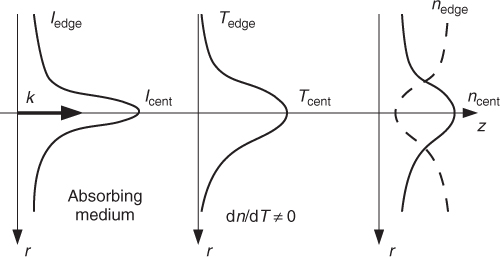
First, the optical intensity should be spatially nonuniform. Second, the medium in which the light propagates should be slightly absorbing: the regions where the optical field is large absorb more and thus heat more than those where there is no optical field. A thermal equilibrium will be reached, which should ensure a stable temperature gradient. The third condition to be fulfilled concerns the medium as well: it should have an index that depends on temperature to transform the temperature gradient into an index gradient large enough to act in a detectable manner on the beam. As already mentioned in the introduction, NLC has one of the largest thermal coefficients, which can be either positive (focusing medium) or negative (defocusing medium).
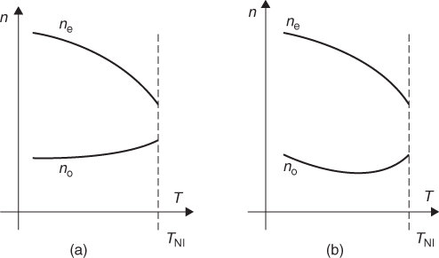
In the geometries explored, the first condition is usually achieved by using a Gaussian beam, which is easy to handle, control, and characterize before and after nonlinear propagation. The second condition—to render the medium slightly absorbing—is fulfilled by adding a very small amount of a dye to the liquid crystal. A concentration of a few 0/00 is enough to induce the required absorption while preserving the nematic nature of the mixture. The temperature of the phase transition is also slightly modified, the indices of refraction and their temperature dependence being practically unchanged. To fulfill the third condition, the choice of liquid crystals is almost obvious, because of the very large temperature dependence of their indices. However, there are several possible geometries. Indeed, while dealing with liquid crystals we deal with anisotropic media; hence, the two principal indices of refraction do not behave in the same way with temperature. Let us first recollect this feature. As shown in Figure 9.2, the extraordinary index always decreases with temperature; on the contrary, the ordinary index may increase (which is the case in most NLCs), or have a minimum.
Figure 9.2 Temperature dependence of refractive index in nematic liquid crystals. The extraordinary index is always decreasing with temperature, whereas the ordinary one can be either increasing [(a); e.g., 5CB, Merck], or going through a minimum [(b); e.g., PCH & mixture of PCH5 + PCH7, Hoffmann-La Roche [10, 11]). TNI is the clearing point, the temperature above which the material turns to be a standard isotropic liquid.
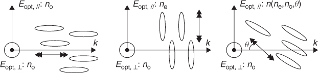
It is beyond the scope of this chapter to detail the physical reasons for such behavior: the reader may refer to the appropriate bibliography [10–14]. Whatever the chosen liquid crystal, the polarization of the beam becomes an essential parameter to be controlled in the experiments. The simplest case consists in propagating a linearly polarized beam, exciting one of the two eigenmodes of the birefringent material. The extraordinary component experiences defocusing, whereas the ordinary component focuses, provided that the ordinary index increases with temperature (Fig. 9.2a). The geometries that clearly separate the two linear eigen polarizations are shown in Figure 9.3. Any intermediate situation might be explored, although more tricky to analyze and use.
Figure 9.3 Geometries that allow exciting separately the two eigenmodes (ordinary and extraordinary waves) in NLC. The ellipses stand for the NLC director—averaged molecular alignment. The optic axis is marked with a double black arrow. The index of refraction is indicated for each optical field component.
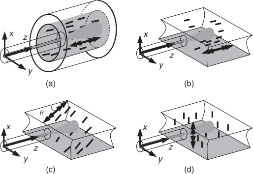
Most of the experiments on thermally induced nonlinear propagation have been performed using a mixture of pure 5CB (Merck) and anthraquinone dye (AQ1) at low concentration (1/00, w/w). The real part of the index of refraction was measured for that mixture, using a total internal reflection (TIR) setup and was found to be practically identical to that of the pure material (no = 1.53 at 633 nm). Its temperature dependence looks like the case plotted in Figure 9.2a: the thermal coefficient of refraction is always positive and, provided that the correct polarization is used, the beam would be self-focused. The thermally induced nonlinear propagation has been tested under the geometries illustrated in Figure 9.3. The mixture is confined either in a capillary tube (inner diameter: 250 μm) or in a planar cell (thickness around 125 μm). The alignment of the nematic is obtained in both cases by a conventional technique (rubbed polymer coating), and is checked by visual inspection with an optical microscope. The beam under study (CW laser beam at 633 nm or 532 nm) was injected via an optical fiber directly inserted in the NLC sample. The fiber was either simply cleaved (beam waist: 3 μm) or tapered (beam waist:10 μm). The setup geometries are shown in Figure 9.4.
Figure 9.4 The four explored geometries. The geometries sketched in (a) and (b) are equivalent: only the ordinary index is involved. The NLC alignment is parallel to the plane yz in both cells (a) and (b). The optic axis is tilted away from the direction of propagation z in cell (c). The optic axis is parallel to the x-direction in cell (d) (homeotropic alignment). The ordinary index is involved for an input beam polarization parallel to y in all cells. Source: Reprinted from Reference 15. Copyright 2001, with permission from Elsevier.
The first observation of long-distance thermally induced nonlinear beam propagation in NLC was reported in 1998 [16]. Schematically, as the input beam power is increased from 0 to around 6 mW, two regimes are observed. The first regime starts at around 4 mW: the beam self-focuses and remains collimated (equivalent to a spatial optical soliton) practically up to 6 mW. This is the input power at which the second regime is observed: a well-collimated beam, with a length that linearly and reversibly depends on the input power. As the input power is increased, the length increases; as the input power is decreased, the length decreases. These two regimes are shown in Figure 9.5. Further studies were undertaken to better understand these results. Varying the dye concentration [16] or the birefringence [17] does not change the sequence of events described earlier, it just changes the optical powers at the onset of the regimes. The capillary geometry (Fig. 9.4a) or the equivalent cell geometry (Fig. 9.4b) yield the same sequence, although these two geometries have a different boundary and thus a different heat flow [15]. The geometry in Figure 9.4c, which is polarization dependent, was checked as well [15]. As expected for large θ angle (Fig. 9.15), the extraordinary beam is clearly defocused and the ordinary one is collimated, as shown in Figure 9.6.
Figure 9.5 Sequence of events observed as the input power is increased. (a) Normal diffraction, (b) self-trapped beam, and (c) isotropic tube. Source: Reprinted from Reference 18. Copyright 2004, with permission from the American Institute of Physics.
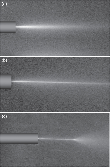
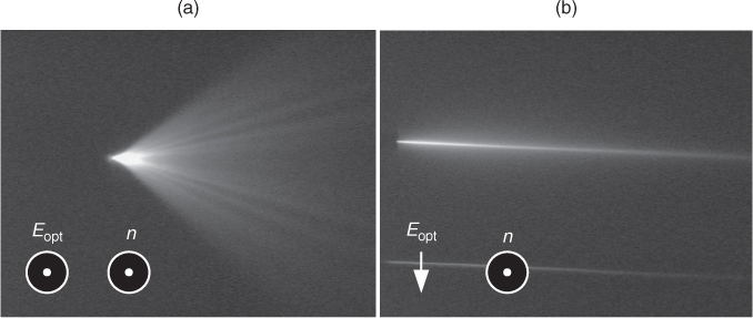
Figure 9.6 Cell with a homeotropic alignment (geometry of Figure 9.4d). The optic axis ![]() is perpendicular to the plane of the figure. (a) The optical beam excites the extraordinary component and is defocused. (b) The optical beam excites the ordinary component and is collimated (the input waist of the beam is 3 μm, and the propagation distance is about 1 mm). Source: Reprinted from Reference 15. Copyright 2001, with permission from Elsevier.
is perpendicular to the plane of the figure. (a) The optical beam excites the extraordinary component and is defocused. (b) The optical beam excites the ordinary component and is collimated (the input waist of the beam is 3 μm, and the propagation distance is about 1 mm). Source: Reprinted from Reference 15. Copyright 2001, with permission from Elsevier.
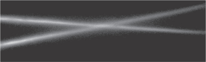
The low power regime was identified as a solitonlike regime, the second regime as an isotropic tube. These results are detailed in the next section. Let us mention two results that bring us to the conclusion that we are dealing with a solitonlike behavior. First, it was checked that two solitons crossing their paths do not change their propagation: this is shown in Figure 9.7 [15]. Second, the set of two coupled equations that rule the process were numerically solved and showed that a solitonlike regime can be excited by a purely thermal effect [19].
Figure 9.7 Cell with a homeotropic alignment (geometry of Figure 9.4d). The optic axis is perpendicular to the plane of the figure. For both beams, the polarization is in the plane of the figure and excites the ordinary component. The beams are collimated and keep propagating after crossing their paths.
To summarize these observations, as the input optical power is increased, the beam propagates normally (usual divergence) up to some value, say Ps, and then it starts to self-focus and is collimated to form a quasisoliton. At a slightly larger input power, say Pi, a phase transition occurs; the light is trapped in a tube of a nematic material that has turned to the isotropic phase. The length of that tube reversibly depends on the input optical power. The values of powers Ps and Pi depend on the actual sample and geometry. This scenario is the result of several experiments that were undertaken to point out the main parameters driving the process: they are detailed in the next section.
9.3 Characterization and Nonlocality Measurement
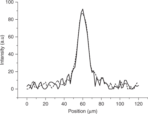
The observations mentioned earlier give rise to several questions: is the beam really well collimated (a soliton)? At which input power does the phase transition really start? A related issue is can the temperature gradient—in other words, the nonlocality—be controlled? How do two solitons behave when they are copropagate and close to each other? To answer these questions, several experiments were conducted, aiming at better characterizing the nonlinear propagation. To check how good the collimation is, the most direct approach consists in performing an image analysis: it is straightforward to get the intensity profile of a cross section of the beam, at different distances from the beam input. As shown in Figure 9.8, the radial distribution of the intensity is unchanged when measured at two different locations, 400 μm away from each other [20]. Besides the collimation confirmation, this image analysis gives the order of magnitude for the radius of the self-written waveguide; however, what is obtained this way is just an integrated value of the scattered light and should be considered with caution.
Figure 9.8 Radial intensity profiles obtained from Figure 9.5b at two positions 400 μm away from one another (dashed line: entrance; solid line after 400 μm of propagation). Source: Reprinted from Reference 19. Copyright 2000, with permission from the American Institute of Physics.
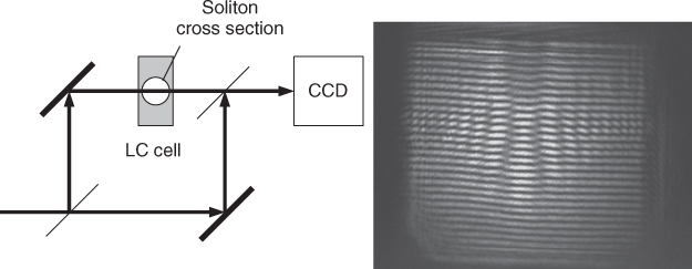
Another way to check the collimation relies on interferometry. The cell is placed in a Mach–Zehnder interferometer, as shown in Figure 9.9 [21]. The fringe pattern reveals the disturbance created by the temperature gradient. Such an interferometric technique can be used whatever the origin of the index change, thermal or orientational. Indeed, a numerical method was developed to extract the index change from such a fringe pattern [22].
Figure 9.9 Mach–Zehnder type apparatus to measure index distribution across the NLC cell. The soliton is launched perpendicular to the drawing. The photo shows an example of what is captured by the CCD camera. Such an approach can be used for any index change, either thermal or orientational. Source: Reprinted from Reference 21. Copyright 2005, with permission from SPIE.
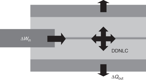
Although these two methods to analyze the collimated regime are integrated methods (integrated scattered light for the image analysis and integrated phase shift for the interferometric technique), the integration is the same for an image analysis performed at the beginning of the propagation or away from it. It is therefore appropriate to state that the beam is collimated as the intensity profile is found to be constant along the propagation direction. The second question that was addressed aims at clarifying the onset of the phase transition. This issue deals more with heat transfer than with optics. However, it turns out that the understanding of this point has a direct consequence on the optics of the problem. It allows for a better control of the induced temperature, that is, index gradient. In other words, it allows controlling the nonlocality. Let us sketch the process. As shown in Figure 9.10, the beam continuously brings some energy into the medium, which absorbs and locally heats up. This heat is expelled in every direction. The induced temperature distribution will depend on the different parameters of the sample such as heat capacity of the various components, input energy, and the overall geometry that rules the heat exchange with the surrounding. Accounting for the fact that the heat diffusion process is quite slow, the temperature, and hence the index distribution, will be robust with respect to beam intensity fluctuations faster than the diffusion characteristic time. Therefore, by using a chopped laser beam with the right characteristic times, it should be possible to control the input energy.
Figure 9.10 The input beam energy Win is partially transformed into heat, which is expelled out of the sample in every direction. In the case of dye-doped NLC, the heat flow is anisotropic.
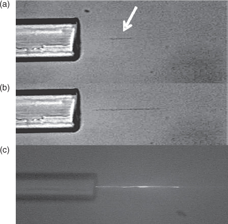
Using a laser pulse of 60 μs duration with a 500 μs repetition rate, slowly increasing the total power, it was possible to control the heat exchange and spot out the onset of the phase transition, as shown in Figure 9.11 [18].
Figure 9.11 The onset of phase transition. As the optical input power increases, the phase transition starts a few micrometers away from the input fiber (a: black line with white arrow). Then the isotropic tube enlarges symmetrically from that point (b). As the isotropic phase reaches the fiber, the tube extends to its end (c). Source: Reprinted from Reference 18. Copyright 2004, with permission from the American Institute of Physics.
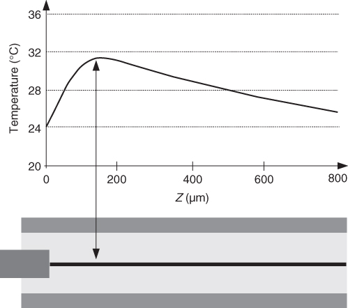
This scenario is confirmed by the numerical calculation of the temperature distribution in the cell [18]. The hottest point in the cell, that is, where the phase transition will most likely start, is found to be on the propagation axis (which is obvious) but a bit away from the fiber source, as shown in Figure 9.12. This is in agreement with the experimental result: 150 μm calculated and 180 μm measured in Figure 9.11 (top). This is a consequence of the fact that the fiber heat conductivity is higher than in NLC. The heat transfer is symmetrically distributed in the transverse direction, whereas the fiber breaks up the symmetry in the longitudinal direction. This result is consistent with the one found for another geometry [23].
Figure 9.12 On-axis temperature distribution, obtained from finite element calculation in a cell as sketched at the bottom. The hottest point is found to be at 150 μm (black arrow). Source: Reprinted from Reference 18. Copyright 2004, with permission from the American Institute of Physics.
The method of controlling the input energy by chopping the input beam can be used to control the temperature gradient in the self-collimated regime. In other words, it allows to control the nonlocality, which in our case is directly linked to the temperature gradient size as compared to the one of the input beam. Moreover, the optical molecular reorientation being a slow process, it is possible to control the nonlocality induced by this process as well, provided the repetition and duration of the pulses are not too small compared to the elastic response time that drives the reorientational process.
As the nonlocality can be somehow controlled, can it be measured? In the system described herein, the nonlocality can be characterized by comparing the nonlinear effect, namely, the index distribution, with the cause, namely, the beam width. Assuming a soliton regime, the beam width (Wb, soliton waist) and the induced index profile (Wn) remain constant along the propagation direction. The ratio Wn/Wb may be a measure of the nonlocality. One way to get an estimate of this figure consists in measuring the beam waist from the profile, as shown in Figure 9.8, and the index profile from a fringe pattern such as the one shown in Figure 9.9. In the reported experiments, the ratio is estimated to be around 2–3. Actually, although the approach sounds simple, this figure should be considered very cautiously. As already mentioned, the obtained intensity profile is an integration of the scattered light, whereas the index profile is an integration of the phase shift across the cell thickness. Thus the obtained waists are not the actual values and, more importantly, the integrations are quite different in nature for both measurements; hence, strictly speaking, they cannot be compared.
Another way to get an estimate of the induced index gradient consists in modeling the experiment.
The nonlinear propagation is modeled by two partial differential equations: one for the propagation, which is easily reduced to the scalar Helmholtz (Eq. 9.1) and the other for the heat diffusion process, which is a classical Fourier process (Eq. 9.2). These two equations are coupled via the temperature dependence of the ordinary index of refraction (Eq. 9.3). In terms of the scalar field Ψ, the propagation constant β, the wave number k, the ordinary index of refraction n(T), and the thermal constants, absorption α and thermal diffusion κ, of the material, these equations read
The coefficients a, b, and c in the thermal dependence of n (Eq. 9.3) were obtained from experimental values in 5CB [24]. The set of equations was numerically solved, yielding an index profile of around 15 μm in size, close to the one measured from interferometry [19]. The method that yields a good estimation of the ratio Wn/Wb consists in looking at the interaction between two self-waveguides. The geometry is illustrated in Figure 9.13.
Figure 9.13 Geometry of the experiment of mutual deflection of solitons used to measure the index distribution. The optic axis ![]() is perpendicular to the figure; the polarization of both beams is parallel to the plane of the figure.
is perpendicular to the figure; the polarization of both beams is parallel to the plane of the figure.
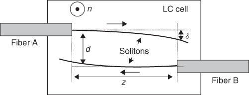
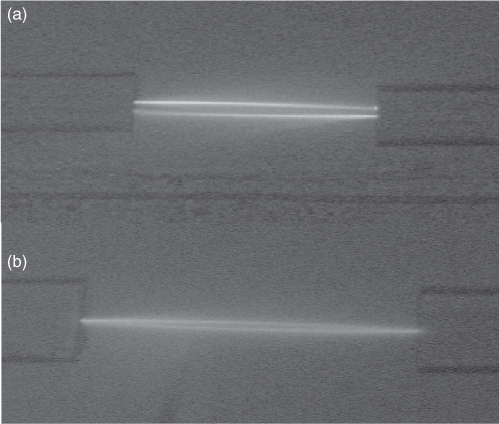
Two fibers launch two counter-propagating solitons. The fibers can be displaced in order to vary the distance between the two beams and the two fibers (d and z, Fig. 9.13). A camera is set above the cell, which captures the scattered light. One soliton is launched first (from fiber A, Fig. 9.13): it travels straight (dashed line, Fig. 9.13). Then the second one is launched: it travels through the index gradient created by the first soliton and creates an extra index gradient that disturbs the first soliton trajectory: both solitons are bent, and the measurement of the deflection (solid lines, δ, Fig. 9.13) is the signature of this mutual influence. The deflection was measured using image analysis, together with the acquired beam profiles (Fig. 9.14). Assuming that a soliton behaves like a ray, the trajectory is a matter of the eikonal equation (Eq. 9.4) that describes the path of a light beam in an inhomogeneous medium characterized by index n(r):
Figure 9.14 Example of mutual interaction of two counter-propagating solitons, for a separation between fibers of 30 μm (a) and 10 μm (b). Source: Reprinted from Reference 21. Copyright 2005, with permission from SPIE.
From experimental observations, the paraxial approximation applies and Equation 9.4 reduces to
9.5 ![]()
From the knowledge of the temperature dependence of the ordinary index and an estimate of the temperature decrease along the propagation, ![]() can be evaluated over the total length of propagation. The experimental evaluation of
can be evaluated over the total length of propagation. The experimental evaluation of ![]() is derived from the measurement of δ for different distances d between the fibers (Fig. 9.13) and leads to the determination of the radial index variation
is derived from the measurement of δ for different distances d between the fibers (Fig. 9.13) and leads to the determination of the radial index variation ![]() [25].
[25].
Solving this equation, it was possible to retrieve the index profile [25]. The ratio Wn/Wb is reported to be around 3. The actual value of this figure is most likely larger as the found beam waist is, once again, an integration; conversely, the index profile is correct, although not very accurate because it is calculated from rough measurements.
These methods to characterize the soliton are not process dependent; this means that they can be used for a soliton generated by the reorientation of the NLC (nematicon) [26]. To fully characterize the nonlinear propagation, it would be interesting to compare the two processes that may induce a soliton in a liquid crystalline material, that is, thermal and orientational. The next section addresses this issue.
9.4 Thermal Versus Orientational Self-Waveguides
As it was pointed out in Section 9.2, the extraordinary index always decreases with temperature. In an experiment dealing with nematicons, it is the extraordinary component that is involved and a temperature change would play a defocusing role, counteracting the orientational focusing effect. This is why the NLC used in these experiments is carefully chosen (most of the times E7) to avoid such counteracting effect. On the contrary, it might be interesting to compare both effects: is it possible to excite simultaneously the two kinds of solitons, and which one is stronger? At first glance, the coexistence of both solitons looks unlikely; however, it was possible to observe it and, in addition, to show that the orientational effect is much stronger than the thermal one, that is, it requires a lower input beam intensity to be excited [9]. The geometry used to obtain those two solitons is the one in Figure 9.4c. The polarization of the input beam is linear and tilted with respect to the plane of the figure: within the NLC, both ordinary and extraordinary components are excited. The intensity of each component depends on the angle of the input polarization, which can be varied. In such a scheme, the actual extraordinary index n is a well-known function of ne, no, and θ, the angle between the optic axis and the direction of propagation
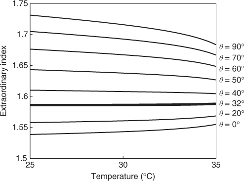
Accounting for the opposite behavior of each of the principal indices ne and no, one expects some value for the tilt angle θ at which the temperature dependence for the resulting extraordinary index is strongly reduced. Indeed, for the employed NLC (5CB), the resulting extraordinary index is practically insensitive to temperature for an angle of 32°, as shown in Figure 9.15.
Figure 9.15 Temperature dependence of the extraordinary index for several values of the angle θ between the optic axis and the direction of propagation. For θ = 32°, the index is practically independent on T (calculated using values of ne and no from Reference 24). Source: Reprinted from Reference 9. Copyright 2008, with permission from the Optical Society of America.
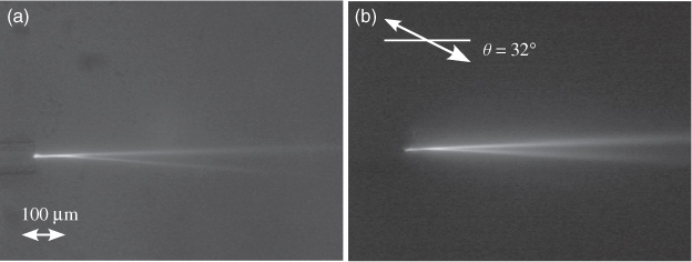
As shown in Figure 9.16, obtained using 5CB slightly doped with the dye AQ1, in the geometry 9.4c, with an angle θ set to 32°, the coexistence of an ordinary “thermal” soliton with an “orientational” extraordinary soliton is possible. Regarding the tolerance on the angle θ: how far from the calculated value θ = 32° can the two solitons still coexist? Surprisingly, the coexistence was observed over a large range of tilt angles. However, looking more carefully at the role of each of the contributions, thermal and orientational, this experimental result is in agreement with a very simple picture, as developed in Reference 9 and briefly summarized later. The index gradient for the extraordinary component is generated by a change in the tilt angle, due to optical reorientation, and by a change of temperature, due to local absorption. In a direction transverse to propagation, the gradient is expressed as
9.7 ![]()
Figure 9.16 Coexistence of “thermal” and “orientational” solitons [(a) P = 2.4 mW], free propagation [(b), P = 1.5 mW] (the input waist of the beam is 3 μm and the distance of propagation is about 1 mm). Source: Reprinted from Reference 9. Copyright 2008, with permission from the Optical Society of America.
This can be understood as a temperature gradient weighed by a thermal portion ![]() added to an orientational gradient
added to an orientational gradient ![]() , weighed by an orientational portion
, weighed by an orientational portion ![]() . The dependence of n on T is known for the material 5CB [24], and the dependence of n on the angle θ is given by Equation 9.6. It is therefore possible to calculate each of these two weights and to look for an overall positive index gradient for different values of the ratio between orientational and thermal gradients. It turns out that the coexistence of the two solitons was observed for tilt angles as large as 60°; this means that, after numerical calculation, although the temperature gradient is around 100 times larger than the orientational one, the orientational weight is larger than the “thermal” weight and, on the whole, gives rise to a positive index gradient for most tilt angles. In other words, the orientational effect is much stronger than the thermal one.
. The dependence of n on T is known for the material 5CB [24], and the dependence of n on the angle θ is given by Equation 9.6. It is therefore possible to calculate each of these two weights and to look for an overall positive index gradient for different values of the ratio between orientational and thermal gradients. It turns out that the coexistence of the two solitons was observed for tilt angles as large as 60°; this means that, after numerical calculation, although the temperature gradient is around 100 times larger than the orientational one, the orientational weight is larger than the “thermal” weight and, on the whole, gives rise to a positive index gradient for most tilt angles. In other words, the orientational effect is much stronger than the thermal one.
9.5 Applications
Any application based on a temperature-dependent effect would be not too easy to implement, as it would require a severe external temperature control to ensure that the exploited effect not be perturbed by external parameters. However, at least two potential applications can be mentioned for thermal optical solitons. The first one is based on the bent waveguide, whereas the second can be used for fluorescence recovery.
9.5.1 Bent Waveguide
We developed an experiment to test the transmission properties of this confining structure. Using the same setup as the one in Figure 9.14, we launched two isotropic channels in opposite directions by injecting laser beams (λ = 532 nm) in two optical fibers, slightly tilted with respect to each other. The distance between the fibers along the z-axis was in the order of 400 μm. As stated earlier, it is possible to adjust the length of the isotropic channels by carefully adjusting the input power: this was done for each source in order to join the two channels (Fig. 9.17).
Figure 9.17 Isotropic bent channel obtained by joining two counter-propagating isotropic tubes.
A low power He–Ne beam (probe) was injected in one fiber and detected at the output of the other one. We could thus check whether the bent structure could guide light. Using micropositioners, the angle between the fibers was precisely adjusted. By varying this angle, we checked the maximum bending of the isotropic channel that still allowed for the transmission of the probe. As the angle was too large, the probe beam “leaked” out of the first channel and was no longer guided to the second fiber. The limit was imposed by the index variation induced by the nematic/isotropic phase transition. We experimentally found that the probe signal is transmitted through the bent structure for a maximum angle of 7°. A rough calculation, based on total internal refraction considerations, shows that this limit angle yields an index variation of about 10−2, consistent with the known values for the considered material (T = 35.3°C, λ = 632.8 nm, no = 1.548, ne = 1.585).
9.5.2 Fluorescence Recovery
Up to now, spatial optical solitons have been mostly studied for potential applications in steering and routing of light beams [27, 28]. Recently, we proposed another use based on the enhancement of fluorescence recovery. The fluorescence signal is often weak and, as a result, its enhancement becomes a real challenge. When a spatial soliton propagates in an active medium, the corresponding luminescence will be partly trapped within the self-induced waveguide and driven to its output. We demonstrated the feasibility of such concept by comparing the collected fluorescence signal of a dye mixed in an NLC host, excited either by a freely expanding beam or by a spatial soliton. The setup is similar to the one we used for soliton interactions (Fig. 9.18).
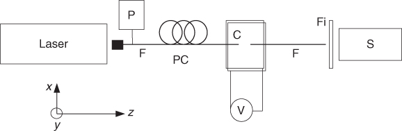
Figure 9.18 Experimental setup (P, power meter; PC, polarization controller; F, fibers; C, LC cell; Fi, notch filter; S, spectrometer; V, voltage generator). Source: Reprinted from Reference 29. Copyright 2010, with permission from the American Institute of Physics.
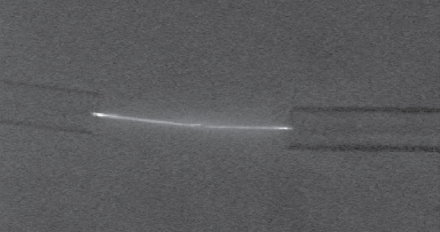
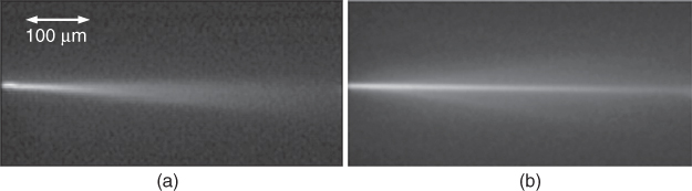
Two single-mode fibers, facing each other, are introduced in the bulk of an NLC cell. A CW pump beam (λ = 532 nm) emitted from the left fiber propagates either freely or collimated (soliton), depending on the input power. The right fiber collects and transmits the light to a spectrometer after passing through a notch filter, to eliminate the pump. The material under study is a mixture of NLC 5CB and Quinizarin (0.1% in weight). This low concentration was chosen in order to obtain a weak signal of fluorescence and thus to test the sensitivity of the method. The collected spectra of fluorescence between 400 and 1000 nm are compared in both cases. The two regimes of propagation are shown in Figure 9.19: a normally diverging beam (Fig. 9.19a) and a soliton (Fig. 9.19b). The transverse size of the soliton was estimated by image analysis as 5.6 ± 0.5 μm, which corresponds to a diffraction length zR of around 200 μm.
Figure 9.19 Laser beam propagating across the liquid crystal cell. (a) Pin = 1.5 mW (free propagation), (b) Pin = 3.5 mW (soliton). Source: Reprinted from Reference 29. Copyright 2010, with permission from the American Institute of Physics.
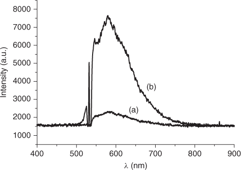
The first experiment consisted in increasing the pump power from 0.5 mW up to 5 mW, maintaining constant the interfiber distance (d = 500 μm). The soliton regime occurred above 3.5 mW. Examples of spectra recorded in the free regime and in the soliton regime are shown in Figure 9.20. The collected intensity is four times larger in the case of a soliton than in the linear case, taking into account the pump increase.
Figure 9.20 Fluorescence spectrum for (a) Pin = 1.5 mW (free beam) and (b) Pin = 3.7 mW (soliton), d = 500 μm. Source: Reprinted from Reference 29. Copyright 2010, with permission from the American Institute of Physics.
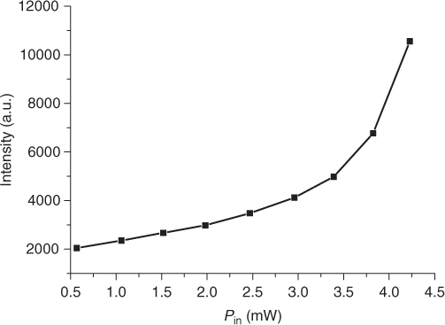
The evolution of the maximum intensity of fluorescence is plotted against input power in Figure 9.21. For low pump powers, the maximum intensity of the fluorescence increases linearly with pump power. At around 2.2 mW, thermal self-focusing starts and the collected intensity no longer varies linearly with the input power. For larger pump power, the soliton regime starts and the signal increases linearly once again, with a higher slope than before. For input pump powers higher than 5 mW, the liquid crystal heats too much and, when approaching the isotropic phase, becomes highly unstable. Changing the distance d between the fibers, from 125 to 500 μm, we observed that the fluorescence signal stayed quite constant for the soliton regime, whereas it decreased, as expected, in the free propagation case [29]. By this result, we demonstrated the possibility of using spatial solitons as a local probe of fluorescence in liquid suspensions.
Figure 9.21 Evolution of the maximum intensity of the fluorescence spectrum (λ = 590 nm) versus input pump power for a constant fiber distance (d = 500 μm). The soliton regime starts around 3.5 mW, the signal increases quite sharply. Source: Reprinted from Reference 29. Copyright 2010, with permission from the American Institute of Physics.
9.6 Conclusions
Besides the very well-known display applications, NLCs should be considered as a very good test material to investigate complex electromagnetic wave propagation. In this chapter, we focused on the strong temperature dependence of refractive indices, yielding to nonlinear propagation, especially self-waveguiding or quasispatial optical solitons. Different experiments were set up to characterize such confined propagation, the essential parameter being the induced index profile. In terms of applications, thermo-optical solitons are good candidates not only for optical routing but also for locally probing optical properties of material. Their strong nonlocality, associated with the diffusive properties of the thermo-optic effect, gives them good stability when they are coupled to optical fibers. The waveguide properties of the solitons were also exploited to enhance the recovery of a fluorescence signal from a mixture of dye and liquid crystals. Further investigations could be carried out in this direction, for example, concerning the luminescence of colloids of nanoparticles in NLC samples.
1. J. P. Gordon, R. C. C. Leite, R. S. Moore, S. P. S. Porto, and J. R. Whinnery. Long transient effects in lasers with inserted liquid samples. J. Appl. Phys., 36(1):3–8, 1965.
2. S. A. Akhmanov, D. P. Krindach, A. P. Sukhorukov, and R. V. Khokhlov. Nonlinear defocusing of lasers beams. JETP Lett., 6(2):38–42, 1967.
3. S. A. Akhmanov, D. P. Krindach, A. V. Migulin, A. P. Sukhorukov, and R. V. Khokhlov. Thermal self actions of laser beams. IEEE J. Quantum Electron., 4(10):568–575, 1968.
4. F. W. Perkins and E. J. Valeo. Thermal self-focusing of electromagnetic waves in plasmas. Phys. Rev. Lett., 32(22):1234–1237, 1974.
5. P. Y. Wang, H. J. Zhang, and J. H. Dai. Laser-heating induced self-phase modulation, phase transition and bistability in nematic liquid crystals. Opt. Lett., 13(6):479–481, 1988.
6. V. Volterra and E. Wiener-Avnear. CW thermal lens effect in thin layer of nematic liquid crystal. Opt. Commun., 12(2):194–197, 1974.
7. V. Volterra and E. Wiener-Avnear. Laser induced isotropic holes in nematic liquid crystals. Appl. Phys. A, 6(2):257–259, 1975.
8. H. Ono, K. Takeda, and K. Fujiwara. Thermal lens produced in a nematic liquid crystal. Appl. Spectrosc., 49(8):1189–1192, 1995.
9. M. Warenghem, J.-F. Blach, and J.-F. Henninot. Thermo-nematicon: an unnatural coexistence of solitons in liquid crystals? J. Opt. Soc. Am. B, 25(11):1882–1887, 2008.
10. J. Li, S. Gauzia, and S. T. Wu. High temperature-gradient refractive index liquid crystals. Opt. Express, 12(9):2002–2010, 2004.
11. M. Schadt and F. Muller. Class specific elastic, viscous, optical and dielectric properties of some nematic liquid crystals and correlation with their performances in twisted nematic displays. Rev. Phys. Appl., 14:265–274, 1979.
12. R. Dabrowski, J. Dziaduszek, Z. Stolarz, and J. Kedzierski. Liquid crystalline material with low ordinary index. J. Opt. Technol., 72(9):662–667, 2005.
13. I. C. Khoo and F. Simoni. Physics of Liquid Crystalline Materials. Gordon & Breach, London, pp. 365–392, 1991.
14. P. G. de Gennes, and J. Prost. The Physics of Liquid Crystals. 2nd edn. Oxford University Press, London, 1995.
15. J.-F. Henninot, M. Debailleul, F. Derrien, G. Abbate, and M. Warenghem. (2D+1) Spatial optical solitons in dye doped liquid crystals. Synthetic Met., 124:9–13, 2001.
16. M. Warenghem, J.-F. Henninot, and G. Abbate. Non linearly induced self waveguiding structure in dye doped nematic liquid crystals confined in capillaries. Opt. Express, 2(12):483–490, 1998.
17. M. Warenghem, J.-F. Henninot, and G. Abbate. From Bulk Janossy effect to nonlinear self wave-guiding spatial soliton in dye-doped liquid crystal. J. Nonlin. Opt. Phys., 8(3):341–360, 1999.
18. J.-F. Henninot, M. Debailleul, R. Asquini, A. d'Alessandro, and M. Warenghem. Self-waveguiding in an isotropic channel induced in dye-doped nematic liquid crystal and a bent self-waveguide. J. Opt. A: Pure Appl. Opt., 6:315–323, 2004.
19. F. Derrien, J.-F. Henninot, M. Warenghem, and G. Abbate. Thermal (2D+1) spatial optical soliton in dye doped liquid crystal. J. Opt. A: Pure Appl. Opt., 2:332–337, 2000.
20. M. Warenghem, J.-F. Henninot, F. Derrien, and G. Abbate. Thermal and orientational 2D+1 spatial optical solitons in dye doped liquid crystals. Mol. Cryst. Liq. Cryst., 373:213–225, 2002.
21. M. Warenghem, J.-F. Henninot, and J.-F. Blach. Measurement, control and use of non-locality in some liquid crystal based devices. Proc. SPIE, 5947:27, 2005.
22. X. Hutsebaut, C. Cambournac, M. Haelterman, J. Beeckman, and K. Neyts. Measurement of the self-consistent waveguide of an accessible soliton. Nonlinear guided waves and their applications, Technical Digest, Toronto, paper TuC20, 2004.
23. H. Ono and Y. Harato. Characteristic of photothermal effects in guest-host liquid crystals by heat conduction analysis. J. Opt. Soc. Am. B, 16(12):2195–2201, 1999.
24. M. Warenghem and G. Joly. Liquid crystal refractive indices behavior versus wavelength and Temperature. Mol. Cryst. Liq. Cryst., 207:205–218, 1991.
25. J.-F. Henninot, M. Debailleul, and M. Warenghem. Tunable non-locality of thermal non-linearity in dye doped nematic liquid crystal. Mol. Cryst. Liq. Cryst., 375:631–640, 2002.
26. J.-F. Henninot, J.-F. Blach, and M. Warenghem. Experimental study of nonlocality of spatial optical soliton excited in nematic liquid crystal. J. Opt. A: Pure Appl. Opt., 9:20–25, 2007.
27. J. Beeckman, K. Neyts, and M. Haelterman. Patterned electrode steering of nematicons. J. Opt. A: Pure Appl. Opt., 8:214–220, 2006.
28. S. Serak, N. V. Tabiryan, M. Peccianti, and G. Assanto. Spatial soliton all-optical logic gates. IEEE Photon. Technol. Lett., 18(12):1287–1289, 2006.
29. J.-F. Henninot, J.-F. Blach, and M. Warenghem. Enhancement of dye fluorescence recovery in nematic liquid crystals using a spatial optical soliton. J. Appl. Phys., 107:113111, 2010.