
Chapter 4: Soliton Families in Strongly Nonlocal Media
Department of Electronic and Information Engineering, Shunde Polytechnic, Guangdong Province, Shunde, China
Milivoj R. Beli![]()
Science Program, Texas A&M University at Qatar, Doha, Qatar
4.1 Introduction
Spatial optical solitons are nondiffracting light beams propagating without change in nonlinear (NL)—and sometimes nonlocal—media. Spatial optical solitons in nematic liquid crystals (NLCs)—nematicons—can propagate unchanged for long distances because the strong nonlocal nonlinearity can saturate the change in the material refractive index; this makes them suitable for all optical applications. In this chapter, we theoretically address and numerically describe various spatial soliton families in such a medium.
Our analysis is based on the widely accepted model for the generation of spatial solitons in NLCs, which consists of scaled partial differential equations (PDEs) describing the scalar field of the director orientation angle θ and the paraxial wave equation for the envelope of the electric field. The equation for θ has the form
where τ is the director relaxation time, K is the Frank constant, ![]() is the transverse Laplacian, Δ ε is the change in dielectric permittivity, and 0 ≤ θ ≤ π/2. From Maxwell's equations, in which the longitudinal field components are neglected, one gets the scalar paraxial propagation equation for the envelope A:
is the transverse Laplacian, Δ ε is the change in dielectric permittivity, and 0 ≤ θ ≤ π/2. From Maxwell's equations, in which the longitudinal field components are neglected, one gets the scalar paraxial propagation equation for the envelope A:
where k is the wave number in the medium, k0 is the vacuum wave number, and θ0 is the orientation angle in the absence of optical field(s). This system of coupled PDEs is of primary interest here and will be analyzed to various degrees of approximation.
The physical model introduced by Equations 4.1 and 4.2 is the basic scalar model for studying beam propagation in NLCs. Depending on the underlying details, it can take more than one similar forms; being a system of coupled evolution PDEs, it is difficult to treat either analytically or numerically. Various simplifying procedures are introduced in the following sections. The basic approximation stems from realizing that the nonlinearity in NLCs is highly nonlocal. As it is known, from Equations 4.1 and 4.2, it follows that the power required to excite nematicons is at a minimum when θ0 = π/4.
We review mathematical models of spatial solitons on the basis of the nonlinear Schrödinger equation (NLSE) derived from Equations 4.1 and 4.2. In strongly nonlocal media, this equation can be simplified to a linear differential equation, leading to the so-called accessible solitons. We utilize mathematical tools mainly based on two techniques: the first applies self-similarity to various multidimensional linear models and produces analytical results; the second is a numerical procedure allowing one to find stable or quasi-stable localized solutions.
4.2 Mathematical Models
4.2.1 General
The recent interest in the study of self-trapped optical beams in nonlocal nonlinear (NN) media was fueled by experimental observation of nonlocal spatial solitons in NLCs [1–3] and in lead glasses [4], as well as by a number of interesting theoretical predictions [5–8]. Many of the predicted and demonstrated properties of NN models suggest that in such optical media one should expect stabilization of different types of NL wave structures such as 1D Hermite–Gaussian (HG) solitons [9], necklaces [10–14], and soliton clusters [15–18] in two-dimensional (2D) transverse space. The creation of 3D solitons, built out of matter or optical waves in the form of so-called light bullets presents a great challenge to experiments. A possibility is offered by Bose–Einstein condensates (BECs) with attractive interaction between atoms [19]. 3D solitons supported by optical lattices were reported in References 20–23, their form predicted by a variational approximation used as an initial guess to simulate several stable solutions. It was also demonstrated that localized wave packets in cubic materials with a symmetric NN response of arbitrary shape and degree of nonlocality can be described by the general nonlocal nonlinear Schrödinger equation (NNSE). The nonlocality of the nonlinearity prevents beam collapse in optical Kerr media in all physical dimensions, resulting in stable solitary waves under proper conditions [24]. Stable 3D spatiotemporal solitons in cubic NN media were reported in References 25 and 26. Light bullets via the synergy of reorientational and electronic nonlinearities in NLCs were proposed and discussed in References 27 and 28. In the following section we introduce a general NL nonlocal model, described by the general NNSE.
4.2.2 Nonlocality Through Response Function
We consider evolution of a scalar wave envelope field ![]() governed by the general NNSE in the scaled form, in which the nonlinearity N(I) is assumed of the general NN form [7, 8, 15, 21, 23, 24]
governed by the general NNSE in the scaled form, in which the nonlinearity N(I) is assumed of the general NN form [7, 8, 15, 21, 23, 24]
introduced through the medium response function R. Here, ![]() is an external potential, z is the longitudinal (propagation) coordinate,
is an external potential, z is the longitudinal (propagation) coordinate, ![]() and
and ![]() are the D-dimensional (D = 1, 2) transverse coordinate vectors,
are the D-dimensional (D = 1, 2) transverse coordinate vectors, ![]() is a D-dimensional volume element at
is a D-dimensional volume element at ![]() , and ∇2 is the D-dimensional transverse Laplacian. This description is standard in NL optics. D might equal 3 when one searches for light bullets (in which case one “transverse” coordinate will be the reduced time) or in BECs, in which case z will be the regular time and the Laplacian will be the full 3D spatial operator.
, and ∇2 is the D-dimensional transverse Laplacian. This description is standard in NL optics. D might equal 3 when one searches for light bullets (in which case one “transverse” coordinate will be the reduced time) or in BECs, in which case z will be the regular time and the Laplacian will be the full 3D spatial operator.
The integral in Equation 4.4 has taken over the whole space and I = |u|2. The kernel ![]() is the response function; it is regular, real, and normalized, with
is the response function; it is regular, real, and normalized, with ![]() . The NLSE (Eq. 4.3) possesses a number of conserved quantities, among them the power
. The NLSE (Eq. 4.3) possesses a number of conserved quantities, among them the power ![]() , the angular momentum
, the angular momentum ![]() , and the Hamiltonian
, and the Hamiltonian ![]()
![]() . The linear momentum
. The linear momentum ![]() is also conserved, provided there is no external potential (V = 0).
is also conserved, provided there is no external potential (V = 0).
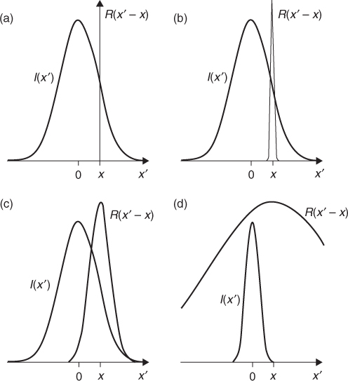
According to the degree of nonlocality, as determined by the relative width of the response function R with respect to the size of the light beam, there are four categories of nonlocality [6, 7]: local, weakly nonlocal, generally nonlocal, and strongly nonlocal. In the limit that the response function is a delta function, ![]() , the NL response is local (Fig. 4.1a). The weak nonlocality applies when the characteristic length of
, the NL response is local (Fig. 4.1a). The weak nonlocality applies when the characteristic length of ![]() is much smaller than the width of the beam (Fig. 4.1b) and the strong nonlocality corresponds to the case of a characteristic length of the NL response much larger than the beam width (Fig. 4.1d). The case of general nonlocality is in between b and d, as shown in Figure 4.1c.
is much smaller than the width of the beam (Fig. 4.1b) and the strong nonlocality corresponds to the case of a characteristic length of the NL response much larger than the beam width (Fig. 4.1d). The case of general nonlocality is in between b and d, as shown in Figure 4.1c.
Figure 4.1 Different degrees of nonlocality, as given by the width of the response function R(x) and the intensity profile I(x). Shown are the (a) local, (b) weakly nonlocal, (c) general, and (d) strongly nonlocal responses.
The general NNSE model naturally arises in NL optics, where it describes the propagation of an electric field envelope in a wave-guiding potential, in the paraxial approximation. The nonlocal index change, induced by the propagating beam, involves some transport-like process, for example, heat transfer in materials with thermal response [29], diffusion of molecules in atomic vapors [30], charge separation in photorefractive crystals [31], or intermolecular links in NLCs [32]. The general NNSE also appears in the description of BECs [33–36], in which case u stands for the collective wave-function and I is the density of atoms in the condensate; V then represents the magnetic trap potential, z is the time, and Equation 4.3 becomes the nonlocal Gross–Pitaevskii (GP) equation [37–39].
In the limit when the response function ![]() is sharply peaked at point
is sharply peaked at point ![]() and much narrower than the intensity distribution
and much narrower than the intensity distribution ![]() , the NL term becomes local, N(I) ≈ I. In NL optics, the model (Eq. 4.3) then becomes the standard NLSE with an external potential, describing local Kerr media. In BECs, it becomes the standard GP equation. In the opposite limit, when the response function is much broader than the intensity distribution, the NL term becomes proportional to the response function, N(I) ≈ PR, with P the beam power. Assuming the intensity distribution peaked at the origin, one can expand the response function about the origin to obtain N(I) ≈ P(R0 + R2r2). In this case, the highly nonlocal NLSE becomes the linear Schrödinger equation with a harmonic potential. A more general treatment in Reference 24, even without the external potential, leads to an NL optical model in which the change in the NL term is proportional to an NL function of the power, ΔN(I) ≈ α2(P)r2. Although linear in u, the model still describes highly NL solitons through the NL dependence of the coefficient α on the beam power P [24]. For this reason, the model is referred to as the strongly nonlocal NLSE. It was used in References 1–3, for instance, to explain the experimental observation of optical spatial solitons in NLCs. In this chapter, we mostly deal with this limit of the general NNSE.
, the NL term becomes local, N(I) ≈ I. In NL optics, the model (Eq. 4.3) then becomes the standard NLSE with an external potential, describing local Kerr media. In BECs, it becomes the standard GP equation. In the opposite limit, when the response function is much broader than the intensity distribution, the NL term becomes proportional to the response function, N(I) ≈ PR, with P the beam power. Assuming the intensity distribution peaked at the origin, one can expand the response function about the origin to obtain N(I) ≈ P(R0 + R2r2). In this case, the highly nonlocal NLSE becomes the linear Schrödinger equation with a harmonic potential. A more general treatment in Reference 24, even without the external potential, leads to an NL optical model in which the change in the NL term is proportional to an NL function of the power, ΔN(I) ≈ α2(P)r2. Although linear in u, the model still describes highly NL solitons through the NL dependence of the coefficient α on the beam power P [24]. For this reason, the model is referred to as the strongly nonlocal NLSE. It was used in References 1–3, for instance, to explain the experimental observation of optical spatial solitons in NLCs. In this chapter, we mostly deal with this limit of the general NNSE.
In the limit of a strongly nonlocal nonlinearity, the evolution of field u in three dimensions is described by the strongly NNSE [10–12, 21, 23, 24]:
where s( > 0) is a parameter proportional to α2(P), containing the effect of beam power. Note that P is constant and equal to the total input power P0. Clearly, the same equation describes the time-dependent linear quantum harmonic oscillator (QHO); hence, in solving Equation 4.5, we also deal with a linear quantum-mechanical problem. Although several solutions to the z-independent QHO in various coordinate systems are known, we look for the self-similar z-dependent solutions of Equation 4.5 in the form of localized D-dimensional spatiotemporal solitons. Such solutions will naturally impose certain conditions on the input parameters and those describing the solutions. It should also be underlined that the beam collapse cannot occur in Equation 4.5, as it is a linear PDE. The second term in Equation 4.5 represents diffraction and the third one originates from the optical nonlinearity. We consider here only the case s > 0.
4.3 Soliton Families in Strongly Nonlocal Nonlinear Media
We discuss several spatial solitons of different dimensions in NN media, such as 1D HG solitons, 2D Laguerre–Gaussian soliton families, 2D self-similar HG solitons, and 2D Whittaker solitons (WS).
4.3.1 One-Dimensional Hermite–Gaussian Spatial Solitons
The interest in self-similar waves in complex NL optical systems has grown greatly in recent years [37–43]. Although self-similar solutions have been extensively studied in several fields, such as plasma physics and nuclear physics [44, 45], in NL optics this interest is relatively young, with only a few optical self-similar phenomena investigated to date [37–39]. Specifically, exact one-dimensional self-similar solitary waves were found in optical fibers in which dispersion, nonlinearity, and gain profile are allowed to change with the propagation distance, but with functionally related forms [40–42].
In the 1D case, Equation 4.5 reduces to
It is easy to obtain the self-similar soliton solution of Equation 4.6:
4.7 
where n = (0, 1, 2, …) is a nonnegative integer, Hn are Hermite polynomials, and w0 denotes the initial width of the beam. The power of the light beam ![]() can be calculated using the orthogonality relations between Hn and is a constant of motion, which does not depend on the degree of the Hermite polynomials. We set it equal to 1. Because Equation 4.6 is linear, NL wave collapse cannot occur. A spatial soliton of this kind can exist only in strongly nonlocal media and is the accessible soliton, with the same form as the standard Hermite modes of 1D QHO.
can be calculated using the orthogonality relations between Hn and is a constant of motion, which does not depend on the degree of the Hermite polynomials. We set it equal to 1. Because Equation 4.6 is linear, NL wave collapse cannot occur. A spatial soliton of this kind can exist only in strongly nonlocal media and is the accessible soliton, with the same form as the standard Hermite modes of 1D QHO.
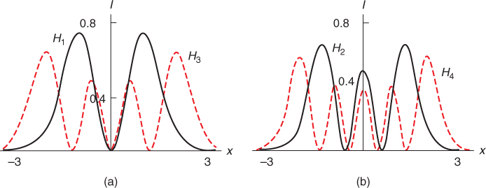
We now illustrate the distributions of amplitude, intensity, and the positions of zeroes and extremal points, where ![]() . Figure 4.2 shows analytical solutions of several low order solitons along the x axis. Figure 4.3 displays the shapes of a few odd and even soliton distributions. When n is even (odd) the optical intensity is nonzero (zero) in the beam center.
. Figure 4.2 shows analytical solutions of several low order solitons along the x axis. Figure 4.3 displays the shapes of a few odd and even soliton distributions. When n is even (odd) the optical intensity is nonzero (zero) in the beam center.
Figure 4.2 Hn solitons, for different n. Here, the parameter n has the values 0–2 from top to bottom.
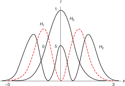
Figure 4.3 Optical field distributions, for different n: (a) odd solitons, for n odd; (b) even solitons, for n even.
4.3.2 Two-Dimensional Laguerre–Gaussian Soliton Families
As mentioned earlier, NLCs are useful dielectrics exhibiting huge optical nonlinearities [46–50], which makes them suitable for investigating NL phenomena with low power lasers and low cost detection equipment. In this section, we study the propagation of a beam in two-dimensional strongly NN media using the wave equation (Eq. 4.5), showing that there is a class of LGnm solitary waves propagating in a self-similar manner. It is found that the predicted self-similar waves can be regarded as a family of spatial solitons.
Exact solutions of Equation 4.5 were obtained in the form of two-dimensional self-similar soliton waves in Reference 17:
where ![]() and
and ![]() are the generalized Laguerre polynomials. Spatial solitons in Equation 4.8 are determined by two parameters, n and m. For a fixed n and various m (or a fixed m and various n), the LGnm solitons share a few characteristics and form a family.
are the generalized Laguerre polynomials. Spatial solitons in Equation 4.8 are determined by two parameters, n and m. For a fixed n and various m (or a fixed m and various n), the LGnm solitons share a few characteristics and form a family.
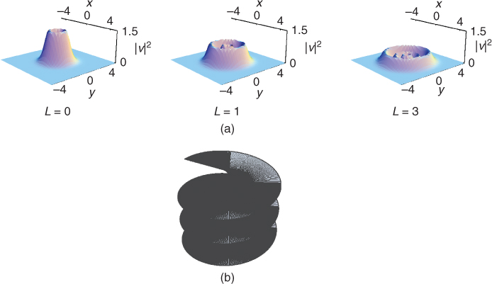
Figure 4.4a shows the radial distribution of low order solitons for m = 0 and various n. There are n zeroes and n + 1 extremal points along the radius. Figure 4.4b and c displays the distribution of the optical field and intensity of LGn0(n = 0, 1, 2, 3) solitons. Their peak intensity is on the propagation axis. Physically, m = 0 indicates that the NL polarization has the symmetry of the electric field due to the strong nonlocality; field and intensity distributions are clearly independent of the azimuthal angle.
Figure 4.4 (a) Amplitudes of radial distributions of LGn0 solitons, corresponding to LG00, LG10, and LG20; (b) optical field distribution of LGn0 solitons with w0 = 1 and P0 = 1; (c) intensity distributions viewed from above of LGn0 solitons with w0 = 1 and P0 = 1.
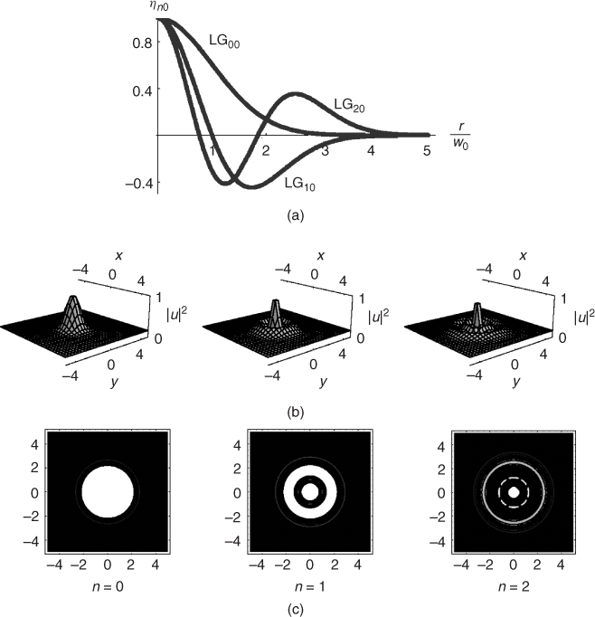
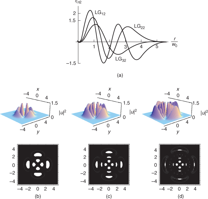
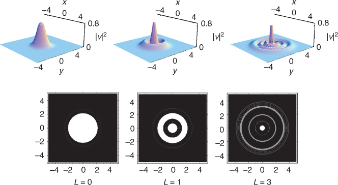
Figure 4.5 illustrates some properties of LGn2 solitons for m > 0 and q = 0. The amplitude ηn2 has n + 1 zeroes and n + 1 extremal points along the radius. Moreover, there are 2m zeroes and 2m extremal points along the azimuth direction. In contrast to the case m = 0, the optical intensity is zero at the center. As seen from Figures 4.4a and 4.5a, LGnm solitons decay fast in transverse space. This stems from nonlocality, as the NL polarization in a small volume of radius r0 (r0 ![]() any wavelength involved) depends not only on the electric field within this volume but also on its value outside and around it within the nonlocal range.
any wavelength involved) depends not only on the electric field within this volume but also on its value outside and around it within the nonlocal range.
Figure 4.5 (a) Amplitude distributions of LGn2 solitons. (b–d) Optical field and intensity distributions viewed from above of LG12, LG22, and LG32 solitons with w0 = 1 and P0 = 1.
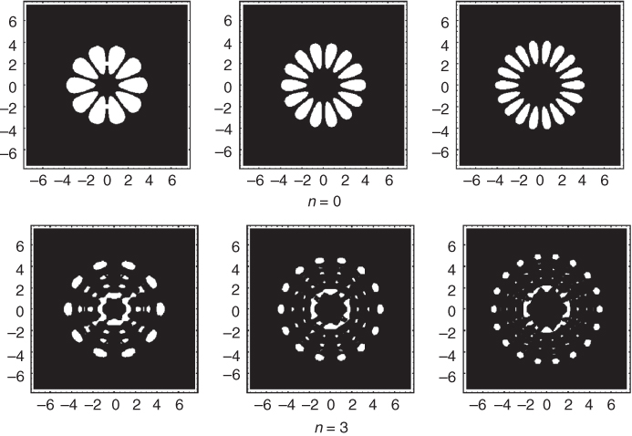
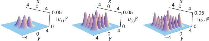
We now discuss multipole solitons (q = 0) when n = 0, 3 for various m. For the LG00 soliton, the amplitude η00 has no zeros along the radial direction. Other solitons have one and more zeroes (Figure 4.4a). Figure 4.6 shows intensity distributions for various m when n = 0, 3. The distributions change regularly along the azimuth; when m is large enough, the beam forms a ring (necklace soliton) [51]. In strongly NN media, the refractive index is determined by the intensity distribution over the entire transverse plane and the nonlocality can lead to a refractive index increase in the region r0 (r0 ![]() any wavelength involved), supporting multipole solitons. Note that the nonlocal response function is much wider than the beam itself [52–55], thus the width of the index distribution greatly exceeds the size of an individual spot [56].
any wavelength involved), supporting multipole solitons. Note that the nonlocal response function is much wider than the beam itself [52–55], thus the width of the index distribution greatly exceeds the size of an individual spot [56].
Figure 4.6 LGnm solitons when n and m are varied. Upper row n = 0, lower row n = 3; m = 1, 2, 3 from left to right.
4.3.3 Accessible Solitons in the General Model of Beam Propagation in NLC
In this section, we present the self-similar method for the general (2 + 1)D model of light propagation in NLC, previously introduced in Equations 4.1 and 4.2 but conveniently simplified with reference to the NLC cell geometry reported in References 48 and 57. The field envelope is polarized along x and propagates along z. The evolution of the paraxial envelope E and the tilt angle θ are described by Peccianti et al. [47, 48, 57]:
where ![]() is the dielectric anisotropy of the medium and k ≈ k0
is the dielectric anisotropy of the medium and k ≈ k0 ![]() . Steady state is assumed. The parameters k and k0 are the wave numbers in NLC and in vacuum, respectively; ε 0 is the vacuum permittivity; θ0 is the tilt of NLC molecules in the absence of light (as mentioned, the value θ0 = π/4 corresponds to the minimum Frédericksz threshold); and K is the average Frank elastic constant. We work in cylindrical coordinates, φ is the azimuthal angle and
. Steady state is assumed. The parameters k and k0 are the wave numbers in NLC and in vacuum, respectively; ε 0 is the vacuum permittivity; θ0 is the tilt of NLC molecules in the absence of light (as mentioned, the value θ0 = π/4 corresponds to the minimum Frédericksz threshold); and K is the average Frank elastic constant. We work in cylindrical coordinates, φ is the azimuthal angle and ![]() is the radial distance.
is the radial distance.
For a finite radial distance from the beam axis (r = 0), the dipole-induced perturbation is much wider than the beam itself [48], with ![]() . Here, β
. Here, β ![]() is a small optically induced correction to the orientation angle of the director; hence, β0 corresponds to the peak in the director angle distribution and θ0 to the background value. After the normalization V = E/E0, with E0 = E(r = 0, z = 0), in the highly nonlocal limit, we can reduce the two coupled Equations 4.9 and 4.10 to one:
is a small optically induced correction to the orientation angle of the director; hence, β0 corresponds to the peak in the director angle distribution and θ0 to the background value. After the normalization V = E/E0, with E0 = E(r = 0, z = 0), in the highly nonlocal limit, we can reduce the two coupled Equations 4.9 and 4.10 to one:
where ![]() ,
, ![]() , and
, and ![]() . The novelty here is that the parabolic term has acquired z dependence, stemming from the on-axis beam intensity. We have found an approximate analytical self-similar solution of Equation 4.11:
. The novelty here is that the parabolic term has acquired z dependence, stemming from the on-axis beam intensity. We have found an approximate analytical self-similar solution of Equation 4.11:
4.12 
where α is the normalization constant and P0 is the beam power. w(z), a(z), and c(z) are determined by Equations 4.20 and 4.21 and other parameters must satisfy the constraints of Equation 4.17. W satisfies
Equation 4.13 is the well-known Whittaker differential equation, with solutions known as Whittaker functions (sometimes also called the parabolic cylinder functions) [58]:
4.14 
where the real part is Re[l − l/2 + m/2] ≥ 0, l − l/2 + m/2 is not an integer, l is a real number, and Γ is the Gamma function. The parameters have to satisfy the following equations:
4.16 ![]()
Taking ![]() and
and ![]() , after integrating Equation 4.15 one gets
, after integrating Equation 4.15 one gets
where η = w/w0 and ![]() . As
. As ![]() , we have lnη2 ≈ η2 − 1. Integrating Equation 4.18, we find
, we have lnη2 ≈ η2 − 1. Integrating Equation 4.18, we find
4.19 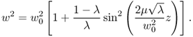
Thus, the phase offset and the wave front curvature of the beam can be obtained:
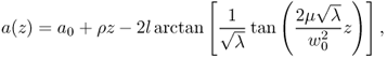
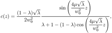
where ![]() .
.
When λ = 1, the beam size is independent on the propagation distance and becomes a shape-preserving accessible soliton [24]. Its phase offset, width, and the wave front curvature are given by ![]() , w(z) = w0, and c(z) = 0, respectively. Thus, the approximate self-similar soliton solution of Equation 4.11 can be cast as
, w(z) = w0, and c(z) = 0, respectively. Thus, the approximate self-similar soliton solution of Equation 4.11 can be cast as
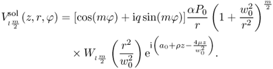
The parameters of this solution must satisfy the important constraint (Eq. 4.17). It is interesting to note that a spatial soliton of any constant width can propagate in NLC as long as ![]() (namely, λ = 1). However, this condition is not usually experimentally met and solitons typically breathe. It should also be noted that χ is a parameter determined by the specific NLC and the initial beam width. We find that the 2D spatial solitons of Equation 4.22 are defined by the parameters (l, m) and q. In what follows, we describe various structures by studying the field distributions, the intensities of radial distributions, the positions of zeroes, and the extremal points of solutions. We choose the initial conditions w0 = 1, P0 = 1.
(namely, λ = 1). However, this condition is not usually experimentally met and solitons typically breathe. It should also be noted that χ is a parameter determined by the specific NLC and the initial beam width. We find that the 2D spatial solitons of Equation 4.22 are defined by the parameters (l, m) and q. In what follows, we describe various structures by studying the field distributions, the intensities of radial distributions, the positions of zeroes, and the extremal points of solutions. We choose the initial conditions w0 = 1, P0 = 1.
When m is an integer, introducing the relation ![]() , from Equation 4.13, we obtain the generalized Laguerre differential equation:
, from Equation 4.13, we obtain the generalized Laguerre differential equation:
4.23 ![]()
Its solutions are the generalized Laguerre polynomials ![]() . Therefore, the solution of Equation 4.11 may also be expressed as
. Therefore, the solution of Equation 4.11 may also be expressed as
where 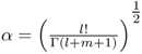 .
.
4.3.3.1 Gaussian Solitons (m = 0)
When m = 0, the relation (Eq. 4.17) is naturally satisfied, and Equation 4.24 can be simplified to ![]() . Figure 4.7 shows analytical solutions of Gaussian solitons for various l. There are l zero points (dark rings) and l + 1 extreme points (bright rings) along the radial direction for Ll0 solitons. The peak optical intensity is at the origin.
. Figure 4.7 shows analytical solutions of Gaussian solitons for various l. There are l zero points (dark rings) and l + 1 extreme points (bright rings) along the radial direction for Ll0 solitons. The peak optical intensity is at the origin.
Figure 4.7 Gaussian solitons, for different l, when m = 0. Top row is the optical field distributions and the bottom row is the view from above. The parameter l is l = 0, 1, 3 from left to right.
4.3.3.2 Radially Symmetric Solitons (q = 1, m Positive Integer)
In the limit q = 1 for m( > 0), a nonnegative integer, Equation 4.17 is automatically satisfied. Equation 4.24 generates radially symmetric solitons, which can be expressed as ![]() . Figure 4.8 illustrates some features of these solitons. For equal l, the larger the m, the faster the field decay. The intensity is zero at (x, y) = (0, 0).
. Figure 4.8 illustrates some features of these solitons. For equal l, the larger the m, the faster the field decay. The intensity is zero at (x, y) = (0, 0).
Figure 4.8 Radially symmetric solitons for l = 1 and q = 1. Top row is the optical field distribution and the bottom row is the view from above.
4.3.3.3 Multipole Solitons (l Nonnegative Integer,  , q = 0)
In the limit q = 0, we must take ![]() , in order to satisfy Equation 4.17. This case is similar to the previous one. In particular, when |V(0, z)|2 = const. Equation 4.11 reduces to the Snyder–Mitchell model of accessible solitons [24]. From Equation 4.24, we obtain
, in order to satisfy Equation 4.17. This case is similar to the previous one. In particular, when |V(0, z)|2 = const. Equation 4.11 reduces to the Snyder–Mitchell model of accessible solitons [24]. From Equation 4.24, we obtain ![]() , which forms multipole solitons. These multipole solutions contain single-layer necklace solitons (l = 0 but
, which forms multipole solitons. These multipole solutions contain single-layer necklace solitons (l = 0 but ![]() ) and multilayer necklace solitons (l is a positive integer but
) and multilayer necklace solitons (l is a positive integer but ![]() ). Figure 4.9 shows examples of multipole solitons.
). Figure 4.9 shows examples of multipole solitons.
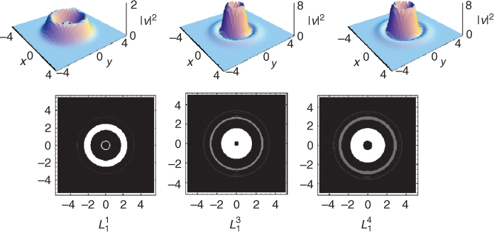
Figure 4.9 Multipole solitons. (a) l = 0, for different m; (b) l = 2, for different m.
Interesting structures can be seen for different multipole solitons. The larger the parameter m, the larger the necklace radius. The distributions change regularly with the azimuth. For a large enough m, the bright spots form a ring. These multipole solitons contain 2m spots and l + 1 ring layers.
4.3.3.4 Fractional Solitons (m Noninteger) and Soliton Vortices
When q = 1 and m is a noninteger, interesting structures are formed. Figure 4.10 shows field distributions for m = 1/2 and various l. As apparent from Equations 4.20 and 4.21, at the point of phase singularity the phase is undefined and the intensity vanishes, thus yielding a vortex. The soliton wave rotates around the vortex core in a given direction (the sign of m defines the rotation direction), with infinite angular velocity at (x, y) = (0, 0). An interesting feature is the clockwise rotation of the vortex core with the simultaneous relaxation to the radially symmetric profile.
Figure 4.10 (a) Field intensity of fractional solitons, showing single, double, and triple summits for m = 0.5 and different l; (b) Optical beam helical wave front.
Analytical solutions of Equation 4.11 were obtained exactly and novel solitons found in NLC, including Gaussian solitons, radially symmetric solitons, multipole necklace solitons, and vortex solitons. These solitons are solutions to Equation 4.11, the strongly nonlocal approximation to the original model of Equations 4.9 and 4.10. It is plausible, although not yet proven, that these solitons appear in the full model and are stable or quasi-stable for prolonged propagation distances.
4.3.4 Two-Dimensional Self-Similar Hermite–Gaussian Spatial Solitons
In this section, starting from the Snyder–Mitchell model, we construct higher order spatial solitons propagating in a self-similar manner in NN media. We look for these solutions in Cartesian coordinates.
In the limit of a strong nonlocal nonlinearity and in Cartesian coordinates, the wave equation in 2D NN media is the general NNSE [10–12, 24]:
This equation is equivalent to the 2D QHO, with several known solutions in the time (or z)-independent case. They range from 1D to 4D (for hydrogen atom) and even higher (in quantum field theories). We have obtained the z-dependent solution to Equation 4.25, using the self-similar method [59]. We provide here the soliton solution:
4.26 ![]()
where ![]() . The solution is expressed in terms of 2D HG functions, as one would expect from a QHO problem. The z dependence is explicitly present in the beam width and the wave front curvature of the general solution [59]. Here, for a soliton solution, the phase offset is given by
. The solution is expressed in terms of 2D HG functions, as one would expect from a QHO problem. The z dependence is explicitly present in the beam width and the wave front curvature of the general solution [59]. Here, for a soliton solution, the phase offset is given by ![]() , the curvature is zero, and w = w0.
, the curvature is zero, and w = w0.
Figure 4.11a illustrates a few properties of solutions for arbitrary n and m. The (n + 1) × (m + 1) extremal points are arranged in a rectangular matrix. The farther the spot is from the center of the transverse axes, the greater is the intensity. The intensity is zero at the beam center when n (or m) is even; conversely, when n is odd the intensity is the smallest extremum at the center. When ![]() , the soliton forms a square matrix of spots. Figure 4.12 displays a few soliton square distributions.
, the soliton forms a square matrix of spots. Figure 4.12 displays a few soliton square distributions.
Figure 4.11 Optical field distributions of HG solitons, for different parameters. (a) n = 1, m = 1, 3, 5. (b) n = 1, m = 2, 4, 6.
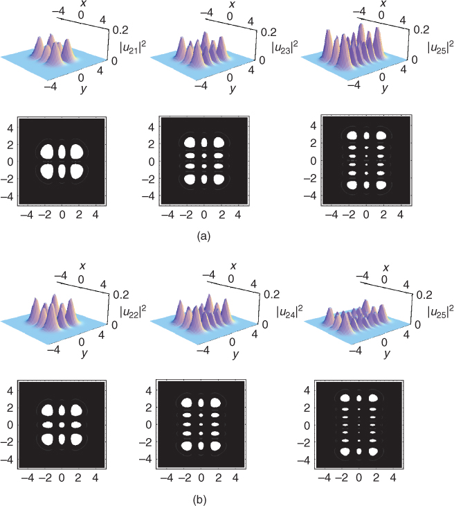
Figure 4.12 Typical square matrix HG solitons. The parameters are n = m = 2; n = m = 3; and n = m = 4 from left to right, respectively.
In summary, self-similar waves of HG spatial solitons in strongly NN media were studied analytically. Exact solutions were obtained in the form of HGmn functions with interesting properties, including shape-preserving as well as breathing beams.
4.3.5 Two-Dimensional Whittaker Solitons
In this section, starting from a set of linear Whittaker modes, we construct higher order spatial solitons in NN media in the form of WS. We display different possible WS families: Gaussian solitons, vortex-ring solitons, half-moon solitons, and symmetric and asymmetric single- and multilayer necklace solitons. We find that some classes of WS display well-defined symmetry and give rise to stable solitons, whereas others exhibit an unstable behavior typical of multidimensional soliton clusters [54], although their stability may be improved. Although our conclusions on enhanced stability are based on numerical studies, definitive answers must await a more thorough analysis.
We consider the propagation of beams in an NN medium in the paraxial approximation, described by the generalized NNSE; see Equations 4.3 and 4.4 for the scalar electric field envelope ![]() :
:
4.28 ![]()
As mentioned earlier, in the limit that the response function is a delta function ![]() , the nonlinearity becomes proportional to the intensity,
, the nonlinearity becomes proportional to the intensity, ![]() and we recover the local limit of NNSE, that is, the NLSE. In the opposite limit, when the response function is much broader than the intensity distribution, the nonlinearity becomes proportional to the response function,
and we recover the local limit of NNSE, that is, the NLSE. In the opposite limit, when the response function is much broader than the intensity distribution, the nonlinearity becomes proportional to the response function, ![]() with P the beam power. In this strongly nonlocal limit, the NNSE becomes the linear SE with a given potential. In this case, the NNSE becomes the SE for the QHO, supporting accessible solitons [24]. We have shown that the strongly nonlocal NLSE also possesses exact self-similar 2D soliton solutions [21]:
with P the beam power. In this strongly nonlocal limit, the NNSE becomes the linear SE with a given potential. In this case, the NNSE becomes the SE for the QHO, supporting accessible solitons [24]. We have shown that the strongly nonlocal NLSE also possesses exact self-similar 2D soliton solutions [21]:
4.29 ![]()
where ![]() ,
, ![]() ,
, ![]() , and
, and ![]() . The parameter m is a real constant called the vorticity or topological charge [12, 60], n is a nonnegative integer, and w0 is the initial beam width. The parameter
. The parameter m is a real constant called the vorticity or topological charge [12, 60], n is a nonnegative integer, and w0 is the initial beam width. The parameter ![]() determines the modulation depth of the beam intensity. Wnm(θ) are the Whittaker functions, defined as [61]
determines the modulation depth of the beam intensity. Wnm(θ) are the Whittaker functions, defined as [61]
4.30 ![]()
with Γ the Gamma function. In the argument of the Gamma function, we assume ![]() . Note the differences between this solution, presented in terms of Whittaker functions, and the one presented in the previous section, where Whittaker differential equations and functions also appeared. Being solutions to the linear SE, the self-similar WS functions unm(z, r, φ) are stable, without beam collapse. In analogy with these solutions, we look for WS solutions of Equation 4.27 with enhanced stability, in the form u(z, r, φ) = rmΦ(φ)V(z, r), where Φ = cos(mφ) + iqsin(mφ). Such a choice in the azimuthal function dependence allows for more freedom in the characterization of possible solitons. In this case, Equation 4.27 acquires the form
. Note the differences between this solution, presented in terms of Whittaker functions, and the one presented in the previous section, where Whittaker differential equations and functions also appeared. Being solutions to the linear SE, the self-similar WS functions unm(z, r, φ) are stable, without beam collapse. In analogy with these solutions, we look for WS solutions of Equation 4.27 with enhanced stability, in the form u(z, r, φ) = rmΦ(φ)V(z, r), where Φ = cos(mφ) + iqsin(mφ). Such a choice in the azimuthal function dependence allows for more freedom in the characterization of possible solitons. In this case, Equation 4.27 acquires the form
At this point, one has to specify the response function; different possibilities exist and depend on the physical situation [62]. As long as the response function is real, symmetric, positive, and monotonically decaying, the properties of the solutions do not depend much on the shape of the response function [60]. We therefore choose the Gaussian ![]() for simplicity [60, 62], and also because it offers stable solutions [63, 64]. The Gaussian width σ controls the nonlocality: when
for simplicity [60, 62], and also because it offers stable solutions [63, 64]. The Gaussian width σ controls the nonlocality: when ![]() , we retrieve the local Kerr model. Here, we take σ = 1 and P = 1. This does not imply that we are in the strongly nonlocal regime, because this also depends on the width and the height of the expected solution V; however, by a judicious choice of the parameters and an appropriate numerical procedure one can find solutions that propagate quasi-stably over prolonged distances. For larger values of σ and P, that is, by moving deeper into the nonlocal regime, the stability of the numerical solutions improves.
, we retrieve the local Kerr model. Here, we take σ = 1 and P = 1. This does not imply that we are in the strongly nonlocal regime, because this also depends on the width and the height of the expected solution V; however, by a judicious choice of the parameters and an appropriate numerical procedure one can find solutions that propagate quasi-stably over prolonged distances. For larger values of σ and P, that is, by moving deeper into the nonlocal regime, the stability of the numerical solutions improves.
To find stationary soliton solutions of Equation 4.31, we resort to a variational procedure described in detail in Reference 65. By choosing initial conditions consistent with the linear WS solutions
4.32 ![]()
and also for w0 = 1 and a1 = 0, we obtain the propagating WS solutions of Equation 4.31. Such a choice of the initial field allows having the propagating fields with fractional topological charges m, provided the parameter q is chosen accordingly [66]. Figures 4.13 to 4.16 show contour plots of the real field u distributions in 2D, for some specific values of the above parameters. We also compare the results for σ = 1 and P = 1 with the ones for σ = 100 and P = 100, to ascertain the improved stability.
Figure 4.13 Gaussian WS family (m = 0). (a) Dependence along the radial direction, showing the positions of zeroes (unm = 0) and extremal points (![]() ) for three values of n = 1, 3, 5, from left to right. The field distributions in (b) and (c) are at different propagation distances z = 10, 100 from top to bottom. In (b) σ = 1, P = 1; in (c) σ = 100, P = 100.
) for three values of n = 1, 3, 5, from left to right. The field distributions in (b) and (c) are at different propagation distances z = 10, 100 from top to bottom. In (b) σ = 1, P = 1; in (c) σ = 100, P = 100.
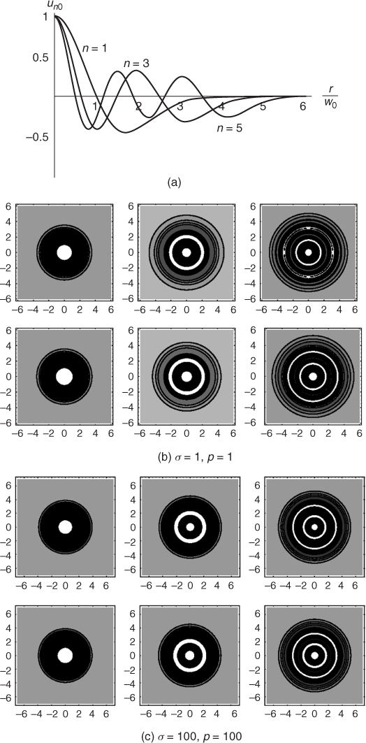
Figure 4.14 (a) Vortex-ring WS family without the complex function Φ(φ) (layout as shown in Figure 4.13). Here m = 1, q = 1, and n = 1, 3, 5. The two rows in (b) and (c) present the field distributions at distances z = 10, 100, respectively. In (b) σ = 1, P = 1 and in (c) σ = 100, P = 100.
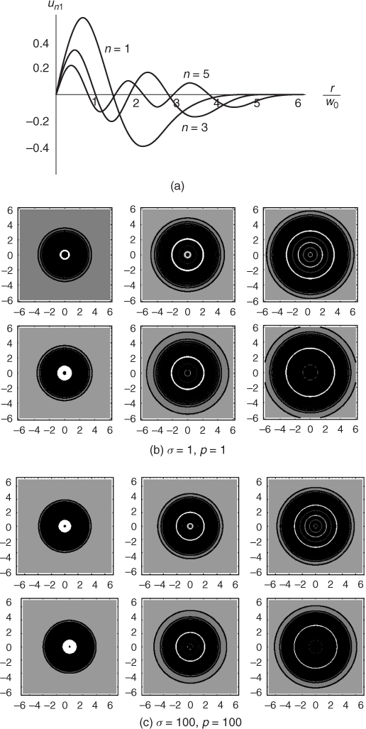
Figure 4.15 Modulational instability in the half-moon soliton family, for m = 1/2 and q = 0. (a) Field distribution in z = 0. (b and c) Top views at propagation distances z = 10, 100, from top to bottom. In (b) σ = 1, P = 1 and in (c) σ = 100, P = 100, respectively. n = 1, 3, 5, from left to right in each graph.
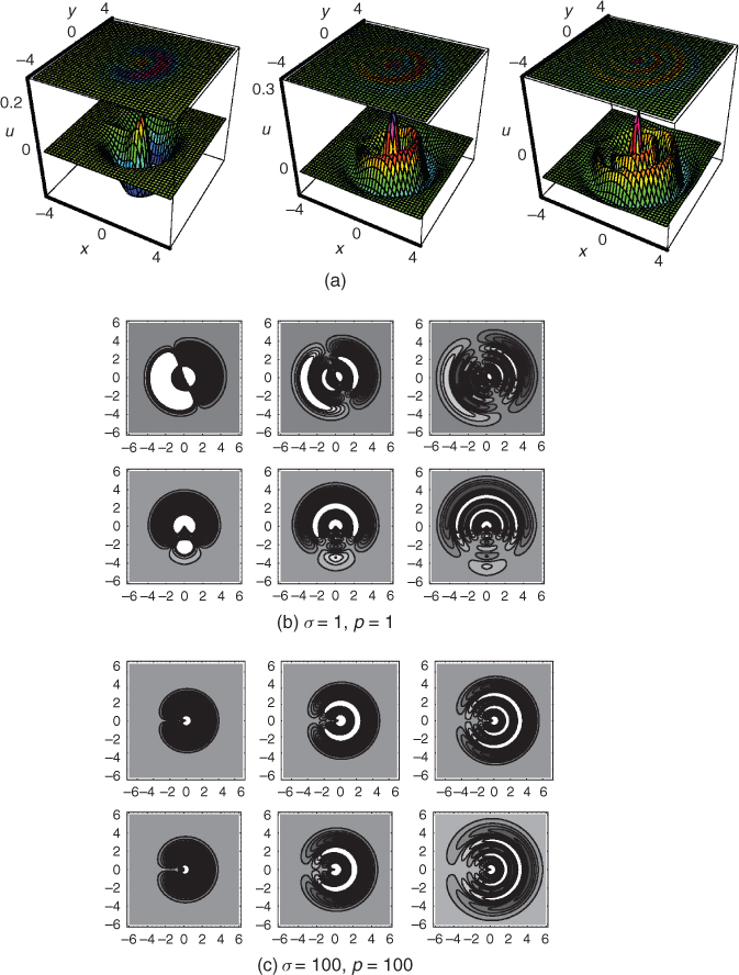
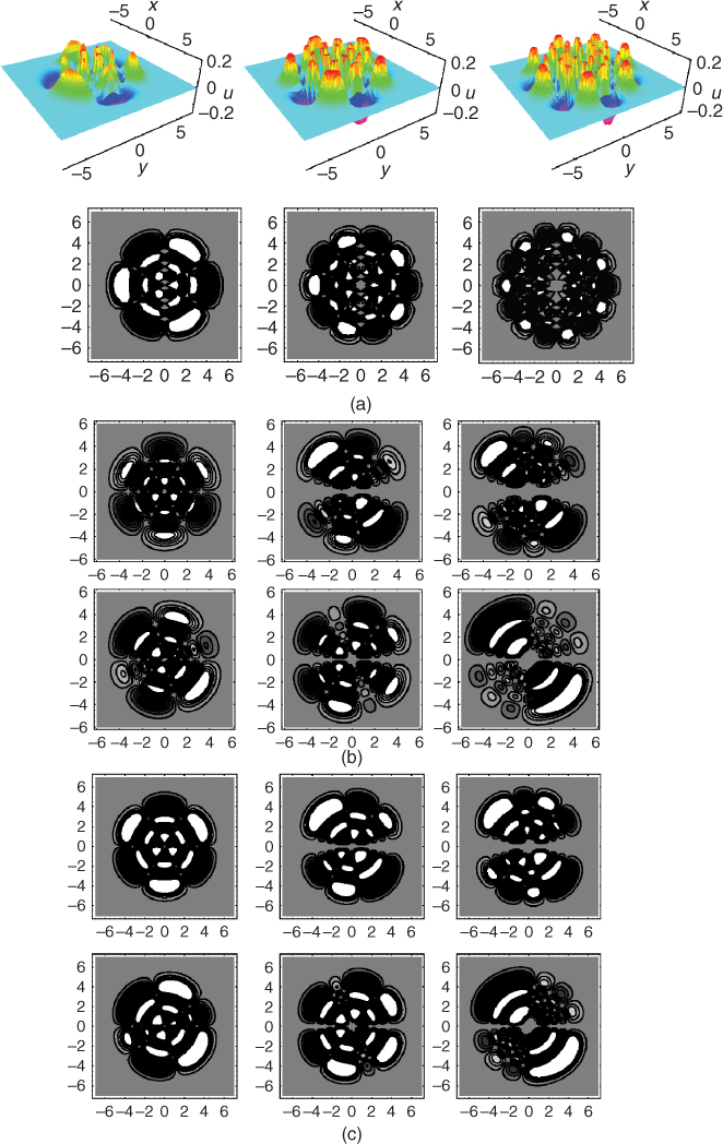
Figure 4.16 Symmetric multipole soliton distributions, for n = 3 and q = 0. Layout is similar to that shown in Figure 4.15. (a) Field distributions at z = 0. (b and c) Views from above, for z = 10, 100 from top to bottom. In (b) σ = 1, P = 1 and in (c) σ = 100, P = 100, respectively. In all the graphs m = 3, 5, 7 from left to right.
4.3.5.1 Gaussian and Vortex-Ring Solitons
Figure 4.13 presents the stable Gaussian WS family (m = 0) and Figure 4.13 the stable vortex-ring soliton family (q = 1, ![]() ) for various n. Figure 4.13a shows the radial dependence, including the positions of zeroes and extremal points of Gaussian WS. Figure 4.13a displays the field distribution at z = 0. The two rows in Figure 4.13b and c plot field distributions taken at propagation distances z = 10, 100 (units of diffraction lengths) for σ = 1, P = 1 and for σ = 100, P = 100, respectively. The nearly constant distributions versus z indicate stable propagation. There are n zeroes and n + 1 extrema along the radius. The bright spots or rings in Figure 4.13b and c represent the positive extrema, the dark rings represent the negative extrema. The maximum field is located at the origin.
) for various n. Figure 4.13a shows the radial dependence, including the positions of zeroes and extremal points of Gaussian WS. Figure 4.13a displays the field distribution at z = 0. The two rows in Figure 4.13b and c plot field distributions taken at propagation distances z = 10, 100 (units of diffraction lengths) for σ = 1, P = 1 and for σ = 100, P = 100, respectively. The nearly constant distributions versus z indicate stable propagation. There are n zeroes and n + 1 extrema along the radius. The bright spots or rings in Figure 4.13b and c represent the positive extrema, the dark rings represent the negative extrema. The maximum field is located at the origin.
The layout of Figure 4.14 is similar to that shown in Figure 4.13. The field u of the vortex-ring WS is shown excluding the azimuthal complex function Φ(ϕ). Similarly, there are n + 1 zeroes and n + 1 extrema along the radius; the bright ring represents the positive extrema and the dark spots and rings represent the negative extrema. At the origin, where the topological defect is located, the field is zero. The fields of these two classes of solitons are radially symmetric and decaying. We find that 2D Gaussian WS and vortex-ring WS can propagate stably in NN media in the highly nonlocal limit.
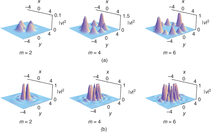
4.3.5.2 Half-Moon Solitons
When ![]() but q = 0 ( − 1/4 ≤ m < 1), we obtain the asymmetric half-moon WS family. For the parameters considered here, half-moon solitons display modulational instability. Figure 4.15 shows the shapes of typical half-moon solitons for q = 0, m = 1/2 and for various n. Clearly, the half-moon soliton is stratified in a circular arrangement, because of the cosine azimuthal dependence. Bright (dark) regions represent a positive (negative) field with
but q = 0 ( − 1/4 ≤ m < 1), we obtain the asymmetric half-moon WS family. For the parameters considered here, half-moon solitons display modulational instability. Figure 4.15 shows the shapes of typical half-moon solitons for q = 0, m = 1/2 and for various n. Clearly, the half-moon soliton is stratified in a circular arrangement, because of the cosine azimuthal dependence. Bright (dark) regions represent a positive (negative) field with ![]()
![]() . The uniform gray corresponds to zero and the innermost layer is a bright spot. The half-moon soliton alternates bright and dark regions from inside to outside along every radial direction, except along the negative real axis, where it is null. The number of layers depends on n and there are n + 1 layers. At the initial stage (z = 0), the solitons display the half-moon shape [67], as the numerical solutions stem from the modulated WS modes. Along propagation (Fig. 4.15b) we observe that, at z = 10, the WS break up into two out-of-phase portions, each similar to the initial half-moon. At z = 100, these distributions become two irregular half-moon solitons. The larger the parameter n, the larger the half-moon WS deformation with propagation distance, indicating strong modulational instabilities. However, if larger values of σ and P are chosen, for example, σ = 100, P = 100, the propagation of half-moon solitons becomes more stable, although with slight diffraction, as shown in Figure 4.15c.
. The uniform gray corresponds to zero and the innermost layer is a bright spot. The half-moon soliton alternates bright and dark regions from inside to outside along every radial direction, except along the negative real axis, where it is null. The number of layers depends on n and there are n + 1 layers. At the initial stage (z = 0), the solitons display the half-moon shape [67], as the numerical solutions stem from the modulated WS modes. Along propagation (Fig. 4.15b) we observe that, at z = 10, the WS break up into two out-of-phase portions, each similar to the initial half-moon. At z = 100, these distributions become two irregular half-moon solitons. The larger the parameter n, the larger the half-moon WS deformation with propagation distance, indicating strong modulational instabilities. However, if larger values of σ and P are chosen, for example, σ = 100, P = 100, the propagation of half-moon solitons becomes more stable, although with slight diffraction, as shown in Figure 4.15c.
4.3.5.3 Symmetric Multipole Solitons
When m > 0 is an integer and q = 0, we obtain symmetric multipole solitons, including symmetric single- and multilayer necklace solitons. Once again, their initial distributions stem from the linear WS modes at z = 0. In propagation, they experience strong modulational instabilities. Figure 4.16 shows some examples. These soliton families have adjacent alternating bright and dark regions along the azimuth. For n = 0, the field at z = 0 along the radius has only one layer and the WS form symmetric single-layer necklace solitons. Increasing the propagation distance, these WS families become strongly asymmetric. The number of bright (or dark) spots decreases and the adjacent bright (or dark) spots overlap and merge along the azimuth, as at z = 100.
For n > 0, we observe the symmetric multilayer necklace WS. At z = 0 they form adjacent alternating bright and dark regions along the radial direction, as well. There are n + 1 layers and the maximum field is located at the outside layer along the radius. As shown in Figure 4.16b and c, by increasing the propagation distance the symmetric multipole WS families experience symmetry-breaking instability and merging phenomena for larger m. For m = 7, for example, in the bottom rows, the number of bright/dark regions and their contrast reduce with propagation. They maintain n = 1 layers along the radius but become asymmetric multipole solitons, with a decreasing number of bright and dark regions. However, the stability of symmetric necklace WS greatly improves; that is, they propagate stably and without merging for longer distances, provided larger σ and P are selected. This is clearly seen in Figure 4.16c.
4.3.5.4 Asymmetric Multipole Solitons
In the limit q = 0 and for m > 1, a rational number, we observe asymmetric multipole soliton families. For m we pick half-integer values, because theoretical studies [66] suggest an interesting dynamical behavior there. These asymmetric multipole WS contain asymmetric single- and multilayer necklace solitons (see also Reference 15).
4.4 Conclusions
Spatial solitons in NLCs have stimulated broad interest. Soliton families in strongly NN media have also attracted attention in applied sciences. During the last few years, not only the existence of nonlocal spatial solitons was experimentally demonstrated but also various desirable features were identified and mathematically modeled. Spatial solitons involve a large number of problems, including the exact analytical solutions of the NLSE in various forms and dimensions. The corresponding theories have produced good agreement with experiments and displayed the potential of spatial solitons in applications. We expect the research on soliton families to develop further theoretically, experimentally, and in the quest for actual implementations.
In conclusion, in this chapter, we have provided a mathematical framework for the theoretical understanding of NL nonlocal localization phenomena in NLCs. We have introduced two techniques: the first uses the self-similar method, which is effective when considering soliton symmetries; the second is based on numerical methods. Starting from the general NLSE, in the limit of strong nonlocal nonlinearity, and employing self-similar approach, the evolution equations have been simplified to the highly nonlocal NLSE, yielding exact accessible soliton solutions in one and two dimensions. Numerical methods were employed to solve the general NLS equation, and the exact solutions were used as initial conditions. The numerics were based on the split-step Fourier method, also known as the beam-propagation method. We have further discussed the stability of soliton solutions by comparing analytical and numerical results. We have made an attempt to summarize the most relevant mathematical aspects concerning nonlocal spatial soliton families in NLCs; however, owing to the remarkable recent growth of activities in the field, a few important contributions could not be covered here. Some of those are addressed in other chapters of this book.
Acknowledgments
This work was funded by several agencies, including the National Science Foundation of Guangdong Province, under Grant No. 1015283001000000 (China), the Science Research Foundation of Shunde Polytechnic (China), and the Qatar National Research Foundation through the project NPRP 09-462-1-074 (Qatar).
1. G. Assanto and M. Karpierz. Nematicons: Self-localised beams in nematic liquid crystals. Liq. Cryst., 36(10):1161–1172, 2009.
2. G. Assanto, A. Fratalocchi, and M. Peccianti. Spatial solitons in nematic liquid crystals: from bulk to discrete. Opt. Express, 15(8):5248–5259, 2007.
3. G. Assanto, M. Peccianti, and C. Conti. Nematicons: Optical spatial solitons in nematic liquid crystals. Opt. Photon. News, 14(2):44–48, 2003.
4. C. Rotschild, O. Cohen, O. Manela, M. Segev, and T. Carmon. Solitons in nonlinear media with an infinite range of nonlocality: First observation of coherent elliptic solitons and of vortex-ring solitons. Phys. Rev. Lett., 95:213904, 2005.
5. W. Krolikowski and O. Bang. Solitons in nonlocal nonlinear media: Exact solutions. Phys. Rev. E, 63:016610, 2001.
6. W. Krolikowski, O. Bang, J. J. Rasmussen, and J. Wyller. Modulational instability in nonlocal nonlinear Kerr media. Phys. Rev. E, 64:016612, 2001.
7. S. K. Srivatsa and G. S. Ranganath. New nonlinear optical processes in liquid crystals. Opt. Commun., 180:346–359, 2000.
8. J. Henninot, M. Debailleul, F. Derrien, G. Abbate, and M. Warenghem. (2D + 1) Spatial optical solitons in dye doped liquid crystals. Synt. Met., 124:9–13, 2001.
9. D. Deng, X. Zhao, Q. Guo, and S. Lan. Hermite-Gaussian breathers and solitons in strongly nonlocal nonlinear media. J. Opt. Soc. Am. B, 24:2537–2544, 2007.
10. E. A Sziklas and A. E. Siegman. Mode calculations in unstable resonators with flowing saturable gain. 2: Fast Fourier transform method. Appl. Opt., 14:1874–1889, 1975.
11. B. Fornberg and G. B. Whitham. A numerical and theoretical study of certain nonlinear wave phenomena. Philos. Trans. R. Soc. London, Ser. A, 289:373–403, 1978.
12. W. P. Zhong and L. Yi. Two-dimensional Laguerre-Gaussian soliton family in strongly nonlocal nonlinear media. Phys. Rev. A, 75:061801, 2007.
13. M. Solja![]() i
i![]() and M. Segev. Integer and fractional angular momentum borne on self-trapped necklace-ring beams. Phys. Rev. Lett., 86:420–423, 2001.
and M. Segev. Integer and fractional angular momentum borne on self-trapped necklace-ring beams. Phys. Rev. Lett., 86:420–423, 2001.
14. A. S. Desyatnikov and Y. S. Kivshar. Rotating optical soliton clusters. Phys. Rev. Lett., 88:053901, 2002.
15. W. P. Zhong, M. Beli![]() , R. H. Xie, and G. Chen. Two-dimensional Whittaker solitons in nonlocal nonlinear media. Phys. Rev. A, 78:013826, 2008.
, R. H. Xie, and G. Chen. Two-dimensional Whittaker solitons in nonlocal nonlinear media. Phys. Rev. A, 78:013826, 2008.
16. W. P. Zhong, M. Beli![]() , R. H. Xie, and T. W Huang. Three-dimensional Bessel light bullets in self-focusing Kerr media. Phys. Rev. A., 82:033834, 2010.
, R. H. Xie, and T. W Huang. Three-dimensional Bessel light bullets in self-focusing Kerr media. Phys. Rev. A., 82:033834, 2010.
17. W. P. Zhong, Z. P. Yang, R. H. Xie, M. Beli![]() , and G. Chen. Two-dimensional spatial solitons in nematic liquid crystals. Commun. Theor. Phys., 51:324–330, 2009.
, and G. Chen. Two-dimensional spatial solitons in nematic liquid crystals. Commun. Theor. Phys., 51:324–330, 2009.
18. M. Beli![]() and W. P. Zhong. Two-dimensional spatial solitons in highly nonlocal nonlinear media. Eur. J. Phys. D, 53:97–106, 2009.
and W. P. Zhong. Two-dimensional spatial solitons in highly nonlocal nonlinear media. Eur. J. Phys. D, 53:97–106, 2009.
19. B. A. Malomed, D. Mihalache, F. Wise, and L. Torner. Spatiotemporal optical solitons. J. Opt. B: Quantum Semiclass. Opt., 7:53–72, 2005.
20. B. B. Baizakov, B. A. Malomed, and M. Salerno. Multidimensional solitons in periodic potentials. Europhys. Lett., 63:642–648, 2003.
21. W. P. Zhong, L. Yi, R. H. Xie, M. Beli![]() , and G. Chen. Robust three-dimensional spatial soliton clusters in strongly nonlocal media. J. Phys. B: At. Mol. Opt. Phys., 41:025402, 2008.
, and G. Chen. Robust three-dimensional spatial soliton clusters in strongly nonlocal media. J. Phys. B: At. Mol. Opt. Phys., 41:025402, 2008.
22. W. P. Zhong and M. Beli![]() . Kummer solitons in strongly nonlocal nonlinear media. Phys. Lett. A, 373:296–298, 2009.
. Kummer solitons in strongly nonlocal nonlinear media. Phys. Lett. A, 373:296–298, 2009.
23. W. P. Zhong and M. Beli![]() . Three-dimensional optical vortex and necklace solitons in highly nonlocal nonlinear media. Phys. Rev. A, 79:023804, 2009.
. Three-dimensional optical vortex and necklace solitons in highly nonlocal nonlinear media. Phys. Rev. A, 79:023804, 2009.
24. A. W. Snyder and D. J. Mitchell. Accessible solitons. Science, 276:1538–1541, 1997.
25. D. Mihalache, D. Mazilu, F. Lederer, B. A. Malomed, Y. V. Kartashov, L. C. Crasovan, and L. Torner. Three-dimensional spatiotemporal optical solitons in nonlocal nonlinear media. Phys. Rev. E, 73:025601, 2006.
26. W. P. Zhong, M. Beli![]() , R. H. Xie, T. W. Huang, and Y. Q. Lu. Three-dimensional spatiotemporal solitary waves in strongly nonlocal media. Opt. Commun., 283:5213–5217, 2010.
, R. H. Xie, T. W. Huang, and Y. Q. Lu. Three-dimensional spatiotemporal solitary waves in strongly nonlocal media. Opt. Commun., 283:5213–5217, 2010.
27. I. B. Burgess, M. Peccianti, G. Assanto, and R. Morandotti. Accessible light bullets via synergetic nonlinearities. Phys. Rev. Lett., 102:203903, 2009.
28. M. Peccianti, I. B. Burgess, G. Assanto, and R. Morandotti. Space-time bullet trains via modulation instability and nonlocal solitons. Opt. Express, 18(6):5934–5941, 2010.
29. Y. V. Kartashov, V. A. Vysloukh, and L. Torner. Stability of vortex solitons in thermal nonlinear media with cylindrical symmetry. Opt. Express, 15:9378–9384, 2007.
30. S. Skupin, M. Saffman, and W. Krolikowski. Nonlocal stabilization of nonlinear beams in a self-focusing atomic vapor. Phys. Rev. Lett., 98:263902, 2007.
31. W. Krolikowski, M. Saffman, B. Luther-Davies, and C. Denz. Anomalous interaction of spatial solitons in photorefractive media. Phys. Rev. Lett., 80:3240–3242, 1998.
32. G. Assanto and M. Peccianti. Spatial solitons in nematic liquid crystals. IEEE J. Quantum Electron., 39(1):13–21, 2003.
33. F. Dalfovo, S. Giorgini, L. P. Pitaevskii, and S. Stringari. Theory of Bose-Einstein condensation in trapped gases. Rev. Mod. Phys., 71:463–512, 1999.
34. V. M. Perez-Garcia, V. V. Konotop, and J. J. Garcia-Ripoll. Dynamics of quasicollapse in nonlinear Schrödinger systems with nonlocal interactions. Phys. Rev. E 62:4300–4308, 2000.
35. W. P. Zhong, M. Beli![]() , R. H. Xie, G. Chen, and Y. Q. Lu. Dynamically compressed bright and dark solitons in highly anisotropic Bose-Einstein condensates. Eur. J. Phys. D, 55:147–153, 2009.
, R. H. Xie, G. Chen, and Y. Q. Lu. Dynamically compressed bright and dark solitons in highly anisotropic Bose-Einstein condensates. Eur. J. Phys. D, 55:147–153, 2009.
36. W. P. Zhong, M. Beli![]() , Y. Q. Lu, and T. W. Huang. Traveling and solitary wave solutions to the one-dimensional Gross-Pitaevskii equation. Phys. Rev. E, 81:016605, 2010.
, Y. Q. Lu, and T. W. Huang. Traveling and solitary wave solutions to the one-dimensional Gross-Pitaevskii equation. Phys. Rev. E, 81:016605, 2010.
37. V. I. Kruglov, A. C. Peacock, and J. D. Harvey. Exact self-similar solutions of the generalized nonlinear Schrödinger equation with distributed coefficients. Phys. Rev. Lett., 90:113902, 2003.
38. V. I. Kruglov, D. Mechin, and J. D. Harvey. Self-similar solutions of the generalized Schrödinger equation with distributed coefficients. Opt. Express, 12:6198–6207, 2004.
39. M. E. Fermann, V. I. Kruglov, B. C. Thomsen, J. M. Dudley, and J. D. Harvey. Self-similar propagation and amplification of parabolic pulses in optical fibers. Phys. Rev. Lett., 84:6010–6013, 2000.
40. S. Chen, H. Liu, S. Zhang, and L. Yi. Compression of Hermite–Gaussian pulses in an engineered optical fiber absorber with varying dispersion and nonlinearity. Phys. Lett. A, 353:493–496, 2006.
41. S. Chen, L. Yi, D. Guo, and P. Lu. Self-similar evolutions of parabolic, Hermite-Gaussian, and hybrid optical pulses: Universality and diversity. Phys. Rev. E, 72:016622, 2005.
42. S. Chen and L. Yi. Chirped self-similar solutions of a generalized nonlinear Schrödinger equation model. Phys. Rev. E, 71:016606, 2005.
43. S. A. Ponomarenko and G. P. Agrawal. Do solitonlike self-similar waves exist in nonlinear optical media? Phys. Rev. Lett., 97:013901, 2006.
44. V. I. Karpman. Non-linear Waves in Dispersive Media. Pergamon, New York, 1975.
45. G. I. Barenblatt. Scaling, Self-Similarity, and Intermediate Asymptotics. Cambridge University Press, Cambridge, 1996.
46. F. Simoni. Nonlinear Optical Properties of Liquid Crystals and PDLC. World Scientific, Singapore, 1997.
47. M. Peccianti, C. Conti, and G. Assanto. Optical multisoliton generation in nematic liquid crystals. Opt. Lett., 28:2231–2233, 2003.
48. C. Conti, M. Peccianti, and G. Assanto. Observation of optical spatial solitons in a highly nonlocal medium. Phys. Rev. Lett., 92:113902, 2004.
49. C. Conti, M. Peccianti, and G. Assanto. Route to nonlocality and observation of accessible solitons. Phys. Rev. Lett., 91:073901, 2003.
50. M. Warenghem, J. F. Henninot, and G. Abbate. Non linearly induced self waveguiding structure in dye doped nematic liquid crystals confined in capillaries. Opt. Express, 2:483–490, 1998.
51. A. S. Desyatnikov, D. Neshev, and Y. S. Kivshar. Multipole composite spatial solitons: theory and experiment. J. Opt. Soc. Am. B, 19:586–595, 2002.
52. J. Wyller, W. Krolikowski, O. Bang, and J. J. Rasmussen. Generic features of modulational instability in nonlocal Kerr media. Phys. Rev. E, 66:066615, 2002.
53. W. Krolikowski, O. Bang, N. I. Nikolov, D. Neshev, J. Wyller, J. J. Rasmussen, and D. Edmundson. Modulational instability, solitons and beam propagation in spatially nonlocal nonlinear media. J. Phys. B: At. Mol. Opt. Phys., 6:288–294, 2004
54. W. Krolikowski, O. Bang, J. Wyller, and J. J. Rasmussen. Optical beams in nonlocal nonlinear media. Acta Phys. Pol., A, 103:133–147, 2003.
55. W. Krolikowski, G. Mccarthy, M. Saffman, O. Bang, J. Wyller, and J. J. Rasmussen. Focus on Lasers and Electro-optics Research, ed. F. Columbus. Nova Science, New York, 2005.
56. O. Bang, W. Krolikowski, J. Wyller, and J. J. Rasmussen. Collapse arrest and soliton stabilization in nonlocal nonlinear media. Phys. Rev. E, 66:046619, 2002.
57. M. Peccianti, C. Conti, G. Assanto, A. De Luca, and C. Umeton. Nonlocal optical propagation in nonlinear nematic liquid crystals. J. Nonlin. Opt. Phys. Mater., 12:525–538, 2003.
58. E. T. Whittaker. An expression of certain known functions as generalised hypergeometric functions. Bull. Am. Math. Soc., 10:125–134, 1904.
59. B. Yang, W. P. Zhong, and M. Beli![]() , Self-similar Hermite-Gaussian Spatial solitons in two-dimensional nonlocal nonlinear media. Commun. Theor. Phys., 53:937–942, 2010.
, Self-similar Hermite-Gaussian Spatial solitons in two-dimensional nonlocal nonlinear media. Commun. Theor. Phys., 53:937–942, 2010.
60. D. Briedis, D. E. Petersen, D. Edmundson, W. Krolikowski, and O. Bang. Ring vortex solitons in nonlocal nonlinear media. Opt. Express, 13:435–443, 2005.
61. E. T. Whittaker and G. N. Watson. A Course in Modern Analysis, 4th edn. Cambridge University Press, Cambridge, 1990.
62. S. Skupin, O. Bang, D. Edmundson, and W. Krolikowski. Stability of two-dimensional spatial solitons in nonlocal nonlinear media. Phys. Rev. E, 73:066603, 2006.
63. A. I. Yakimenko, V. M. Lashkin, and O. O. Prikhodko. Dynamics of two-dimensional coherent structures in nonlocal nonlinear media. Phys. Rev. E, 73:066605, 2006.
64. W. P. Zhong, M. Beli![]() , T. W. Huang, and L. Y. Wang. Superpositions of Laguerre-Gaussian Beams in Strongly Nonlocal Left-handed Materials. Commun. Theor. Phys., 53:749–754, 2010.
, T. W. Huang, and L. Y. Wang. Superpositions of Laguerre-Gaussian Beams in Strongly Nonlocal Left-handed Materials. Commun. Theor. Phys., 53:749–754, 2010.
65. Z. H. Musslimani and J. Yang. Self-trapping of light in a two-dimensional photonic lattice. J. Opt. Soc. Am. B, 21:973–981, 2004.
66. M. V. Berry. Optical vortices evolving from helicoidal integer and fractional phase steps. J. Opt. A: Pure Appl. Opt. 6:259–268, 2004.
67. Y. J. He, B. A. Malomed, D. Mihalache, and H. Z Wang. Crescent vortex solitons in strongly nonlocal nonlinear media. Phys. Rev. A, 78:023824, 2008.