
Chapter 2: Features of Strongly Nonlocal Spatial Solitons
Laboratory of Nanophotonic Functional Materials and Devices, School of Information and Photoelectronic Science and Engineering, South China Normal University, Guangzhou, China
2.1 Introduction
Spatial optical solitons are self-trapped optical beams that exist by virtue of the balance between diffraction and nonlinearity. There are various members in the spatial optical soliton family [1–4]. Among them, nonlocal spatial solitons—that is, spatial optical solitons existing in nonlocal nonlinear media—have greatly held one's interest during the recent years [5–8]. Nonlocal spatial solitons can be modeled by the nonlocal nonlinear Schrödinger equation (NNLSE) [5, 9, 10], where the nonlinear term assumes a nonlocal form (convolution integral) with a real-valued response kernel, whereas the NNLSE also describes several other physical situations [11, 12]. Snyder and Mitchell [5] simplified the NNLSE to a linear model in the strongly nonlocal limit, and found an exact Gaussian-shaped stationary solution known as accessible soliton. Their work was highly appreciated by Shen [13], who pointed out that “Such theoretical advances will undoubtedly encourage more experimental research on solitons. Thus Snyder and Mitchell's work could be the stimulant for a new surge of soliton activities in the near future.” So far, it has been confirmed that nematic liquid crystals (NLC) [14, 15], lead glasses with a self-focusing thermal nonlinearity [16], and liquids with a self-defocusing thermal response [17] are nonlinear materials whose optical nonlinear responses can exhibit extended characteristic lengths typical of strong nonlocality.
This chapter deals with the work related to Snyder and Mitchell's paper in Science [5], discussing the phenomenological theory in the framework of the Snyder–Mitchell model (Section 2.2) and some results of studies on nematicons and nonlocal spatial solitons in NLC (Section 2.3; see also Chapter 1). For other materials, different models need to be taken into consideration, as analyzed in References 16–19.
2.2 Phenomenological Theory of Strongly Nonlocal Spatial Solitons
Spatial light localization is one of the self-action effects in nonlinear optics. Self-action effects are those in which optical beams modify their own propagation behavior by means of the medium nonlinear response [20]. Therefore, in this section, we will first address the nonlocal nonlinear response, then talk about the NNLSE, the model describing optical beams in these media and its simplification into the Snyder–Mitchell model. In the rest of the section, some results from the use of the Snyder–Mitchell model are provided.
2.2.1 The Nonlinearly Induced Refractive Index Change of Materials
A sufficiently intense laser beam can induce a significant change in the refractive index of the medium. The refractive index change in turn affects the propagation of light and leads to a new class of nonlinear optical effects characteristically different from wave mixing (sum-frequency generation, harmonic generation, parametric conversion, and so on) [21]. The former is a self-action at the same frequency, whereas the latter results in new frequency generation.
The refractive index of the medium can be generally expressed as
where n0 is its linear part and Δn is the nonlinearly induced change (the optical-field-induced perturbation in the profile of the refractive index). A number of physical mechanisms, such as molecular reorientation, thermal nonlinearity, photorefrative effect, electronic response, and electrosuction can contribute to the nonlinearly induced refractive index [20, 21]. No matter what the physical mechanism is, however, Δn can be phenomenologically expressed as for a linearly polarized electric field in an infinite material
where ![]() is the real nonlinear response function of the medium, n2 is the nonlinear-index coefficient,
is the real nonlinear response function of the medium, n2 is the nonlinear-index coefficient, ![]() (
(![]() ) is the D-dimension (D = 1 or 2) transverse coordinate vector (when D = 1,
) is the D-dimension (D = 1 or 2) transverse coordinate vector (when D = 1, ![]() , when D = 2,
, when D = 2, ![]() ), and
), and ![]() is a D-dimensional volume element at
is a D-dimensional volume element at ![]() . The normalization condition,
. The normalization condition, ![]() , is chosen to render the nonlinear-index coefficient n2 of the same dimensionality of the standard optical (spatially local) Kerr effect [20, 22]. If
, is chosen to render the nonlinear-index coefficient n2 of the same dimensionality of the standard optical (spatially local) Kerr effect [20, 22]. If ![]() is a delta function, that is,
is a delta function, that is, ![]() , we can write
, we can write
A material with refractive index described by Equations 2.1 and 2.2 is a (spatially) nonlocal Kerr medium, whereas a material with refractive index described by Equation 2.3 is a local Kerr medium. According to the sign of the nonlinear-index coefficient n2, Kerr media can be divided into two categories: self-focusing with n2 > 0 and self-defocusing with n2 < 0.
Nonlinear nonlocality means that the medium nonlinear polarization (nonlinear response) at a certain point within a small volume of radius r0 (r0 is far smaller than any wavelength involved) depends not only on the value of the electric field inside this volume but also on the electric field outside it. The stronger the nonlocality, the more extended the field distribution contributing to the polarization. In local nonlinear media, conversely, the nonlinear polarization at a certain point is determined only by the electric field at that point. In other words, in nonlocal nonlinear media, the nonlinear response forced at a certain point diffuses to the surrounding regions. This way, the electric field at a certain point can affect the behavior of other electric fields in the surroundings by inducing a spatially broad response. The stronger the nonlocality, the larger volume the source field can impact on.
2.2.2 From the Nonlocal Nonlinear Schrödinger Equation to the Snyder–Mitchell Model
2.2.2.1 The Nonlocal Nonlinear Schrödinger Equation
Let us assume that the time-harmonic electric field ![]() with finite transverse cross section in space is linearly polarized in the transverse direction perpendicular to a propagation (longitudinal) (z axis),1 and has the form
with finite transverse cross section in space is linearly polarized in the transverse direction perpendicular to a propagation (longitudinal) (z axis),1 and has the form ![]() , where ê is a unit vector along some direction in the transverse plane and k is the wave number (k = ωn0/c). Then, the dynamics of a paraxial light beam with slowly varying electric field envelope
, where ê is a unit vector along some direction in the transverse plane and k is the wave number (k = ωn0/c). Then, the dynamics of a paraxial light beam with slowly varying electric field envelope ![]() in space is modeled in nonlocal Kerr media by the NNLSE [5, 9, 10]
in space is modeled in nonlocal Kerr media by the NNLSE [5, 9, 10]
where ![]() is the D-dimension transverse nabla operator (
is the D-dimension transverse nabla operator (![]() ) [26]. According to the relative scale of wm and w, where wm is the characteristic length of the response function R and w is the width of the light beam, the nonlocality can belong to four classes [10, 12]: local, weakly nonlocal, generally nonlocal, and strongly nonlocal. When R is a delta function, the response function is local. When the characteristic length is much smaller than the beam width, that is,
) [26]. According to the relative scale of wm and w, where wm is the characteristic length of the response function R and w is the width of the light beam, the nonlocality can belong to four classes [10, 12]: local, weakly nonlocal, generally nonlocal, and strongly nonlocal. When R is a delta function, the response function is local. When the characteristic length is much smaller than the beam width, that is, ![]() , the nonlocality is weak; when the characteristic length is much larger than the beam width, that is,
, the nonlocality is weak; when the characteristic length is much larger than the beam width, that is, ![]() , the nonlocality is strong. The remaining case is that of a general nonlocality.
, the nonlocality is strong. The remaining case is that of a general nonlocality.
In the local case, Equation 2.4 becomes the well-known nonlinear Schrödinger equation:
The wave equation (Eq. 2.5) in bulk (three-dimensional medium) predicts [20] the occurrence of beam self-focusing for n2 > 0 and beam self-defocusing for n2 < 0.
The NNLSE (Eq. 2.4) has several well-known invariant integrals [27]; two of them are the beam power integral2
which results from energy conservation of the optical beam propagating in a lossless medium, and the linear momentum
2.7 ![]()
where the superscript * denotes the complex conjugate. By using the Ehrenfest theorem of quantum mechanics, from Equation 2.4 we can obtain an equation for the trajectory of “the center of mass” of the light beam
where
is the beam center of mass. As M and P0 are conserved constants, Equation 2.8 yields
where ![]() is the position of the center of mass at z = 0. Equation 2.10 implies that the trajectory of the center of mass is a straight line3 with slope with respect to the z axis determined by M/P0.
is the position of the center of mass at z = 0. Equation 2.10 implies that the trajectory of the center of mass is a straight line3 with slope with respect to the z axis determined by M/P0.
2.2.2.2 The Snyder–Mitchell Model
The Snyder–Mitchell model is a simplified version of the NNLSE (Eq. 2.4) for the limit of a strong nonlocality and a response function ![]() symmetric and regular (or at least twice differentiable) at r = 0. In this section, the procedure to get the Snyder–Mitchell model from the NNLSE is developed, as first reported in Reference 28 for the (1 + 1)-dimensional case and then in Reference 29 for the (1 + 2)-dimensional case, respectively, but with something unclear in the former and something wrong in the latter.
symmetric and regular (or at least twice differentiable) at r = 0. In this section, the procedure to get the Snyder–Mitchell model from the NNLSE is developed, as first reported in Reference 28 for the (1 + 1)-dimensional case and then in Reference 29 for the (1 + 2)-dimensional case, respectively, but with something unclear in the former and something wrong in the latter.
For the strongly nonlocal case, w/wm ![]() 1, if the response function
1, if the response function ![]() is symmetric and twice differentiable at
is symmetric and twice differentiable at ![]() , then one can expand
, then one can expand ![]() in a Taylor's series keeping only the first two nonzero terms [30]. As a result, Equation 2.4 can be reduced to the strongly nonlocal model [8, 30]
in a Taylor's series keeping only the first two nonzero terms [30]. As a result, Equation 2.4 can be reduced to the strongly nonlocal model [8, 30]
where R0 = R(0) and ![]() [
[![]() , because R0 is a maximum of
, because R0 is a maximum of ![]() ]. By adding
]. By adding ![]() and
and ![]() as defined in Equation 2.9, Equation 2.11 takes the form
as defined in Equation 2.9, Equation 2.11 takes the form
By introducing coordinate and function transformations [28, 29],
respectively, where the phase ![]() is expressed as
is expressed as
and using Equation 2.10, we can show that ![]() satisfies the following (details are given in Appendix 2.A)
satisfies the following (details are given in Appendix 2.A)
where ![]() .
.
When M = 0 and ![]() , Equation 2.16 simplifies into the Snyder– Mitchell model [5]
, Equation 2.16 simplifies into the Snyder– Mitchell model [5]
Equation 2.16 has a form similar to Equation 2.17, but in a different coordinate system. The reference frame for the Snyder–Mitchell model (Eq. 2.17) is at rest (a laboratory frame), whereas the reference frame for Equation 2.16 moves with the center of mass. The center-of-mass trajectory from the solution of Equation 2.17 is a straight line parallel to the z axis, whereas that from Equation 2.16 is a straight line with a slope given by Equation 2.8.
In this sense, Equation 2.16 can be considered a modified Snyder–Mitchell model. When both ![]() and
and ![]() , the modified Snyder–Mitchell model reduces to the Snyder–Mitchell model.
, the modified Snyder–Mitchell model reduces to the Snyder–Mitchell model.
By looking at the function transform (Eq. 2.14), we can conclude that there is a phase difference ϕ defined by Equation 2.15 between the solution of Equation 2.11 and that of the modified Snyder–Mitchell model (Eq. 2.16). Even in the case ![]() and
and ![]() , the phase difference ϕ(z) between Ψ in Equation 2.11 and ψ in the Snyder–Mitchell model (Eq. 2.17) is nonzero; moreover,
, the phase difference ϕ(z) between Ψ in Equation 2.11 and ψ in the Snyder–Mitchell model (Eq. 2.17) is nonzero; moreover,
In summary, the Taylor expansion of ![]() and the function transform (Eq. 2.14) render the NNLSE (Eq. 2.4) a linear and a readily solvable equation, the Snyder–Mitchell model. Physically, the Snyder–Mitchell model transforms a complex nonlinear problem into a simple case of linear propagation of light in a waveguide [13]. After solving the Snyder–Mitchell model (Eq. 2.16 or 2.17), one can get an approximate solution of the NNLSE (Eq. 2.4) for the case of strong nonlocality via the function transform (Eq. 2.14).
and the function transform (Eq. 2.14) render the NNLSE (Eq. 2.4) a linear and a readily solvable equation, the Snyder–Mitchell model. Physically, the Snyder–Mitchell model transforms a complex nonlinear problem into a simple case of linear propagation of light in a waveguide [13]. After solving the Snyder–Mitchell model (Eq. 2.16 or 2.17), one can get an approximate solution of the NNLSE (Eq. 2.4) for the case of strong nonlocality via the function transform (Eq. 2.14).
2.2.3 An Accessible Soliton of the Snyder–Mitchell Model
Let us assume that a solution of Equation 2.17 has the Gaussian form
where w is the beam width, c is the phase-front curvature of the beam, and θ is the phase of the complex amplitude, and they all can vary with propagation distance z. The real amplitude of the solution has the form ![]() due to power conservation. In self-focusing materials (n2 > 0), we get (for details see References 5, 8, and 30)
due to power conservation. In self-focusing materials (n2 > 0), we get (for details see References 5, 8, and 30)
2.21 ![]()
where Pc is the critical (input) soliton power
![]() and w0 = w(0) is the initial beam width at z = 0.
and w0 = w(0) is the initial beam width at z = 0.
Expression 2.19 with Equations 2.20–2.22 is an exact solution of the Snyder–Mitchell model (Eq. 2.17); via the function transform (Eq. 2.14), one can obtain an approximate z axial symmetric solution of the NNLSE (Eq. 2.4):
where the expression of ![]() is [30]
is [30]
2.25 
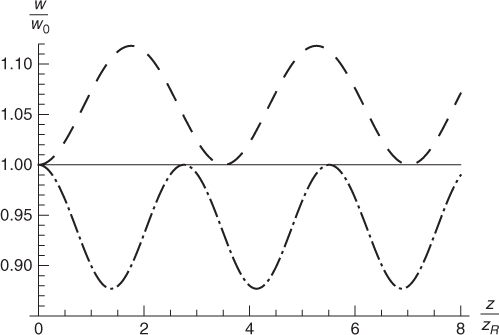
and ![]() . Equation 2.20 shows that [5] when P0 < Pc the beam diffraction initially overcomes the beam-induced index well: the beam initially expands, with w/w0 oscillating between a maximum (Pc/P0)1/2 and a minimum equal to one; when P0 > Pc, the reverse happens and the beam initially contracts, with w/w0 breathing between a maximum (unity) and a minimum (Pc/P0)1/2. These two cases correspond to optical breathers4. When P0 = Pc, diffraction is exactly balanced by nonlinearity, and the Gaussian-shaped beam preserves its width as it travels in a straight path along z. This is an optical soliton. The evolution of an individual Gaussian beam for various powers P0 is shown in Figure 2.1.
. Equation 2.20 shows that [5] when P0 < Pc the beam diffraction initially overcomes the beam-induced index well: the beam initially expands, with w/w0 oscillating between a maximum (Pc/P0)1/2 and a minimum equal to one; when P0 > Pc, the reverse happens and the beam initially contracts, with w/w0 breathing between a maximum (unity) and a minimum (Pc/P0)1/2. These two cases correspond to optical breathers4. When P0 = Pc, diffraction is exactly balanced by nonlinearity, and the Gaussian-shaped beam preserves its width as it travels in a straight path along z. This is an optical soliton. The evolution of an individual Gaussian beam for various powers P0 is shown in Figure 2.1.
Figure 2.1 Evolution of Gaussian beams in a strongly nonlocal Kerr medium. The initial beam width is the same in all cases, but the input powers are different: dashed line P0/Pc = 0.8, solid line P0/Pc = 1.0, dashed-dot line P0/Pc = 1.3.
For P0 = Pc, w = w0, c = 0, and β0 = 1/zR, where ![]() is the Rayleigh distance; Equation 2.24 simplifies to the expression of an accessible soliton [5]5
is the Rayleigh distance; Equation 2.24 simplifies to the expression of an accessible soliton [5]5
where ![]() . ϕz is the phase shift of the slowly varying envelope Ψ after propagating over a distance z. An accessible (spatial) soliton with arbitrary width can propagate as long as its power P0 exactly equals the critical value Pc defined in Equation 2.23.
. ϕz is the phase shift of the slowly varying envelope Ψ after propagating over a distance z. An accessible (spatial) soliton with arbitrary width can propagate as long as its power P0 exactly equals the critical value Pc defined in Equation 2.23.
The phase shift of an accessible soliton can be very large [30], as it stems from the phase difference ϕ given by Equation 2.18, as discussed in Section 2.2.2.2. The large phase shift of nonlocal spatial optical solitons in lead glasses, media with an infinite range of nonlocality [16], was recently confirmed experimentally [35].
The comparison between the analytical solutions and the numerical simulations of Equation 2.4 for various w0/wm and P0 shows that [30] the analytical predictions are close (the absolute values of the relative errors are within 10%) to the simulations for w0/wm of about 0.5. For the same w0/wm, the higher the input power, the better the approximation. It was also proved by both the variational approach [36] and a perturbation method [37] that the single soliton solution of the NNLSE (Eq. 2.4) with the regular response function is exactly the Gaussian soliton (Eq. 2.26) when ![]() . However, this is not the case for an irregular response function, as discussed in Section 2.3.
. However, this is not the case for an irregular response function, as discussed in Section 2.3.
2.2.4 Breather and Soliton Clusters of the Snyder–Mitchell Model
We search for solutions of the Snyder–Mitchell model (Eq. 2.17) by writing it as a product of ![]() and the Gaussian function
and the Gaussian function ![]() given by Equation 2.19
given by Equation 2.19
Substitution of Equation 2.27 into Equation 2.17 yields
The solutions ψF of Equation 2.28 have different forms in different coordinate systems and constitute breather and soliton clusters of the Snyder–Mitchell model: the Hermite–Gaussian (HG) cluster in the Cartesian coordinate system [38, 39], the Laguerre–Gaussian (LG) cluster in the cylindrical coordinate system [40–42], and the Ince–Gaussian (IG) cluster [43, 44] in the elliptic coordinate system, as well as the Hermite–Laguerre–Gaussian (HLG) cluster [45].
Soliton clusters have been obtained not only exactly analytically in the framework of the Snyder–Mitchell model (Eq. 2.17) [strong nonlocality with a regular response function ![]() ], as mentioned in the paragraph earlier, but also approximately analytically and numerically in the other cases with arbitrary degrees of nonlocality modeled by the NNLSE (Eq. 2.4), regardless of a regular or irregular response function
], as mentioned in the paragraph earlier, but also approximately analytically and numerically in the other cases with arbitrary degrees of nonlocality modeled by the NNLSE (Eq. 2.4), regardless of a regular or irregular response function ![]() . Among them, we mention LG0m-type ring vortex solitons [46], LGnm-type solitons [27], HGnm-type and LGnm-type solitons as well as the transformations between them [47], and rotating HLG-type solitons [48, 49]. All of them are soliton clusters in nonlocal nonlinear media with a phenomenological regular Gaussian response function. In physically real media with an irregular response function, there also exist the (1 + 1)-D HG-type multipole soliton cluster [50–52], the (1 + 2)-D vortex soliton cluster6 [16, 53], and HGnm-type soliton cluster [54]. The stability of these structures critically depends on the spatial profile of the response function
. Among them, we mention LG0m-type ring vortex solitons [46], LGnm-type solitons [27], HGnm-type and LGnm-type solitons as well as the transformations between them [47], and rotating HLG-type solitons [48, 49]. All of them are soliton clusters in nonlocal nonlinear media with a phenomenological regular Gaussian response function. In physically real media with an irregular response function, there also exist the (1 + 1)-D HG-type multipole soliton cluster [50–52], the (1 + 2)-D vortex soliton cluster6 [16, 53], and HGnm-type soliton cluster [54]. The stability of these structures critically depends on the spatial profile of the response function ![]() [12, 55].
[12, 55].
2.2.5 Complex-Variable-Function Gaussian Breathers and Solitons
A complex-variable-function (CVF) Gaussian beam is the solution of Equation 2.17 in the form ![]() , where ψG is the Gaussian function given by Equation 2.19 and ψC satisfies Equation 2.28. To obtain this solution, we first introduce a rotating coordinate system (x′, y′, z) in the transverse plane perpendicular to the z axis: x′ = w0[xcos(ϑ(z)) + ysin(ϑ(z))]/w(z) and y′ = w0[ycos(ϑ(z)) − xsin(ϑ(z))]/w(z), where dϑ(z)/dz denotes the angular velocity (the angular rotation per unit propagation distance) and w(z) is given by Equation 2.20. In the rotating coordinate system, Equation 2.28 can be written as [56, 57]
, where ψG is the Gaussian function given by Equation 2.19 and ψC satisfies Equation 2.28. To obtain this solution, we first introduce a rotating coordinate system (x′, y′, z) in the transverse plane perpendicular to the z axis: x′ = w0[xcos(ϑ(z)) + ysin(ϑ(z))]/w(z) and y′ = w0[ycos(ϑ(z)) − xsin(ϑ(z))]/w(z), where dϑ(z)/dz denotes the angular velocity (the angular rotation per unit propagation distance) and w(z) is given by Equation 2.20. In the rotating coordinate system, Equation 2.28 can be written as [56, 57]
where ![]() and
and ![]() . The solution of Equation 2.29 is found to be [57]
. The solution of Equation 2.29 is found to be [57]
where ![]() denotes an arbitrary analytical function [ζ±′ = (x′ ± iy′)/(b w0)], b ≠ 0 is an arbitrary real parameter, θ(2)(z) is given by Equation 2.22, and ‘‘ + ( − )" represents the rotation direction consistent with the right-hand (left-hand) rule relative to the direction of propagation.
denotes an arbitrary analytical function [ζ±′ = (x′ ± iy′)/(b w0)], b ≠ 0 is an arbitrary real parameter, θ(2)(z) is given by Equation 2.22, and ‘‘ + ( − )" represents the rotation direction consistent with the right-hand (left-hand) rule relative to the direction of propagation.
From the solution (Eq. 2.30) of Equation 2.29, one can obtain the solution of Equation 2.17 in the laboratory frame [57]:
where C0 is a constant to be determined from ![]() and
and ![]() . The solution is referred to as a CVF Gaussian beam owing to the fact that f(ζ+) is an arbitrary analytical CVF. The structure of the beam is determined by the product of the function f(ζ) and a Gaussian function. If observed in the laboratory frame (x, y, z), the trajectories of the corresponding points of the beam generally rotate during propagation.
. The solution is referred to as a CVF Gaussian beam owing to the fact that f(ζ+) is an arbitrary analytical CVF. The structure of the beam is determined by the product of the function f(ζ) and a Gaussian function. If observed in the laboratory frame (x, y, z), the trajectories of the corresponding points of the beam generally rotate during propagation.
The parameter b, a distribution factor, describes the transverse distribution of the CVF Gaussian beam. The distribution is farther from the beam center for smaller b and is clustered more closely around the beam center for larger b [57].
The CVF Gaussian beam can form either breathers or solitons for different input powers P0; it evolves similarly to the Gaussian beam [5, 30]. When P0 = Pc, Equation 2.31 can reduce to [56]
2.32 ![]()
where ζ±(s) = (x ± iy)exp( ± iz/zR)/(bw0). This is a CVF Gaussian soliton, where diffraction is exactly balanced by nonlinearity. Its transverse distribution is preserved but rotates as the CVF Gaussian soliton travels along the propagation axis.
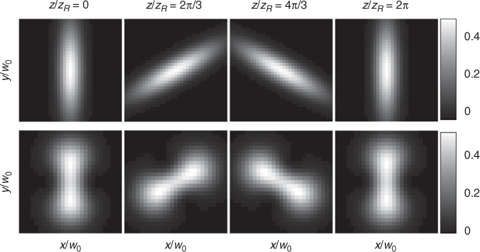
Figure 2.2 shows the evolution of the Gaussian CVF Gaussian soliton [f(x) = exp( − x2/2)] and the fourth-order Hermite CVF Gaussian soliton [f(x) = H4(x), where Hn(x) is the nth-order Hermite polynomial]. It can be found that the pattern of the Gaussian CVF Gaussian soliton consists of a rotating elliptic Gaussian soliton and that of the fourth-order Hermite CVF Gaussian soliton is something similar to a rotating figure 8 when b = 1.5.
Figure 2.2 Dynamics of the Gaussian CVF Gaussian soliton (the upper panels) and the fourth-order Hermite CVF Gaussian soliton (the lower panels) for b = 1.5.
There also exists another kind of stable rotating mode in nonlocal nonlinear media, the azimuthons [58]. These are not discussed in detail here. An example of azimuthons is briefly discussed in Chapter 6.
2.2.6 Self-Induced Fractional Fourier Transform
The fractional Fourier transform (FRFT), which can show the characteristics of the signal continuously changing from the spatial domain to the spectral domain, was introduced in optics in 1993 [59]. Traditionally, the FRFT is optically performed by linear devices such as lenses and quadratic graded-index media. Here, we show that the FRFT naturally exists in strongly nonlocal nonlinear media described by the Snyder–Mitchell model; the propagation of optical beams in these media can be simply regarded as a self-induced FRFT [60].
For the (1 + 2)-D case, in cartesian coordinates the eigen-solution of Equation 2.17 is the HG soliton cluster [38, 39], that is, ![]() , and
, and
In Equation 2.33, q( = 0, 1, 2, … ) is the order of the solution corresponding to the soliton eigenvalue [60]:
Mathematically, ![]() is the eigen function of the FRFT (represented as
is the eigen function of the FRFT (represented as ![]() ) [59, 61]:
) [59, 61]: ![]() where the order of the FRFT is γ = z/zR. It is well known that an arbitrary square-integrable input field can be expressed as a linear superposition of the eigen-soliton solutions, that is,
where the order of the FRFT is γ = z/zR. It is well known that an arbitrary square-integrable input field can be expressed as a linear superposition of the eigen-soliton solutions, that is, ![]() . According to the linearity of Equation 2.17 and the FRFT, the propagation of an arbitrary beam in strongly nonlocal nonlinear media described by the Snyder–Mitchell model can be regarded as the self-induced FRFT of the input field
. According to the linearity of Equation 2.17 and the FRFT, the propagation of an arbitrary beam in strongly nonlocal nonlinear media described by the Snyder–Mitchell model can be regarded as the self-induced FRFT of the input field
2.35 ![]()
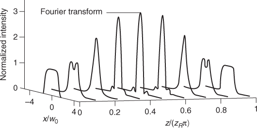
The physical origin of this effect is as follows: when a beam is launched in the medium, it would induce a quadratic graded-index channel owing to strong nonlocality. The propagation in the channel then performs the FRFT [59], as shown in Figure 2.3. As the gradient of the refractive index distribution can be controlled by the power, the order of the self-induced FRFT can be controlled by the input power in addition to the propagation distance z, quite differently from the traditional linear FRFT devices.
Figure 2.3 Propagation dynamics of the super–Gaussian field ![]() in strongly nonlocal nonlinear media with a Gaussian response function.
in strongly nonlocal nonlinear media with a Gaussian response function.
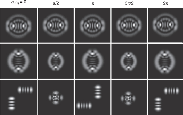
According to the properties of the FRFT, the behavior of beams in strongly nonlocal nonlinear media can be conveniently predicted. Here, we discuss three special cases:
Figure 2.4 Dynamics of building-block-like solitons (the first row), building-block-like breathers (the second row), and multi-soliton interactions (the third row) in strongly nonlocal nonlinear media with Gaussian response function based on numerical simulation of the NNLSE (Eq. 2.4).
2.3 Nonlocal Spatial Solitons in Nematic Liquid Crystals
NLC is the first optical nonlinear material with a large enough characteristic length to mimic the strongly nonlocal regime [14, 15]. Spatial solitons in NLC, so-called nematicons [6], are the first accessible soliton observed in experiments [15]. The nonlocal nonlinearity in NLC comes from optically induced molecular reorientation. Although some features of nematicons can be explained by the Snyder–Mitchell model [5], others are unique, for instance the voltage-controllable degree of nonlocality [62] and mutual interactions [63].
In this section we discuss the properties of optical beams propagating in NLC-filled planar cells with an external bias voltage but without considering the boundary effects; we address the model and the approximate analytic solution for a single nematicon, as well as nonlocality-controlled interactions [63], short-range interactions [29], and long-range interactions [64] between two nematicons. The boundary effects of the cell on nematicon propagation are addressed in Chapters 11 and 15.
2.3.1 Voltage-Controllable Characteristic Length of NLC
The physical mechanism of the nonlinearity in NLC is optically induced molecular reorientation; the nonlocality comes from interactions between NLC molecules. The dynamics of reorientation in NLC-filled cells is somewhat complicated; with some approximations, however, the NLC nonlinear response function can be found [63, 65].
Let us consider the planar geometry of NLC-filled cells as described in previous works [14, 66]. NLC, anchored at the boundaries along the x coordinate (thickness), is a positive uniaxial with extraordinary index n|| and ordinary index ![]() (
(![]() ). In the presence of an externally applied (low-frequency) electric field Erf, the propagation of the slowly varying envelope Ψ of a light beam linearly polarized along x (an extraordinary wave) and propagating along z can be described by the system [14, 66]
). In the presence of an externally applied (low-frequency) electric field Erf, the propagation of the slowly varying envelope Ψ of a light beam linearly polarized along x (an extraordinary wave) and propagating along z can be described by the system [14, 66]
where θ is the tilt angle of the NLC molecules and θ0 is the peak-tilt in the absence of light, K is the NLC average elastic constant, k = k0n0 with k0 the vacuum wavenumber and ![]() is the refractive index of the extraordinary light,
is the refractive index of the extraordinary light, ![]() and
and ![]() ) are optical and low frequency dielectric anisotropies, respectively. The term
) are optical and low frequency dielectric anisotropies, respectively. The term ![]() in Equation 2.37 was proven to be negligible compared to
in Equation 2.37 was proven to be negligible compared to ![]() [65, 66]; therefore it can be removed. The planar boundaries and anchoring at the interfaces define θ|x=−L/2 = θ|x=L/2 = 0, where L is the cell thickness. In the absence of light, the pretilt angle
[65, 66]; therefore it can be removed. The planar boundaries and anchoring at the interfaces define θ|x=−L/2 = θ|x=L/2 = 0, where L is the cell thickness. In the absence of light, the pretilt angle ![]() is symmetric along x about x = 0 (the cell center) and depends only on x [66]
is symmetric along x about x = 0 (the cell center) and depends only on x [66]
Furthermore, we can set ![]() , with Φ being the optically induced perturbation. Noting that
, with Φ being the optically induced perturbation. Noting that ![]() and
and ![]() in the middle of the cell when the beam width is far smaller than the cell thickness, we can simplify Equations 2.36 and 2.37 into the following system, which describes the coupling between Ψ and Φ [62, 66]
in the middle of the cell when the beam width is far smaller than the cell thickness, we can simplify Equations 2.36 and 2.37 into the following system, which describes the coupling between Ψ and Φ [62, 66]
where the parameter wm (wm > 0 for |θ0| ≤ π/2), that is, the characteristic length of the nonlinear response function [63], reads
For a symmetric geometry and ignoring the boundary effects, Equation 2.40 has a particular solution in the form of a convolution integral of |Ψ|2 with the function R
2.42 ![]()
with R in the (1 + 2)-D case given by Hu et al. [63]
where K0 is the zeroth order modified Bessel function of the second kind; R in the (1 + 1)-D case is [65]
Equations 2.39 and 2.40 can be integrated into the NNLSE (Eq. 2.4) with the nonlinear-index coefficient n2 given by Peccianti et al. [62, 64]7
and the nonlinear response function R expressed by Equation 2.43 or 2.44.
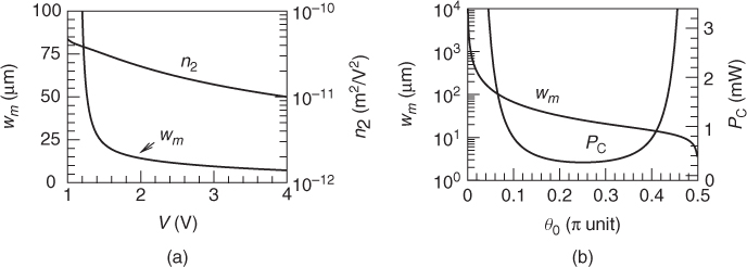
A monotonous function of θ0 on Erf is described by Equation 2.38, and it can be approximated as θ0 ≈ (π/2)[1 − (EFR/Erf)3] when Erf is larger than the Fréedericksz threshold EFR [62]. Therefore, we can clearly see from Equations 2.41 and 2.45 that wm and n2 are determined by Erf (or the bias V), or equivalently by the peak-pretilt θ0 for a given NLC cell configuration, as shown in Figure 2.5. Increasing the bias above threshold, θ0 grows monotonously from 0 to π/2, wm decreases monotonously from infinite to 0, and n2 decreases monotonously, as well. This corresponds to a voltage-controlled change of the NLC characteristic length. As a result, a voltage-controlled degree of nonlocality through the pretilt θ0 can be conveniently achieved for a fixed w0. It is important that the characteristic length of the NLC nonlinear optical response can be varied by changing the pretilt angle via a bias voltage [62]. The typical wm for an 80-μm-thick NLC cell is wm = 25.3 μm for θ0 = π/4 [63], with a nematicon width about ![]() m in experiments.
m in experiments.
Figure 2.5 (a) NLC characteristic length wm and nonlinear-index coefficient n2 versus bias voltage V. (b) Characteristic length wm and critical power of a single soliton versus pretilt angle θ0. The parameters are for an 80-μm-thick cell filled with TEB30A, as in Reference [63].
In summary, if the beam width is far smaller than the thickness of the NLC-filled cell with a bias-induced pretilt, the middle region of the cell can be considered as an infinite NLC medium with a uniform but electrically adjustable pretilt θ0; the behavior of a paraxial light beam in this region can be described by the NNLSE (Eq. 2.4) with a nonlinear coefficient n2 given by Equation 2.45 and a nonlinear response function R represented by Equation 2.43 or 2.44.
2.3.2 Nematicons as Strongly Nonlocal Spatial Solitons
As discussed in Section 2.3.1, the propagation of nematicons can be described by the NNLSE (Eq. 2.4) and the characteristic length of the NLC nonlinear optical response can be of the order of 10 μm. Therefore, a strong nonlocality can be achieved for beams of micron-scale width. The crucial difference, however, between the phenomenological response function and the NLC response function is that the NLC response function ![]() for both the (1 + 2)-D (Eq. 2.43) and the (1 + 1)-D cases (Eq. 2.44) has a singularity at the origin
for both the (1 + 2)-D (Eq. 2.43) and the (1 + 1)-D cases (Eq. 2.44) has a singularity at the origin ![]() . As a matter of fact, the phenomenological regular response function, for example, Gaussian, is nonphysical although extremely instructive, whereas the response functions of physically real materials are irregular. A regular response function for a real material has not been found so far, to say the least. Here, we rigorously show that the nonlinear induced refractive index
. As a matter of fact, the phenomenological regular response function, for example, Gaussian, is nonphysical although extremely instructive, whereas the response functions of physically real materials are irregular. A regular response function for a real material has not been found so far, to say the least. Here, we rigorously show that the nonlinear induced refractive index ![]() n determined by Equation 2.2 cannot be simplified as a quadratic self-induced index well if the response function R is irregular, no matter how strong the nonlocality is; in other words, the NNLSE (Eq. 2.4) with an irregular response function cannot be generally reduced to the Snyder–Mitchell model (Eq. 2.17 or 2.16).
n determined by Equation 2.2 cannot be simplified as a quadratic self-induced index well if the response function R is irregular, no matter how strong the nonlocality is; in other words, the NNLSE (Eq. 2.4) with an irregular response function cannot be generally reduced to the Snyder–Mitchell model (Eq. 2.17 or 2.16).
Let us take the (1 + 1)-D case as an example. For a symmetric response function and a strong nonlocality, one can expand Equation 2.2 about x = 0 and obtain
where ![]() n(0) = ∫|Ψ(ξ, z)|2R(ξ)dξ ≈ R0P0,
n(0) = ∫|Ψ(ξ, z)|2R(ξ)dξ ≈ R0P0, ![]() n′(0) = − ∫|Ψ(ξ, z)|2R′(ξ)dξ = 0 [Ψ(ξ, z) is symmetric or antisymmetric about ξ], and
n′(0) = − ∫|Ψ(ξ, z)|2R′(ξ)dξ = 0 [Ψ(ξ, z) is symmetric or antisymmetric about ξ], and ![]() n′′(0) = ∫|Ψ(ξ, z)|2R′′(ξ)dξ. If R(x) is regular, it can be found that
n′′(0) = ∫|Ψ(ξ, z)|2R′′(ξ)dξ. If R(x) is regular, it can be found that ![]() n′′(0) ≈ R′′(0)P0, then we get a quadratic self-induced index well. If R(x) has a singularity in x = 0, for example, in NLC, R′′(x) satisfies
n′′(0) ≈ R′′(0)P0, then we get a quadratic self-induced index well. If R(x) has a singularity in x = 0, for example, in NLC, R′′(x) satisfies ![]() , then we can have
, then we can have ![]() . It can also be found that
. It can also be found that ![]() (strong nonlocality),8 then
(strong nonlocality),8 then
![]()
Therefore, only for symmetric soliton solutions (|Ψ(0, z)|2 is nonzero and not a function of z), we can have a quadratic self-induced index well. Apart from this, either ![]() n(x, z) will be a function of z for breather solutions or a higher order nonzero term should be taken into account in the expansion (Eq. 2.46) for antisymmetric solutions, because |Ψ(0, z)|2 = 0. The discussion earlier above for the (1 + 1)-D case is instructive, although the (1 + 2)-D case is somewhat more complicated.
n(x, z) will be a function of z for breather solutions or a higher order nonzero term should be taken into account in the expansion (Eq. 2.46) for antisymmetric solutions, because |Ψ(0, z)|2 = 0. The discussion earlier above for the (1 + 1)-D case is instructive, although the (1 + 2)-D case is somewhat more complicated.
In order to investigate this issue further, we take the higher order term of the expansion into consideration and obtain, for both the (1 + 1)-D and the (1 + 2)-D cases [37, 67–69],
where ![]() and χn = V(n)(r)/n! It was shown that, if the response function is regular, and if χ4 and χ6 in Equation 2.47 approach zero when wm/w0 → ∞, Equation 2.4 rigorously converges to Equation 2.17 [37, 67]. However, for the response function with a singularity, that is, Equation 2.43 or 2.44 in NLC, χ4 and χ6 are free from the characteristic length wm [37, 69]. Even when the characteristic length wm approaches infinity, χ4 and χ6 still remain finite and do not tend to zero. It can be found that the ratio of the third term to the second term in Equation 2.47, χ4r2/χ2, is about
and χn = V(n)(r)/n! It was shown that, if the response function is regular, and if χ4 and χ6 in Equation 2.47 approach zero when wm/w0 → ∞, Equation 2.4 rigorously converges to Equation 2.17 [37, 67]. However, for the response function with a singularity, that is, Equation 2.43 or 2.44 in NLC, χ4 and χ6 are free from the characteristic length wm [37, 69]. Even when the characteristic length wm approaches infinity, χ4 and χ6 still remain finite and do not tend to zero. It can be found that the ratio of the third term to the second term in Equation 2.47, χ4r2/χ2, is about ![]() for (1 + 1)-D geometries [
for (1 + 1)-D geometries [![]() and
and ![]() , as given in Reference 37] and
, as given in Reference 37] and ![]() for (1 + 2)-D geometries [
for (1 + 2)-D geometries [![]() and
and ![]() , as in Reference 69] in the strong nonlocal case, which means that the third term in Equation 2.47 cannot be ignored when r ∼ w0. Therefore, the influence of χ4 should be accounted for and the profile of the fundamental nematicon does not approach a Gaussian function even if the nonlocality is strong.
, as in Reference 69] in the strong nonlocal case, which means that the third term in Equation 2.47 cannot be ignored when r ∼ w0. Therefore, the influence of χ4 should be accounted for and the profile of the fundamental nematicon does not approach a Gaussian function even if the nonlocality is strong.
A perturbation method can be used to find an approximate analytical solution irrespective of whether the response function is regular or not [37, 67]. To the first-order perturbation, the (1 + 2)-D perturbed solution of a single soliton of Equation 2.4 in NLC is (details can be found in Appendix 2.B)
where σ ≈ 1.44, a ≈ 0.076, and b ≈ 0.022. The profile of the solution (Eq. 2.48) is not Gaussian except for both a = 0 and b = 0, and its FWHM [full width at half (intensity) maximum] is wFWHM ≈ 1.841w0, whereas the FWHM of the Gaussian function is ![]() . The relative error between the corresponding powers carried by the soliton of Equation 2.48 and by the Gaussian soliton (a = b = 0 in Eq. 2.48) with the same FWHM is as high as 50%, and the profile given by Equation 2.48 is more accurate than Gaussian, as discussed in the Appendix 2.B.
. The relative error between the corresponding powers carried by the soliton of Equation 2.48 and by the Gaussian soliton (a = b = 0 in Eq. 2.48) with the same FWHM is as high as 50%, and the profile given by Equation 2.48 is more accurate than Gaussian, as discussed in the Appendix 2.B.
2.3.3 Nematicon–Nematicon Interactions
Nematicon–nematicon interactions are drastically influenced by the nonlocality of the nonlinear response. For a local Kerr-type nonlinearity, two coherent bright solitons attract (or repel) each other when they are in phase (or out of phase), and the interaction only occurs when the two solitons overlap [1]. In the strongly nonlocal case, it was shown theoretically and experimentally that attraction can take place between bright solitons with any phase difference [5, 63, 65, 70]. Additionally, two solitons can be mutually trapped via the strong nonlocality when their fields do not overlap, which is called long-range interaction. Short-range interactions can describe interacting solitons with nonzero overlap.
Similar to strongly nonlocal solitons, interacting nematicons can exhibit some peculiar features, such as a voltage-controllable attraction/repulsion [63]. In this section, we summarize a few experimental results on nematicon–nematicon interactions, including nonlocality-controlled interactions [63] and short- [29] and long-range interactions [64].
2.3.3.1 Voltage-Controllable Interaction
The interaction of two spatial solitons depends on the phase difference between them, their coherence and the nonlinear nonlocality [1, 5]. In the local case, two in-phase solitons attract each other and two out-of-phase solitons repel. On the other hand, if the nonlocality of the nonlinear material is strong enough, the soliton interaction is always attractive, independent of their phase difference [5, 70, 71]. Thus, two out-of-phase solitons can repel or attract one another, depending on whether the nonlocality degree is below or above a threshold. The interaction dependence on nonlocality was theoretically described by Rasmussen et al. [65].
As shown in Equation 2.41 and Figure 2.5, the characteristic length of the NLC nonlinear response can vary by acting on the pretilt angle via a bias voltage. For a given beam width, the degree of nonlocality can be changed continuously by wm through the bias. As a result, a voltage-controlled nonlocality can be conveniently achieved through the NLC pretilt θ0. Then, a voltage-controlled interaction between nematicons can be performed, with potential applications in all-optical signal processing devices.
The voltage-controllable interaction was first observed experimentally in Reference 63. After Hu et al. [63], Figure 2.6 shows the influence of the pretilt θ0 (or equivalently the degree of nonlocality for a fixed w0) on the interaction between two nematicons. One can see that for θ0 ≤ π/4 the nonlocality is strong enough to ensure attraction of both in-phase and out-of-phase solitons. However, when θ0 = 0.45π and the degree of nonlocality reduces, out-of-phase solitons begin to repel each other whereas in-phase solitons keep attracting.
Figure 2.6 Numerical simulations of the interaction between in-phase and out-of-phase solitons based on Equations 2.36 and 2.37. The width of each soliton is 4 μm and the input power is 1.1mW. The separation and the relative angle between the two solitons are 12 μm and 0.57°(tan0.57° = 0.01), respectively. Source: Reprinted with permission from W. Hu, et al. Appl. Phys. Lett., 89:071111, 2006. Copyright 2006, American Institute of Physics.

The experimental results are shown in Figure 2.7. When the bias V = 1.4 V (θ0 ≈ π/4), the photos of in-phase and out-of-phase solitons are almost the same. It means for θ0 = π/4, the degree of nonlocality is strong enough to eliminate the interaction dependence on the phase difference between solitons. In this case, wm ≈ 25.3 μm, which is larger than the separation of the two beams.
Figure 2.7 Photos of soliton pair propagating in the NLC cell. The applied biases are 1.0 V, 1.4 V, and 2.4 V, corresponding to pretilt angles of 0.01π, 0.25π, and 0.45π, respectively. Source: Reprinted with permission from Hu et al. Appl. Phys. Lett., 89:071111, 2006. Copyright 2006, American Institute of Physics.
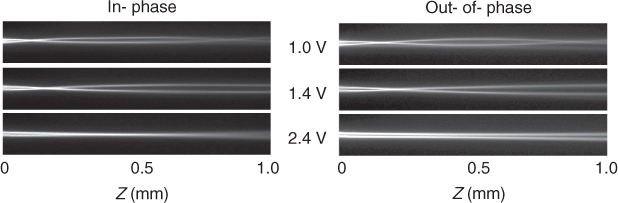
For a bias V = 1.0 V slightly lower than the Fréedericksz threshold, Vt = 1.14 V (a small tilt eases reorientation even at voltages below the threshold [62]), the pretilt θ0 is nearly zero, and the nonlocality is much stronger than when V = 1.4 V. For this reason, a second crossing point is observed for both in-phase and out-of-phase solitons.
When the bias V(pretilt angle θ0) is increased, the degree of nonlocality wm/w0 and the characteristic length wm decrease. For V = 2.4 V (θ0 ≈ 0.45π), we have wm ≈ 11 μm, which approximately equals the separation between the two solitons. In this case, we observe attraction of in-phase solitons and repulsion of out-of-phase solitons. We also see the two in-phase solitons merge into one soliton, qualitatively similar to that observed in the numerical simulations in Figure 2.6.
2.3.3.2 Short-Range Interaction
For the strongly nonlocal case, two solitons always attract each other regardless of the phase difference between them, at variance with the local solitons. However, the phase difference can still influence the interaction when two solitons have a nonzero overlap, that is, for short-range interactions. From conservation of linear momentum, the trajectory of two nematicons can be controlled by the phase difference between them. This steering phenomenon controlled by the phase difference could be used in all-optical information processing.
Phase-dependent short-range interactions were first predicted and experimentally confirmed by Hu et al. [29]. For short-range interactions, the two solitons can attract each other and propagate together. Equation 2.10 implies that the trajectory of the center of mass is a straight line with slope determined by ![]() with respect to the z axis. For the NNLSE (Eq. 2.4), let us take two simultaneously incident Gaussian solitons of width w0 that are coplanar in the x–z plane, with a phase difference γ and a separation d( = 2h), that is,
with respect to the z axis. For the NNLSE (Eq. 2.4), let us take two simultaneously incident Gaussian solitons of width w0 that are coplanar in the x–z plane, with a phase difference γ and a separation d( = 2h), that is,
where α is the incident angle with respect to the z axis and the amplitude Ψ0 is sufficiently large for the two beams to propagate as solitons. For the initial condition (Eq. 2.49), the total beam power is
2.50 ![]()
the momentum
2.51 ![]()
and the initial position of the center of mass rc0 = 0. Let βx be the angle of the trajectory of the center of mass with respect to the z axis; then the slope tanβx = Mx/P is
and tanβy = 0, where Θ = 1/kw0 is the far-field divergence of a Gaussian beam.
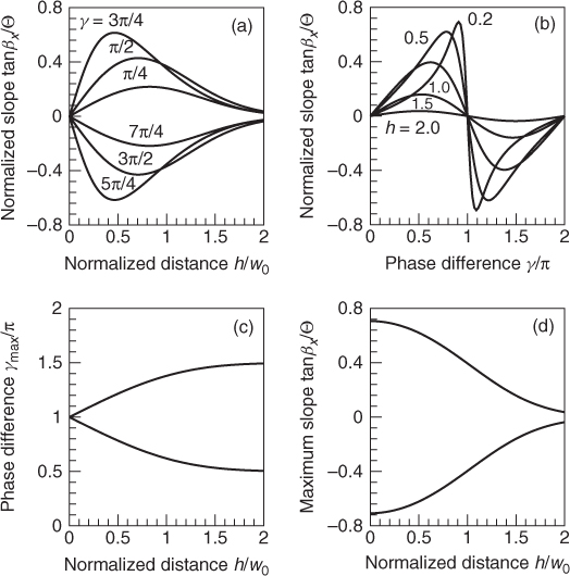
As visible in Figure 2.8a and b, the slope of trajectory of the center of mass is highly dependent on the separation 2h and the phase difference γ. It shows that tanβx = 0 only when γ = 0 or π for ![]() , and tanβx goes to zero when
, and tanβx goes to zero when ![]() . tanβx has a significant value when h is comparable or smaller than the beam width w0. It can be seen in Figure 2.8c and 2.8d that the maximum tilting angle occurs when γ approximates π for a small distance h. Therefore, the steering angle of the whole beam is significant only for thin beams. It is important to emphasize that the analytical result for the motion of the center of mass (Eq. 2.52) is universal and independent of the form of the nonlinear response function R. This means that, no matter what the material, the degree of nonlocality, and the input power of the beams are, the motion of the center of mass is the same as that in the initial condition (Eq. 2.49).
. tanβx has a significant value when h is comparable or smaller than the beam width w0. It can be seen in Figure 2.8c and 2.8d that the maximum tilting angle occurs when γ approximates π for a small distance h. Therefore, the steering angle of the whole beam is significant only for thin beams. It is important to emphasize that the analytical result for the motion of the center of mass (Eq. 2.52) is universal and independent of the form of the nonlinear response function R. This means that, no matter what the material, the degree of nonlocality, and the input power of the beams are, the motion of the center of mass is the same as that in the initial condition (Eq. 2.49).
Figure 2.8 Dependence of the slope on distance h (a) and phase difference γ (b) for two parallel-injected solitons. (c) Phase difference γmax for the maximum slope angle versus distance h and (d) maximum tilt angle tan(βx) versus distance h. α = 0 for all of the figures.
The experimental results are shown in Figure 2.9; see Reference 29. In Figure 2.9a and b, each of the two solitons is launched alone in the NLC cell and their trajectories are found to be straight and horizontal. When two solitons are injected simultaneously, they propagate as a whole, and tilt (c) up or (d) down in the x direction. As the separation is so small that the two solitons cannot be distinguished with the microscope, one can see a bound-beam state steered by the phase difference γ.
Figure 2.9 Photos of beam trajectories for single solitons [(a) and (b)] and two solitons injected together [(c) and (d)] propagating in the NLC cell. The phase differences between the two solitons for (c) and (d) are about π/2 and 3π/2, respectively. (e) Tilting angle of two beams versus phase difference between them. Square points: experiment results; solid curve: theoretical fitting from Equation 2.52.
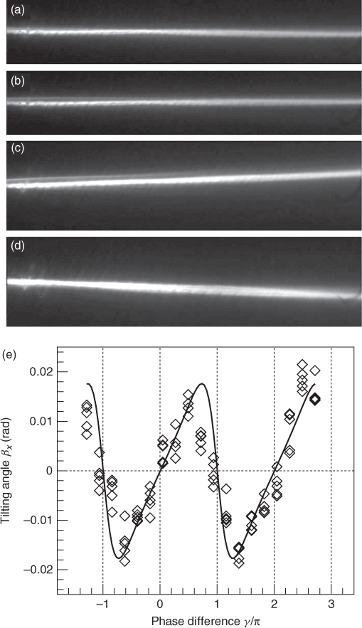
The quantitative comparison between the experimental measurements and the theoretical predictions are shown in Figure 2.9e. One can see that the experimental points are located around the theoretical prediction with a relatively small random error. The latter is mainly due to slight variations in phase difference γ. Except for these random errors, the experimental results agree well with the theoretical prediction.
2.3.3.3 Long-Range Interaction
The long-range interaction is a feature of strongly nonlocal solitons, which was first observed in NLC [70] and in lead glass [72]. In strongly nonlocal media, two solitons separated far away can attract via the nonlocal nonlinear response, no matter what their phase difference is. The range of interaction is limited by the range of the nonlocal nonlinearity. The interaction between nematicons separated by 43 times the beam width (the full width at half-maximum) was demonstrated experimentally and reported by Cao et al. [64].
The distance Γ from the input plane to the first collision point of two solitons is used to indicate the strength of the interaction between them. The shorter Γ is, the stronger is the interaction. Figure 2.10a shows experimental results for an initial separation d0 = 27.3 μm, that is, about 10 times the initial beam width w0 (w0 = 3.0 μm). The launch power of a single beam is maintained at 9.4 mW. The trajectories of two solitons are acquired by a CCD camera as the bias voltage is increased from 0.8 to 1.9 V. When the voltage is about 1.2 V, that is, close to Vπ/4 ≈ 1.4 V to make the pretilt θ0 = π/4, Γ reaches its minimum. It indicates that the interaction between nematicons is the strongest when the pretilt is nearly π/4.
Figure 2.10 Photos of beam traces for solitons colliding in NLC: the crossing points vary with the bias voltage V (a) or the incident power P0 (b). The initial separation between beams is 27.3 μm in (a) and 115 μm in (b).
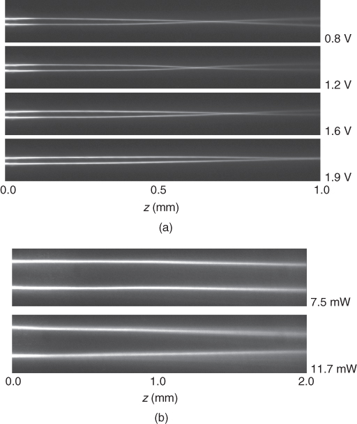
Then the separation between nematicons is increased to implement long-range interactions at the optimum bias, which is set to 1.2 V. As shown in Figure 2.10b, when d0 is up to 115 μm, that is, d0 ≈ 72w0 (w0 = 1.6 μm, and the full width at half-maximum is about 2.67 μm), at low input power (P0 = 7.5 mW) the attraction is almost absent. When the input power is high enough, that is, P0 = 11.7 mW, attraction is observed. Please note that d0 = 115 μm is larger than both the thickness of the NLC cell (80 μm) and the characteristic length wm = 25.3 μm when θ0 = π/4 [63]. As the characteristic length wm is limited by the thickness of the cell, the long-range interaction between nematicons is also limited by it.
2.4 Conclusion
In this chapter, we discussed the propagation of spatial optical solitons in nonlocal nonlinear media. The dynamics of paraxial optical beams is modeled in nonlocal Kerr media by the NNLSE (Eq. 2.4).
The Snyder–Mitchell model is the simplified version of the NNLSE for the limit of the strong nonlocality and with the response function symmetric and regular at its origin. The Snyder–Mitchell model can support HG breathers and solitons, one specific case of which is the accessible soliton suggested by Snyder and Mitchell, LG breathers and solitons, and IG breathers and solitons in various coordinate systems, as well as various stable rotating modes. The propagation of the optical beams in strongly nonlocal nonlinear media described by the Snyder–Mitchell model can also be simply regarded as the self-induced FRFT.
NLC is the first-found optical nonlinear material with a larger enough characteristic length to mimic the strong nonlocality. The spatial optical solitons in NLC, the so-called nematicons, are the first accessible solitons observed in experiments. If the beam width is far smaller than the thickness of the NLC-filled cell with a bias-induced pretilt, the middle region of the cell can be considered as if it were an infinite NLC medium with a uniform but electrically adjustable pretilt; the behavior of the paraxial optical beams in this region can be described by the NNLSE with a nonlinear coefficient n2 given by Equation 2.45 and a nonlinear response function being a zeroth order modified Bessel function of the second kind (Eq. 2.43) for (1 + 2)-D case or exponential-decay function (Eq. 2.44) for (1 + 1)-D case, both of which are irregular at their origins. The NNLSE with an irregular response function can generally not be reduced to the Snyder–Mitchell model. The nematicons can exhibit various interactions, including the nonlocality-controlled interactions, the short-range interactions, and the long-range interaction, all of which were experimentally confirmed.
Appendix 2.A: Proof of the Equivalence of the Snyder–Mitchell Model (Eq. 2.16) and the Strongly Nonlocal Model (Eq. 2.11)
From Equations 2.13 and 2.14, one can have the following operations:
2.A.1 ![]()
2.A.2 ![]()
where ![]() and
and ![]() are the nabla operators in the
are the nabla operators in the ![]() -coordinate and the
-coordinate and the ![]() -coordinate, respectively. Noting that
-coordinate, respectively. Noting that
![]()
and
![]()
one can get
2.A.3 ![]()
and
Substitution of Equations 2.A.4 and 2.A.4 into Equation 2.12 provides Equation 2.16.
Appendix 2.B: Perturbative Solution for a Single Soliton of the NNLSE (Eq. 2.4) in NLC
First, we give the dimensionless (normalization) transform of Equations 2.39 and 2.40. Introducing the dimensionless functions u and q, as well as the dimensionless variables X, Y, and Z,
2.B.1 ![]()
where
![]()
we get the dimensionless system
2.B.2 ![]()
2.B.3 ![]()
where ![]() , and αd = w0/wm. The substitution of the solution of Equation 2.B.3 into Equation 2.B.2 yields the dimensionless NNLSE:
, and αd = w0/wm. The substitution of the solution of Equation 2.B.3 into Equation 2.B.2 yields the dimensionless NNLSE:
where ![]() and
and ![]() is the response function in the dimensionless system. Note that we can also obtain Equation 2.B.4 directly from Equation 2.4 with Equation 2.43 via the transform (Eq. 2.B.1) and
is the response function in the dimensionless system. Note that we can also obtain Equation 2.B.4 directly from Equation 2.4 with Equation 2.43 via the transform (Eq. 2.B.1) and ![]() .
.
In order to find an approximate solution for a single soliton of Equation 2.B.4, we use the perturbation method widely employed in quantum mechanics [37, 67, 68]; see also bibliography in Reference 37, for example, which can check whether the response function is regular. The perturbed solution of Equation 2.B.4 is (see Eq. 36 in Reference 68)
2.B.5 ![]()
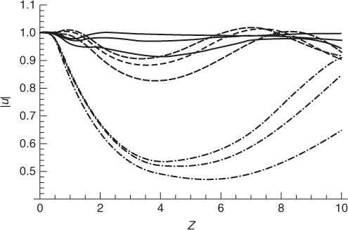
where the perturbed parameters σ ≈ 1.44, a ≈ 0.076, b ≈ 0.022, c ≈ 0.00022, and d ≈ 0.00037, and all of them are free from the degree of nonlocality αd. Figures 2.B.1 and 2.B.2 compare the numerical simulations of Equation B.4 for the various inputs u(X, Y, 0) given by Equation 2.B.5 with different order perturbation and αd. It can be observed that the Gaussian function (zero-order perturbation) has a much larger error, and the relative error (|u(0, 0, 0)| − |u(0, 0, z)|min)/|u(0, 0, 0)| is about 46% even if αd = 0.01. The first-order perturbation, however, is accurate enough with a relative error of about 12% when αd = 0.1.
Figure 2.B.1 Comparison of propagation for various inputs with different order perturbation, αd = 0.1 and μ = 1. (a) Zero-order perturbation (Gaussian function with a, b, c, and d set to zero); (b) first-order perturbation (![]() , but c = d = 0); (c) second-order perturbation (a, b, c, and d nonzero). I = |u(X, 0, Z)|2 in all figures.
, but c = d = 0); (c) second-order perturbation (a, b, c, and d nonzero). I = |u(X, 0, Z)|2 in all figures.
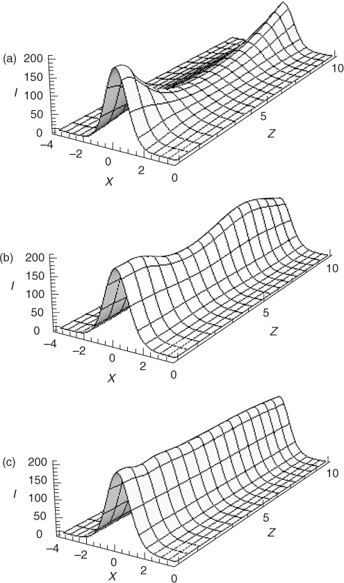
Figure 2.B.2 On-axis amplitude |u(0, 0, Z)| (normalized by |u(0, 0, 0)|) as a function of Z for the various inputs with different order perturbation. Dash-dot lines are for the zero-order perturbation, dashed lines for the first-order perturbation, solid lines for the second-order perturbation. From up to down, three perturbation cases with αd = 0.01, αd = 0.1, and αd = 0.2, respectively, and μ = 1.
The critical power for the first-order perturbation soliton is
2.B.6 ![]()
where ![]()
![]() , we take σ2 ≈ 2 and keep only the linear terms in a and b to obtain the expression of Pc, min. When θ0 = π/4, Pc reaches its minimum Pc, min, as shown in Figure 2.5b, which is the case of the first nematicon observed in experiments [73]. By making a = 0 and b = 0, we obtain the minimum critical power for the soliton with Gaussian profile
, we take σ2 ≈ 2 and keep only the linear terms in a and b to obtain the expression of Pc, min. When θ0 = π/4, Pc reaches its minimum Pc, min, as shown in Figure 2.5b, which is the case of the first nematicon observed in experiments [73]. By making a = 0 and b = 0, we obtain the minimum critical power for the soliton with Gaussian profile ![]() , which equals exactly the soliton power PS obtained in Reference 15 and the reference power
, which equals exactly the soliton power PS obtained in Reference 15 and the reference power ![]() given in Reference 14.9 To check the difference between Pc, min and
given in Reference 14.9 To check the difference between Pc, min and ![]() , we reexpress Pc, min and
, we reexpress Pc, min and ![]() with wFWHM and
with wFWHM and ![]() , respectively, and obtain
, respectively, and obtain
2.B.7 ![]()
where ![]() . Having
. Having ![]() , we obtain
, we obtain
2.B.8 ![]()
where ![]() . Therefore, we conclude that the relative error between Pc, min and
. Therefore, we conclude that the relative error between Pc, min and ![]() is as high as 50%, with Pc, min more precise than
is as high as 50%, with Pc, min more precise than ![]() .
.
Acknowledgments
This work was supported by the National Natural Science Foundation of China, Grant Nos.10474023, 10674050, 10804033, 10904041, 60908003, 61008007, 11074080.
The authors appreciate contributions from their coworker, Dr. Q. Shou, and all of their students involved in the recent work. One of the authors, Q. Guo, would like to thank Prof. Sien Chi of National Chiao Tung University (Taiwan, China) for valuable discussions at the beginning of this research.
Notes
1 Rigorously, the hypothesis of a time-harmonic electric field that has finite transverse cross section in space and is linearly polarized contradicts the law that an electric field must be divergence free in free space. The electric field, however, can be considered to be linearly polarized to the first-order approximation. For detail, see References 23–25.
2 Whether the “power” defined by Equation 2.6 is the actual power carried by the electromagnetic field depends on the dimensions of the function Ψ. If Ψ is scaled by a factor ( ε 0n0c/2)1/2 such that |Ψ|2 represents the optical intensity, Equation 2.6 gives the actual power; if Ψ represents the electric field with units V/m, the actual optical power is ![]() , as seen in Section 2.3. For the (1 + 1)-dimensional case (D = 1), the power
, as seen in Section 2.3. For the (1 + 1)-dimensional case (D = 1), the power ![]() is the power per unit length in the y direction.
is the power per unit length in the y direction.
3 The hypothesis here is an infinitely extended medium, necessary to guarantee linear momentum conservation. Boundary effects in a finite medium, which result in an oscillating soliton trajectory, are addressed in Chapter 11.
4 Here, we use the two terms optical breather and optical soliton to distinguish two states of nonlinear beam propagation. The breather and the soliton resemble a pair of twins born in several nonlinear physical systems. The breather [31, 32] is a localized solution that periodically oscillates versus propagation (in space or time), whereas the soliton is a localized solution that travels in propagation without changes in either shape or size. Although they are often referred to as optical solitons in most nonlinear optics literature, they are physically distinct: in the soliton, diffraction (or dispersion) is exactly balanced by nonlinearity, whereas in the breather [33, 34], diffraction (or dispersion) is only partly balanced by nonlinearity. In this sense, high order solitons of the nonlinear Schrödinger equation [22] should be referred to as optical breathers rather than optical solitons.
5 Snyder and Mitchell in Reference 5 pinpointed the evolution of the beam width, but not the phase evolution.
6 The model in Reference [53] (Equation 4 in the reference) is equivalent to an NNLSE (Eq. 2.4) with the response function R being the zeroth order modified Bessel function of the second kind; see Section 2.3.
7 Both results reported {the first of Equation 4 in Reference [62] and Equation 2 in Reference [64]} missed a factor 1/(2n0).
8 For the (1 + 1)-D case, one can have that P0 ∼ |Ψ(x, 0)|2w0 from the definition of “power,” P0 = ∫|Ψ(x, 0)|2dx and that ![]() because R(x) should be satisfied ∫R(x)dx = 1.
because R(x) should be satisfied ∫R(x)dx = 1.
9 In Reference 14, ![]() and
and ![]() . Then we can have
. Then we can have ![]() . Noting the equivalence of w0 to Rc, we obtain that
. Noting the equivalence of w0 to Rc, we obtain that ![]() .
.
1. G. I. Stegeman and M. Segev. Optical spatial solitons and their interactions: University and diversity. Science, 286:1518–1523, 1999.
2. G. I. Stegeman, D. N. Christodoulides, and M. Segev. Optical spatial solitons: Historical perspectives. IEEE J. Sel. Top. Quantum Electron., 6:1419–1427, 2000.
3. S. Trillo and W. Torruellas. Spatial Solitons. Springer-Verlag, Berlin, 2001.
4. Y. S. Kivshar and G. P. Agrawal. Optical Solitons: From Fibers to Photonic Crystals. Elsevier, New York, 2003.
5. A. W. Snyder and D. J. Mitchell. Accessible solitons. Science, 276:1538–1541, 1997.
6. G. Assanto, et al. Nematicons. Opt. Photon. News, 14:45–48, 2003; Spatial solitons in nematic liquid crystals. IEEE J. Quantum Electron., 39:13–21, 2003; Routing light at will, J. Nonlin. Opt. Phys. Mater., 6:37–47, 2007; Nematicons: Self-localized beams in nematic liquid crystals, Liq. Cryst., 36:1161–1172, 2009.
7. W. Królikowski, O. Bang, N. I. Nikolov, D. Neshev, J. Wyller, J. J. Rasmussen and D. Edmundson. Modulational instability, solitons and beam propagation in spatially nonlocal nonlinear media. J. Opt. B: Quantum Semiclass. Opt., 6:288–294, 2004.
8. Q. Guo. Nonlocal spatial solitons and their interactions, Proceedings on Optical Transmission, Switching, and Subsystems, eds. C. F. Lam, C. Fan, N. Hanik, and K. Oguchi. Proceedings of SPIE (Asia-Pacific Optical and Wireless Communications Conference, November 2–6, Wuhan, P.R.China 2003). 5281: 581–594, 2004.
9. D. J. Mitchell and A. W. Snyder. Soliton dynamics in a nonlocal medium. J. Opt. Soc. Am. B, 16:236–239, 1999.
10. W. Królikowski, O. Bang, J. J. Rasmussen, and J. Wyller. Modulational instability in nonlocal nonlinear Kerr media. Phys. Rev. E, 64:016612, 2001.
11. W. Królikowski and O. Bang. Solitons in nonlocal nonlinear media: Exact solutions. Phys. Rev. E, 63:016610, 2001.
12. O. Bang, W. Królikowski, J. Wyller, and J. J. Rasmussen. Collapse arrest and soliton stabilization in nonlocal nonlinear media. Phys. Rev. E, 66:046619, 2002.
13. Y. R. Shen. Solitons made simple. Science, 276:1520–1520, 1997.
14. C. Conti, M. Peccianti, and G. Assanto. Route to nonlocality and observation of accessible solitons. Phys. Rev. Lett., 91:073901, 2003.
15. C. Conti, M. Peccianti, and G. Assanto. Observation of optical spatial solitons in highly nonlocal medium. Phys. Rev. Lett., 94:113902, 2004.
16. C. Rotschild, O. Cohen, O. Manela, M. Segev, and T. Carmon. Solitons in nonlinear media with an infinite range of nonlocality: First observation of coherent elliptic solitons and of vortex-ring solitons. Phys. Rev. Lett., 95:213904, 2005.
17. A. Dreischuh, D. Neshev, D. E. Peterson, O. Bang, and W. Królikowski, Observation of attraction between dark soliton. Phys. Rev. Lett., 96:043901, 2006.
18. S. Skupin, M. Saffman, and W. Królikowski. Nonlocal stabilization of nonlinear beams in a self-focusing atomic vapor. Phys. Rev. Lett., 98:263902, 2007.
19. C. Conti, A. Fratalocchi, M. Peccianti, G. Ruocco, and S. Trillo. Observation of a gradient catastrophe generating solitons. Phys. Rev. Lett., 102:083902, 2009.
20. R. W. Boyd. Nonlinear Optics, 3rd edn, Chapters 4–5 and 7. Academic Press, Amsterdam, 2008.
21. Y. R. Shen. The Principles Of Nonlinear Optics, Chapter 16. John Wiley & Sons, New York, 1984.
22. G. P. Agrawal. Nonlinear Fiber Optics, 3rd edn. Academic Press, San Diego, CA, 2001.
23. M. Lax, W. H. Louisell, and W. B. McKnight. From Maxwell to paraxial wave optics. Phys. Rev. A, 11:1365–1370, 1975.
24. S. Chi and Q. Guo. Vector theory of self-focusing of an optical beam in Kerr media. Opt. Lett., 20:1598–1600, 1995.
25. H. A. Haus. Waves and Fields in Optoelectronics, Chapter 4. Prentice-Hall, New Jersey, 1984.
26. I. N. Bronshtein and K. A. Semendyayev. Handbook of Mathematics, 4.2.2.9, Leipzig, 539, 1985.
27. A. I. Yakimenko, V. M. Lashkin, and O. O. Prikhodko. Dynamics of two-dimensional coherent structures in nonlocal nonlinear media. Phys. Rev. E, 73:066605, 2006.
28. S. Ouyang, W. Hu, and Q. Guo. Light steering in strongly nonlocal nonlinear medium. Phys. Rev. A, 76:053832, 2007
29. W. Hu, S. Ouyang, P. Yang, Q. Guo, and S. Lan. Short-range interactions between strongly nonlocal spatial solitons. Phys. Rev. A, 77:033842, 2008.
30. Q. Guo, B. Luo, F. Yi, S. Chi, and Y. Xie. Large phase shift of nonlocal optical spatial solitons. Phys. Rev. E, 69:016602, 2004.
31. G. L. Lamb Jr. Elements of Soliton Theory, Chapter 5. John Wiley & Sons, New York, 133–168, 1980.
32. S. Flach and C. R. Willis. Discrete breathers. Phys. Rep., 295:181–264, 1998.
33. R. Michalska-Trautman. Formation of an optical breather. J. Opt. Soc. Am. B, 6:36–44, 1989.
34. J. N. Kutz, P. Holmes, S. G. Evangelides Jr., and J. P. Gordon. Hamiltonian dynamics of dispersion-managed breathers. J. Opt. Soc. Am. B, 15:87–96, 1998.
35. Q. Shou, X. Zhang, W. Hu, and Q. Guo. Large phase shift of spatial solitons in lead glass. Opt. Lett., 36:4194–4196, 2011.
36. Q. Guo, B. Luo, and S. Chi. Optical beams in sub-strongly non-local nonlinear media: A variational solution. Opt. Commun., 259:336–341, 2006.
37. S. Ouyang, Q. Guo, and W. Hu. Perturbative analysis of generally nonlocal spatial optical solitons. Phys. Rev. E, 74:036622, 2006.
38. X. Zhang and Q. Guo. Analytical solution in the Hermite-Gaussian form of the beam propagating in the strong nonlocal media. Acta. Phys. Sin., 54:3178–3182, 2005 (in Chinese).
39. D. Deng, X. Zhao, Q. Guo, and S. Lan. Hermite-Gaussian breathers and solitons in strongly nonlocal nonlinear media. J. Opt. Soc. Am. B, 24:2537–2544, 2007.
40. X. Zhang, Q. Guo, and W. Hu. Analytical solution to the spatial optical solitons propagating in the strong nonlocal media. Acta. Phys. Sin., 54:5189–5193, 2005 (in Chinese).
41. D. Deng and Q. Guo. Propagation of Laguerre-Gaussian beams in nonlocal nonlinear media. J. Opt. A.: Pure Appl. Opt., 10:035101, 2008.
42. W. Zhong and Y. Lin. Two-dimensional Laguerre-Gaussian soliton family in strongly nonlocal nonlinear media. Phys. Rev. A, 75:061801, 2007.
43. D. Deng and Q. Guo. Ince-Gaussian solitons in strongly nonlocal nonlinear media. Opt. Lett., 32:3206–3208, 2007.
44. D. Deng and Q. Guo. Ince-Gaussian beams in strongly nonlocal nonlinear media. J. Phys. B: At. Mol. Opt., 41:145401, 2008.
45. D. Deng, Q. Guo, and W. Hu. Hermite-Laguerre-Gaussian beams in strongly nonlocal nonlinear media. J. Phys. B: At. Mol. Opt., 41:225402, 2008.
46. D. Briedis, D. E. Petersen, D. Edmundson, W. Królikowski, and O. Bang. Ring vortex solitons in nonlocal nonlinear media. Opt. Express, 13:435–443, 2005.
47. D. Buccoliero, A. S. Desyatnikov, W. Królikowski, and Y. S. Kivshar. Laguerre and Hermite soliton clusters in nonlocal nonlinear media. Phys. Rev. Lett., 98:053901, 2007.
48. D. Buccoliero, A. S. Desyatnikov, W. Królikowski, and Y. S. Kivshar. Spiraling multivortex solitons in nonlocal nonlinear media. Opt. Lett., 33:198–200, 2008.
49. D. Buccoliero and A. S. Desyatnikov. Quasi-periodic transformations of nonlocal spatial solitons. Opt. Express, 17:9608–9613, 2009.
50. D. W. McLaughlin, D. J. Muraki, and M. J. Shelley. Self-focused optical structures in a nematic liquid crystal. Physica D, 97:471–497, 1996.
51. Z. Xu, Y. V. Kartashov, and L. Torner. Upper threshold for stability of multipole-mode solitons in nonlocal nonlinear media. Opt. Lett., 30:3171–3173, 2005.
52. L. Dong and F. Ye. Stability of multipole-mode solitons in thermal nonlinear media. Phys. Rev. A, 81:013815, 2010.
53. A. I. Yakimenko, Y. A. Zaliznyak, and Y. S. Kivshar. Stable vortex solitons in nonlocal self-focusing nonlinear media. Phys. Rev. E, 71:065603, 2005.
54. C. Rotschild, M. Segev, Z. Xu, Y. V. Kartashov, L. Torner, and O. Cohen. Two-dimensional multipole solitons in nonlocal nonlinear media. Opt. Lett., 31:3312–3314, 2006.
55. S. Skupin, O. Bang, D. Edmundson, and W. Królikowski. Stability of two-dimensional spatial solitons in nonlocal nonlinear media. Phys. Rev. E, 73:066603, 2006.
56. D. Deng, Q. Guo, and W. Hu. Complex-variable-function Gaussian solitons. Opt. Lett., 34:43–45, 2009.
57. D. Deng, Q. Guo, and W. Hu. Complex-variable-function Gaussian beam in strongly nonlocal nonlinear media. Phys. Rev. A, 79:023803, 2009.
58. S. Lopez-Aguayo, A. S. Desyatnikov, and Y. S. Kivshar. Azimuthons in nonlocal nonlinear media. Opt. Express, 14:7903–7908, 2006.
59. D. Mendlovic and H. M. Ozaktas. Fractional Fourier transforms and their optical implementation. J. Opt. Soc. Am. A, 10:1875–1881, 1993.
60. D. Lu, W. Hu, Y. Zheng, Y. Liang, L. Cao, S. Lan, and Q. Guo. Self-induced fractional Fourier transform and revivable higher-order spatial solitons in strongly nonlocal nonlinear media. Phys. Rev. A, 78:043815, 2008.
61. V. Namias. The fractional order Fourier transform and its application to quantum mechanics. J. Inst. Math. Appl., 25:241–265, 1980.
62. M. Peccianti, C. Conti, and G. Assanto. Interplay between nonlocality and nonlinearity in nematic liquid crystals. Opt. Lett., 30:415–417, 2005.
63. W. Hu, T. Zhang, Q. Guo, L. Xuan, and S. Lan. Nonlocality-controlled interaction of spatial solitons in nematic liquid crystals. Appl. Phys. Lett., 89:071111, 2006.
64. L. Cao, Y. Zheng, W. Hu, and Q. Guo. Long-range interactions between nematicons. Chin. Phys. Lett., 26:064209, 2009.
65. P. D. Rasmussen, O. Bang, and W. Królikowski. Theory of nonlocal soliton interaction in nematic liquid crystals. Phys. Rev. E, 72:066611, 2005.
66. M. Peccianti, C. Conti, G. Assanto, A. De Luca, and C. Umeton. Nonlocal optical propagation in nonlinear nematic liquid crystals. J. Nonlin. Opt. Phys. Mater., 12:525–538, 2003.
67. H. Ren, S. Ouyang, Q. Guo, and L. Wu. (1 + 2)-Dimensional sub-strongly nonlocal spatial optical solitons: perturbation method. Opt. Commun., 275:245–251, 2007.
68. S. Ouyang and Q. Guo. (1 + 2)-dimensional strongly nonlocal solitons. Phys. Rev. A, 76:053833, 2007.
69. H. Ren, S. Ouyang, Q. Guo, W. Hu, and L. Cao. A perturbed (1 + 2)-Dimensional soliton solution in nematic liquid crystals. J. Opt. A: Pure Appl. Opt., 10:025102, 2008.
70. M. Peccianti, K. A. Brzdakiewicz, and G. Assanto. Nonlocal spatial soliton interactions in bulk nematic liquid crystals. Opt. Lett., 27:1460–1462, 2002.
71. Y. Xie and Q. Guo. Phase modulations due to collisions of beam pairs in nonlocal nonlinear media. Opt. Quantum Electron., 36:1335–1351, 2004.
72. C. Rotschild, B. Alfassi, O. Cohen, and M. Segev. Long-range interactions between optical solitons. Nat. Phys., 2:769–774, 2006.
73. M. Peccianti, A. De Rossi, G. Assanto, A. De Luca, C. Umeton, and I. C. Khoo. Electrically assisted self-confinement and waveguiding in planar nematic liquid crystal cells. Appl. Phys. Lett., 77:7–9, 2000.