
Chapter 7: Interaction of Nematicons and Nematicon Clusters
Department of Mathematics and Mechanics, IIMAS, Fenomenos Nonlineales y Mecánica, Universidad Nacional Autónoma de México, Mexico D.F., Mexico
School of Mathematics and Maxwell Institute for Mathematical Sciences, University of Edinburgh, Edinburgh, Scotland, United Kingdom
7.1 Introduction
The theory for modeling and evolution of a single solitary wave in a nematic liquid crystal, a nematicon, has been described in Chapter 3. One of the key concepts discussed in that chapter was that of the nonlocal response of the nematic medium. This nonlocal response means that the perturbation due to the optical beam on the nematic extends far beyond the waist of the optical beam itself. Although an important effect for a single nematicon, it stops the catastrophic collapse that occurs in the case of a local two-dimensional optical solitary wave [1], it becomes vital when the interaction of multiple nematicons is studied. The nonlocal perturbation of the nematic means that two optical beams can interact through the nematic even though they appear to be well separated. Indeed, the interaction between two or more nematicons will be found to have a close connection with the action at a distance of Newtonian gravitation [2].
A primary motivation for the study of the interaction of nematicons is that this interaction can be used as the basis for all-optical routing and logic devices based on nematic liquid crystals [3–7]. The fundamental concept is that the trajectory of a signal beam can be altered by the presence of a control beam, or control beams, resulting in the signal beam being routed to a given output. This control is both through the relative physical positions of the control beams and their powers. The detailed understanding of the interaction of nematicons, particularly their interaction via the nematic, is therefore vital for the development of all-optical devices based on nonlinear beams in nematic liquid crystals. These potential applications, as well as intrinsic interest, have motivated a great deal of study of the interaction of nematicons propagating in the same direction [8–13] and counterpropagating nematicons [14–16].
All proposed logic devices are based on the adjustable routing of a signal beam from a given input to a range of possible outputs at the other end of the liquid crystal cell. The advantage of a liquid crystal as the intermediary medium is that there are no fixed “circuits,” unlike a wire-based device, so that any path through the cell is possible. This reconfigurable flexibility of a liquid-crystal-based logic device is potentially a great advantage. There are two basic mechanisms for optically controlling the trajectory of a signal beam in a liquid crystal cell. The first involves the interaction of two nematicon beams [3, 6, 8–10, 12]. The strength of the interaction between two or more nematicons depends on both their relative separation and their optical power, with stronger interaction occurring at closer separation and higher power. In the case of solitary waves for local nonlinear Schrödinger-type (NLS-type) equations
7.1 ![]()
the interaction between solitary waves depends not only on their separation and power but also on their relative phase [1]. If the solitary waves are in phase, then they attract and if they are π out of phase, they repel [1]. For other phase differences, the interaction is more complicated [1]. In the case of nonlocal media, such as liquid crystals, there is the added effect of attraction due to the medium-mediated mutual interaction. This nonlocal interaction can be sufficient to overcome the repulsion of out of phase solitary waves [8–12, 17]. When the solitary waves have angular momentum, stable rotating bound vector solitary waves can result [9–12, 17]. Therefore, in experimental situations, the phase difference between the nematicons plays no role in the switching properties of the proposed logic devices. There are a number of ways in which switching can be realized. The output point of a signal beam can be controlled by the absence or presence of a control beam. Multiple beams can be routed to different outputs, depending on the presence or absence of other beams and the strength of the mutual interaction. In this manner, elementary logic can be performed whereby the output point of a given signal depends on the properties of other signals.
A second type of beam interaction scenario involves nematicons interacting with localized beams propagating in a direction orthogonal to the nematicon [5, 4, 7]. In this case, these orthogonal beams form a localized refractive index change, which alters the nematicon trajectory when it passes close to the beam. This is similar to the familiar refraction of light, except in this case the refractive index change has a nonlinear dependence on the beam power. Again, the absence or presence of the control beam can switch the nematicon between different outputs. An additional benefit of using control beams is that it is easy to introduce multiple beams in a cell, resulting in complicated nematicon trajectories. By actually passing a nematicon through the orthogonal control beam, it is possible to split the nematicon, resulting in a Y junction [5].
This discussion of potential applications of nematicons in all-optical logic and signal processing devices shows the importance of a detailed understanding of the interaction of multiple nematicons. This topic is discussed in detail in the following sections.
7.2 Gravitation of Nematicons
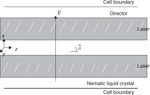
The simplest configuration in which to consider the interaction of nematicons is that of so-called two-color nematicons. In this configuration, the two nematicons are based on polarized beams of two different wavelengths (colors). The mathematical analysis of the incoherent interaction of two nematicons is much easier than that of coherent interaction. This is because in the case of coherent interaction the nematicons interact directly [17], whereas in the case of incoherent interaction they only interact through the nematic. This results in far fewer terms in the resulting modulation equations and a far clearer picture of the interaction. The detailed setup of the liquid crystal cell is as for a single nematicon and is illustrated in Figure 7.1. A static electric field is applied in the x direction to overcome the , so that in the absence of light the optical director is pretilted at an angle ![]() to the z direction. The angle θ will then measure the perturbation of the director angle from this pretilt due to the optical beams. In nondimensional form, the equations governing the propagation of the two color beams in the cell are
to the z direction. The angle θ will then measure the perturbation of the director angle from this pretilt due to the optical beams. In nondimensional form, the equations governing the propagation of the two color beams in the cell are
see Alberucci et al. [19]. Here, u and v are the slowly varying envelopes of the electric fields of the two beams. The Laplacian ∇2 is in the (x,y) plane. The coefficients Du and Dv are the diffraction coefficients for the two colors and Au and Av are the coupling coefficients between the light and the nematic for the two colors. The parameter ν measures the elasticity of the nematic and q is related to the square of the static electric field that pretilts the nematic [20–22]. These two-color nematicon equations have the Lagrangian formulation
where the superscript * denotes the complex conjugate. The nematicon equations (Eqs 7.2, 7.3, 7.4) show that the nematicons interact only via the director (Eq. 7.4) and not via direct beam on beam interaction [17]. The incoherent interaction of nematicons of the same color is also governed by the system (Eqs 7.2, 7.3, 7.4), with Du = Dv and Au = Av.
Figure 7.1 Liquid crystal cell with two polarized light beams of different colors. is the pretilt angle due to the electric field E in the x direction. (Source: Reproduced with permission from Figure 7.1 in Reference 18.)
The evolution of the two-color nematicons, governed by Equations 7.2, 7.3, 7.4, will be analyzed using the averaged Lagrangian method discussed in Chapter 3. To this end, the profiles of the two nematicons will be assumed to be given by the trial functions
where
7.7 
At this stage, the actual detailed functional form f(ζ) of the nematicons will not be specified. Indeed, in many interaction scenarios involving nematicon interactions in liquid crystals, the trajectories of the nematicons are essentially independent of the transverse profile of the nematicon [2, 18, 23, 24]. In the present chapter, both hyperbolic secant f(ζ) = sech ζ and Gaussian f(ζ) = exp( − ζ2) profiles are used as examples.
Substituting the trial functions (Eq. 7.6) into the Lagrangian (Eq. 7.5) and averaging by integrating in x and y from − ∞ to ∞ yield, as explained in detail in Chapter 3, the averaged Lagrangian
The interaction component of the averaged Lagrangian is
7.9 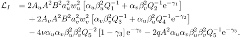
Here,
7.10 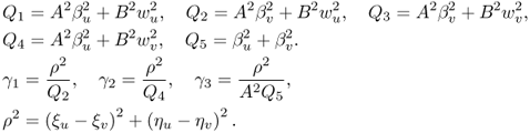
The areas, modulo 2π, of the shelves of radiation under the nematicons are
7.11 ![]()
The variable ρ is the distance between the two nematicons and will be found to be analogous to the distance between masses in Newtonian gravitation. Taking variations of the averaged Lagrangian (Eq. 7.8) results in the modulation equations
plus the algebraic equations
![]()
together with symmetric equations in the v color, for the evolution of the parameters of the two-color nematicons. Equation 7.12 is the equation of conservation of mass in the sense of scale invariances of the Lagrangian (Eq. 7.5) [25]. Although it physically corresponds to conservation of mass in the application of the NLS equation to water waves, in the present optical context it corresponds to conservation of power, or equivalently, photon number.
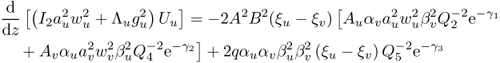
The modulation Equations 7.17 and 7.18 are x and y momentum equations for the color u. The equations for total momentum conservation in the x and y directions can then be obtained by adding the momentum Equations 7.17 and 7.18 to their v color counterparts, to give total x momentum conservation as
7.21 ![]()
and total y momentum conservation as
7.22 ![]()
That these are, in fact, x and y momentum conservation equations can be verified by the application of Nöther's theorem to the Lagrangian (Eq. 7.5) based on invariances to shifts in the space directions x and y [26].
The modulation Equations 7.12, 7.13, 7.14, 7.15, 7.16, 7.17, 7.18, 7.19, 7.20 and their symmetric v counterparts can be put in a simpler form using Kepler coordinates. Let us define the vector position of the u color nematicon by ξu = (ξu, ηu) and that of the v color nematicon by ξv = (ξv, ηv). The relative displacement of the nematicons, defined by Equation 7.10, in vector form, is
7.23 ![]()
The “mass” conservation equation (Eq. 7.12) shows that the “masses” of the u and v color nematicons can be defined to be
The center of “mass” of the two nematicons can then be defined to be
It should be noted that the masses of the nematicons have been weighted by the diffraction coefficients in this definition of the center of mass. These weightings, other than being a mere analogy with Newtonian gravitation, reflect the different linear optical propagation of the two beams. Relative to the center of mass (Eq. 7.25), polar coordinates will be defined based on ρ and the polar angle denoted by ϕ, similar to the case of the Kepler problem. In a similar manner to the gravitational problem, the equations for the positions of the two-color nematicons can then be shown to be the conservation of angular momentum equation
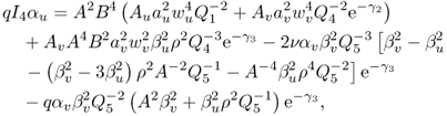
where L is the constant angular momentum, and the radial equations
and
The potential Φ, which can be found from the averaged Lagrangian (Eq. 7.8) using a point transformation to calculate the corresponding averaged Hamiltonian, is
7.29 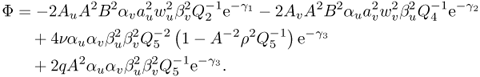
These dynamical equations for the positions of the nematicons are the same as those for two masses in Newtonian gravitation [27], except that the potential is not the inverse separation potential of Newton's law of gravitation. In addition, the potential (Eq. 7.29) is nonmonotonic and so there exist multiple steady states for the separation of the nematicons [28], unlike the unique steady state for gravitation. The center of mass equation (Eq. 7.27) is just a statement of conservation of linear momentum.
The gravitational forms (Eqs 7.26, 7.27, 7.28) of the modulation equations for the two-color nematicons have an obvious extension to n-color interacting nematicons [29].
7.3 In-Plane Interaction of Two-Color Nematicons
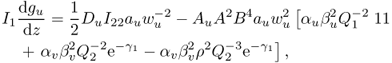
Let us consider the interaction of two-color nematicons in the nonlocal limit, so that the nonlocality parameter ν is large. Typical experimental values of ν are O(100) [30]. As the nematicons propagate over a large z distance they evolve to a steady state by shedding diffractive radiation. Hence, loss to shed diffractive radiation must be included in the modulation equations of Section 7.2 [22, 31, 32]. The largest effect on the nematicons of this loss to shed diffractive radiation is the loss of mass, or optical power in this context [22, 32, 33]. The momentum and energy shed in diffractive radiation is of higher order than the shed mass [33]. The mass conservation equation (Eq. 7.12) and its v color counterpart will then need to be modified to incorporate this loss. Furthermore, as the shelves of low wave number radiation under the nematicons must link to the shed radiation, Equation 7.15 for gu and the equation for its v color counterpart gv must also be modified. The details of this modification are given in Kath and Smyth [33], García-Reimbert et al. [34], Minzoni et al. [32], and in Chapter 3 and so will not be repeated here. The final result is that loss terms are added to the mass Equation 7.12 and Equation 7.15 for gu, so that they become
7.30 ![]()
and
7.31 
In these equations, the loss coefficient δu is
Finally,
7.33 ![]()
where
7.34![]()
The mass equation in the v color and the equation for gv are modified in a similar manner to incorporate loss. In the expression (Eq. 7.33) for κu the ![]() superscript denotes fixed point values.
superscript denotes fixed point values.
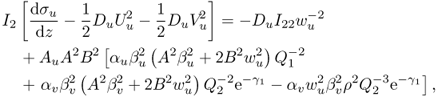
The final steady nematicon state is found from the equation for total energy conservation for the nematicon equations (Eqs 7.2, 7.3, 7.4). This energy conservation equation is most easily found using Nöther's theorem based on the invariance of the Lagrangian (Eq. 7.5) to shifts in z [26]. In this manner, we find that the conserved energy density is
Averaging this conserved energy density by integrating in x and y from − ∞ to ∞ yields the energy conservation modulation equation
The modulation equation (Eq. 7.15), together with its v color counterpart, give the fixed point relations between âu and ![]() u and âv and
u and âv and ![]() v. With these relations, the energy conservation equation (Eq. 7.36) then gives the fixed point amplitudes and widths from the known initial beams.
v. With these relations, the energy conservation equation (Eq. 7.36) then gives the fixed point amplitudes and widths from the known initial beams.
Figure 7.2 Comparisons between full numerical and modulation solutions for the initial values au = av = 1.8, wu = wv = 3.0, ξu = 1.0, ξv = − 1.0, Uu = − 0.1, Uv = − 0.05, Vu = Vv = 0, ηu = ηv = 0 with ν = 500, q = 2, Au = 1.0, Av = 0.95, Du = 1.0, Dv = 0.98. f(ζ) = sech ζ. Solid line: full numerical solution u; dot-dashed line: full numerical solution v; dotted line: solution of modulation equations for u; dashed line: solution of modulation equations for v. (a) Positions; (b) amplitudes. Reproduced with permission from Figure 7.2 in Reference 31.
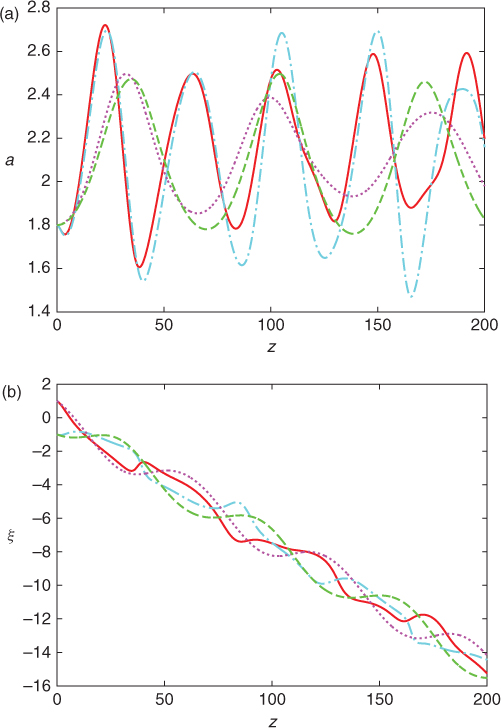
Figure 7.2 shows a comparison of the amplitudes and positions of the nematicons as given by the full numerical solution of the nematicon equations (Eqs 7.2, 7.3, 7.4) and the solution of the modulation equations with loss to diffractive radiation for a typical set of initial conditions. For this set of initial conditions the nematicons are initially moving in the same direction. The nematicons oscillate about each other following a mean trajectory as they evolve. This mean trajectory is given by conservation of linear momentum and is the center of mass position (Eq. 7.25), as is discussed later. There is excellent agreement in the positions of the nematicons, with a slight disagreement in the periods of the position oscillations for larger values of z. The agreement between the amplitudes is not so good. The numerical amplitude evolution shows much more complicated behavior than that given by the modulation equations, which shows smooth oscillations that decay in amplitude owing to radiation loss. As the amplitude-width evolutions of the nematicons form nonlinear oscillators, the differences in the amplitudes of the oscillations as given by the numerical and modulation solutions translate into period differences.
Figure 7.3 Comparisons between full numerical and modulation solutions for the initial values au = av = 1.8, wu = wv = 3.0, ξu = 1.0, ξv = − 1.0, Uu = − 0.1, Uv = 0.05, Vu = Vv = 0, and ηu = ηv = 0, with ν = 500, q = 2, Au = 1.0, Av = 0.95, Du = 1.0, Dv = 0.98. f(ζ) = sech ζ. Solid line: full numerical solution u; dot-dashed line: full numerical solution v; dotted line: solution of modulation equations for u; dashed line: solution of modulation equations for v. (a) Positions; (b) amplitudes.
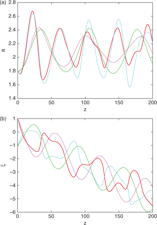
Figure 7.4 Full numerical solution for |u| at z = 100 and y = 0 for the initial values au = av = 1.2, wu = wv = 4.0, ξu = 1.0, ξv = − 1.0, Uu = 0.1, Uv = − 0.05, Vu = Vv = 0, and ηu = ηv = 0, with q = 2, Au = 1.0, Av = 0.95, Du = 1.0, Dv = 0.98. f(ζ) = sech ζ. Solid line: solution for ν = 250; dashed line: solution for ν = 500; and dotted line: solution for ν = 1000. (Source: Reproduced with permission from Figure 7.3 in Reference 31.)
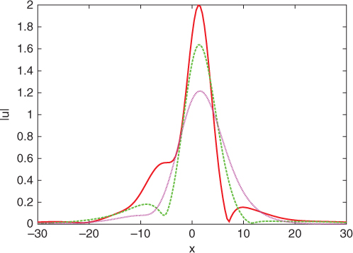
Figure 7.3 shows similar comparisons between the full numerical and modulation solutions for an initial condition for which the nematicons initially move in opposite directions. In this case the total linear momentum is less, so that the mean speed of the nematicons is not as large. The position comparison is again excellent, with a slight period difference for large z. The numerical amplitude again shows more complicated behavior and is more complicated than the evolution shown in Figure 7.3a. The reason for this more complicated amplitude evolution as shown by the full numerical solution is discussed in the following text.
Figure 7.5 Steady value ![]() as a function of Uv0 for the initial values au = av = 1.8, wu = wv = 3.0, ξu = 1.0, ξv = − 1.0, and Uu = 0.1 with ν = 500, q = 2, Au = 1.0, Av = 0.95, Du = 1.0, Dv = 0.98. f(ζ) = sech ζ. Crosses: full numerical solution; dashed line: solution of modulation equations; dotted line: momentum conservation result. (Source: Reproduced with permission from Figure 7.4 in Reference 31.)
as a function of Uv0 for the initial values au = av = 1.8, wu = wv = 3.0, ξu = 1.0, ξv = − 1.0, and Uu = 0.1 with ν = 500, q = 2, Au = 1.0, Av = 0.95, Du = 1.0, Dv = 0.98. f(ζ) = sech ζ. Crosses: full numerical solution; dashed line: solution of modulation equations; dotted line: momentum conservation result. (Source: Reproduced with permission from Figure 7.4 in Reference 31.)
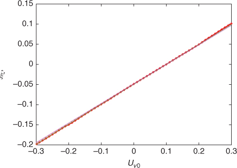
Figure 7.4 shows the profile |u| of the u color beam at a fixed value of z for various values of the nonlocality parameter ν. It can be seen that the interaction of the beam with the beam in the v color has resulted in a significant distortion of its profile, particularly for values of v in the experimental range O(100). In addition, the shelves of radiation extending out from the beam show distortion. As the nonlocality parameter ν increases, the beam distortion decreases. The reason for this distortion of the beam shape is clear. The beam is being accelerated by its interaction with the v color beam and does not undergo symmetric interaction over its profile. This introduces asymmetry in the interaction, which deforms the profile. These changes in profile are, of course, not taken into account by the fixed trial functions (Eq. 7.6). Indeed, it is not obvious how to introduce realistic beam distortions into the trial functions. The beam positions are not greatly affected by the beam distortions as the trajectories are determined by the linear momentum of the beams, which depends on the total mass (optical power), an integral quantity not sensitive to the details of the beam profile. Fixed trial functions can then give good results for the beam trajectories.
The Kepler-like modulation equations of Section 7.2 predict that the nematicons will orbit about each other, much as for two gravitating bodies. However, when loss to shed diffractive radiation is included, the nematicons can spiral into each other and form a bound state propagating at the same position. For nematicons propagating in the plane with no angular momentum, this shedding of radiation will always result in a bound state as long as their initial linear momentum difference is not too large. When the nematicons have angular momentum, the situation is more complicated. As the nematicons shed radiation they lose angular momentum. There exists a threshold angular momentum at which there is a cutoff in angular momentum shed to radiation in the form of spiral waves [29]. This cutoff means that a stable bound state of orbiting two-color nematicons can form even though there is loss to diffractive radiation.
Let us then consider in-plane nematicon interaction, in the x plane say, resulting in a bound state of copropagating nematicons. If linear momentum loss to shed diffractive radiation is neglected, the x linear momentum conservation equation (Eq. 7.21) and the trajectory equation (Eq. 7.14) and their v color counterparts show that the position of this copropagating bound state is given by
where the initial x linear momentum is
7.38 ![]()
Here, the 0 subscripts refer to initial values of the quantities. Figure 7.5 shows a comparison between ![]() as given by the full numerical solution of the two-color nematicon equations (Eqs 7.2, 7.3, 7.4), the solution of the modulation equations with radiative loss, and the momentum conservation result (Eq. 7.37). It can be seen that there is excellent agreement between the numerical and modulation solutions. Furthermore, the momentum conservation result (Eq. 7.37), which ignores momentum shed in diffractive radiation, gives an excellent prediction for
as given by the full numerical solution of the two-color nematicon equations (Eqs 7.2, 7.3, 7.4), the solution of the modulation equations with radiative loss, and the momentum conservation result (Eq. 7.37). It can be seen that there is excellent agreement between the numerical and modulation solutions. Furthermore, the momentum conservation result (Eq. 7.37), which ignores momentum shed in diffractive radiation, gives an excellent prediction for ![]() . This excellent agreement shows that in the nonlocal limit there is little momentum shed in diffractive radiation, unlike in the local limit [18]. This conforms with the general trend that as the nonlocality ν increases, the rate of loss to diffractive radiation decreases and it takes longer for nematicons to evolve to the steady state.
. This excellent agreement shows that in the nonlocal limit there is little momentum shed in diffractive radiation, unlike in the local limit [18]. This conforms with the general trend that as the nonlocality ν increases, the rate of loss to diffractive radiation decreases and it takes longer for nematicons to evolve to the steady state.
7.4 Multidimensional Clusters
The analogy of nematicon motion with the gravitational Kepler problem, explored in Section 7.2, suggests that other configurations known from classical mechanics could have equivalents in nematicon motion in liquid crystals, examples being the Lagrange triangle solution and figure of 8 solution from Newtonian gravitation [35] and cluster solutions, which include large bodies surrounded by smaller bodies rotating in a synchronized manner, similar to that which occurs with Saturn and its rings. It needs to be emphasized that the experimental verification of such configurations may not be easy, at least for current liquid crystal types, owing to scattering and other losses in the liquid crystal, which become more important when several beams impinge on the same cell. However, it is of interest to examine the similarities and differences between the nematicon case and the equivalent Newtonian gravitation configurations. The differences are due to the nonmonotonic nature of the interaction potential between nematic beams, as shown by the potential (Eq. 7.29), and, to a lesser extent, by the deformable, nonrigid nature of nematicons, in contrast to gravitating masses. In particular, the diffractive radiation shed by the nematic beams as they move about a common center can cause the ultimate merging or collapse of the multinematicon cluster. In this section, we describe some of the analysis of Simon [35] for the gravitational Lagrange triangular three-body solution and its extension to three interacting nematicons and perform a numerical examination of the effect of a vortex on a cluster of two rotating nematicons.
Let us begin by considering the analog of the Lagrange triangle solution of Newtonian gravitation [35] for three nematicons of three different colors (wavelengths) [29]. In the gravitational case, the homogeneity of the potential, together with its monotonicity, results in rigidly rotating masses with the masses at the vertices of an equilateral triangle. Moreover, in the limit in which one of the masses is much larger than the other two, this gravitation triangle configuration is linearly stable [35]. This linear stability becomes apparent when the triangle configuration is treated as two decoupled two-body Kepler problems for which the small masses rotate around the large one, keeping the triangle configuration. A natural analogy is then the evolution of three nematicons of different colors (wavelengths). These evolve according to the equations [19, 29]
7.40 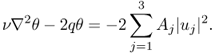
Here, Dj and Aj are the diffraction coefficients and coupling coefficients for the three colors, respectively. Let us consider initial conditions of the form
7.41 ![]()
where
The peaks (ξj, ηj) of the nematicons are placed at the vertices of a triangle. The velocities (Uj, Vj) are chosen to be approximately orthogonal to the position vectors of the peaks from the center of the triangle to ensure rotation about this center.
Figure 7.6 shows an example of an unstable three-color nematicon cluster. This example shows a typical instability whereby two of the nematicons lock and the third one escapes. The two locked nematicons orbit each other as for the two-color-coupled nematicons of Section 7.3.
Figure 7.6 Numerical positions (x,y) of three nematicons up to z = 200. u1: solid line; u2: dashed line; u3: dotted line. The initial conditions are ![]() with q = 10, ν = 50, D1 = 1.0, D2 = 0.95, D3 = 0.98, A1 = 1.0, A2 = 0.9 and A3 = 0.95.
with q = 10, ν = 50, D1 = 1.0, D2 = 0.95, D3 = 0.98, A1 = 1.0, A2 = 0.9 and A3 = 0.95.
To gain an understanding of the dynamics of three-color nematicon clusters, let us develop a modulation theory based on the trial functions
7.43 
for the nematicons and the director response [32, 33]. Here,
7.44 ![]()
and all the parameters in the trial functions depend on the distance z down the cell. The three-color nematicon equations (Eqs 7.39 and 7.40) have the Lagrangian
Substituting the trial functions (Eq. 7.43) into this Lagrangian and integrating x and y over the whole plane, − ∞ < x, y < ∞, that is averaging, result in the averaged Lagrangian
with the various integrals Ii and Iij given in Appendix 7.A. From the potential (Eq. 7.29), the interaction potential Φij of the nematicons is
7.47 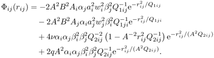
The separation of the nematicons is
7.48 ![]()
Finally, the quantities Q1ij and Q2ij appearing in the averaged Lagrangian are
Taking variations of the averaged Lagrangian (Eq. 7.46) with respect to the parameters gives the equations governing the evolution and positions of the nematicons. As in Section 7.2, the equations for the positions ξi = (ξi, ηi) of the nematicons can be put in the classical mechanics form
where the mass, or optical power, of a nematicon is
However, to derive the three-color Lagrange solution and study its stability, it is more convenient to use the coordinate system sketched in Figure 7.7 [35]. In this coordinate system, the motion of the center of mass of the nematicons is decoupled from their relative motion. In this coordinate system, equations (Eq. 7.50) for the positions of the nematicons become
7.55 ![]()
Figure 7.7 Coordinate system for the three-color nematicon solution. (Source: Reproduced with permission from Figure 7.1 in Reference 29.)
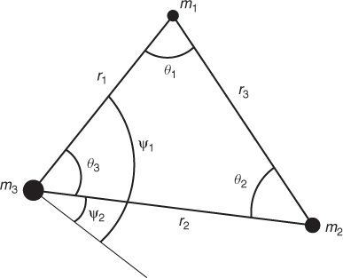
The rigidly rotating Lagrange triangle solution then has ψ2 = ωz, so that ψ1 = ωz + θ3, and constant values for the radii r1 and r2. The angles θ1, θ2, and θ3 are then determined from Equations 7.52, 7.53, 7.54, 7.55. At the steady state, Equations 7.53 and 7.55 for the angles ψ1 and ψ2 give
7.56 ![]()
On using the sine rule
7.57 ![]()
this becomes
By symmetry, we then have that the three-color Lagrange nematicon solution is
This gives the lengths of the sides of the triangle. Finally, the radial equations (Eqs 7.52 and 7.54) give the angular velocity of the rotating triangle as
In experimental situations the nonlocality parameter ν is large, ν = O(100) [20, 36]. Let us therefore examine the three-color Lagrange solution in the limit of ν ![]() 1. In this limit the potential (Eq. 7.47) can be approximated by
1. In this limit the potential (Eq. 7.47) can be approximated by
7.61 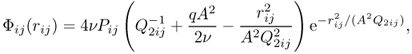
with
The first difference between the Lagrange solution for gravitation and for three-color nematicons is that the three-color potential (Eq. 7.61) is not monotonic as it is for Newtonian gravitation. Furthermore, the shape of the potential depends on the masses, whereas in the gravitation case the masses only scale the potential. It is then apparent that the three-color Lagrange solution will not be an equilateral triangle, as this uniform shape depends on the masses just scaling the potential. To see what possible shapes for the Lagrange three-color solution can occur, let us take advantage of the nonmonotonicity of the potential and construct a solution in the form of an elongated isosceles triangle. This particular solution is tractable using the large nonlocality limit (Eq. 7.61) of the potential. To this end, let us take two equal masses (optical powers) m2 = m3 and further assume that m2 ![]() m1. The triangle is then elongated with θ1 ∼ 0, θ2 = θ3 ≈ π/2 and r3 = r1 to leading order. From the general triangle solution (Eqs 7.59 and 7.60), we then obtain
m1. The triangle is then elongated with θ1 ∼ 0, θ2 = θ3 ≈ π/2 and r3 = r1 to leading order. From the general triangle solution (Eqs 7.59 and 7.60), we then obtain
The r3 in Equation 7.59 is then automatically satisfied by symmetry. Now because r2 is assumed to be the short side and r1 is assumed to be the long side of the triangle, we choose the large root of the first of Equation 7.63 and the small root of the second of Equation 7.63. We therefore see that an elongated isosceles triangle solution is possible for three nematicons. This solution is not possible for the monotone gravitational potential, but is natural for the nonmonotone nematicon potential.
Let us now study the linearized stability of the Lagrange three-color solution. Full details of this stability analysis can be found in Assanto et al. [29]. It is sufficient to note that the stability of the Lagrange three-color solution stems from the different slopes of the potential at the equilibrium positions of the nematicons. This again shows that the isosceles triangle shape is essential for stability when the potential is nonmonotone.
Unlike gravitating masses, nematicons are not rigid, but deform during their evolution and shed diffractive radiation. In Chapter 3 and in Section 7.3 it was shown how diffractive radiation generated from the shelf of low wave number radiation under an evolving nematicon provides a mechanism for mass loss, which in turn provides a damping that stabilizes nematicons. However, it is also known that the shedding of angular momentum in the form of a spiral wave can produce the collapse of a rotating coherent structure [37]. In light of this, let us now examine the effect of the spiral waves shed by the rotating three-color Lagrange structure.
To model the diffractive radiation shed by the jth-color nematicon, let us consider the linearized electric field equation (Eq. 7.39)
The linearized equation is appropriate as the radiation has small amplitude compared with the nematicon. In polar coordinates (ρ, φ) relative to the center of mass of the cluster, each nematicon moves in a circle of radius Rj with an angular position ζj(z). In effect, the nematicon acts as a source for the radiation equation (Eq. 7.64). Let us take the shelf under the jth nematicon to be of the form gj(ρ, φ − ζj(z)). The angular extent of the flat shelf is taken to be λj and the radial extent is taken as Rj − ϵ ≤ ρ ≤ Rj + ϵ. The detailed functional form of gj is not needed, but can be determined as detailed in Chapter 3 and in Section 7.3 using conservation of mass. We then need to solve the radiation equation (Eq. 7.64) together with the boundary condition
7.65 ![]()
Let us obtain the solution of the radiation equation (Eq. 7.64) using a geometric optics expansion. The validity of this geometric optics expansion is based on the relatively rapid rotation of the triangle. We therefore expand in the form
7.66 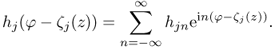
We then construct the solution for uj mode by mode in the geometric optics expansion form
7.67 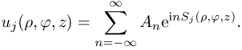
Substituting this geometric optics expansion into the radiation equation (Eq. 7.64) gives at first order the eikonal equation
7.68 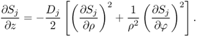
Higher order terms give transport equations for the An, but these will not be needed here. The boundary condition for the phase function S is
on using the boundary condition (Eq. 7.65). A separation of variables solution for S can hence be found as
This solution gives the phase of the spiral wave shed by the nematicon.
Substitution of the separation of variables solution (Eq. 7.70) into the eikonal equation (Eq. 7.68) gives the equation for Fj
with the boundary condition Fj(Rj + ϵ) = 0. It should be noted that as Fj = Fj(ρ) and ζj = ζj(z), this equation is inconsistent. The resolution of this is that the angular velocity ζj is a slowly varying function of z, and so can be taken as constant to the order considered here. We then have that the phase of the outgoing spiral wave is determined using the positive square root of Equation 7.71 as
7.72 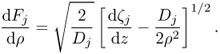
An asymptotic solution of this equation can be easily obtained for large ρ. Using this asymptotic form, the phase Sj of the spiral wave is
for large ρ, with the dot referring to derivatives with respect to z. It is clear from Equation 7.72 that for a spiral wave to exist the local rotation speed ![]() must satisfy
must satisfy
7.74 ![]()
If this relation is not satisfied the spiral waves are cut off. We then see that only rapidly rotating triangles shed spiral waves.
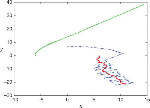
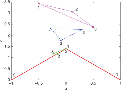
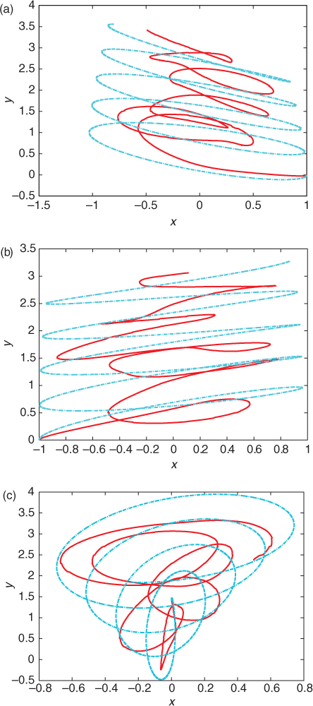
Figure 7.8 Position of nematicon peaks. z = 0 (solid line); z = 100 (cross); z = 200 (asterisk); z = 300 (square). 1 refers to u1, 2 refers to u2, and 3 refers to u3. Initial conditions are a1 = 1.8, w1 = 3.0, a2 = 1.8, w2 = 3.0, a3 = 1.44, w3 = 3.0, ξ1 = 1.0, η1 = 0.0, ξ2 = − 1.0, η2 = 0.0, ξ3 = 0.0, η3 = 1.4, U1 = 0.0, V1 = − 0.03, U2 = 0.0, V2 = 0.03, U3 = 0.038, and V3 = 0.0, with q = 10, ν = 500, D1 = 1.0, D2 = 0.95, D3 = 0.98, A1 = 1.0, A2 = 0.9, and A3 = 0.95. (Source: Reproduced with permission from Figure 7.1 in Reference 29.)
We shall now show how this cutoff behavior prevents the Lagrange cluster from collapsing. To do this, we shall calculate the loss of angular momentum from the jth nematicon and show that its angular momentum settles to an equilibrium value. The total angular momentum lj of the jth-color nematicon is
The loss of angular momentum at the edge of the shelf of radiation under the nematicon is [33, 34]
To evaluate the integral in this loss expression we need the geometric optics solution for the radiation uj evaluated at the edge of the shelf. The boundary condition (Eq. 7.65) gives An = hjn. Using this relation, the loss expression (Eq. 7.76) becomes
7.77 
As the mass of the nematicon is Equation 7.51,
on using the classical mechanics expression for angular momentum. We then have a closed equation for the angular momentum lj.
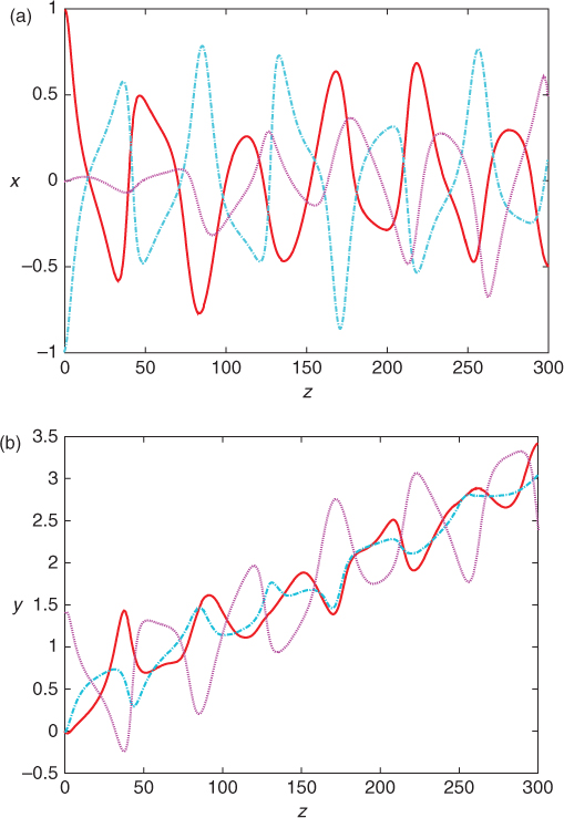
Figure 7.9 Numerical positions of three nematicons as a function of z: (a) x position and (b) y position. u1: solid line; u2: dot-dashed line; u3: dotted line. The initial conditions are a1 = 1.8, w1 = 3.0, a2 = 1.8, w2 = 3.0, a3 = 1.44, w3 = 3.0, ξ1 = 1.0, η1 = 0.0, ξ2 = − 1.0, η2 = 0.0, ξ3 = 0.0, η3 = 1.4, U1 = 0.0, V1 = − 0.03, U2 = 0.0, V2 = 0.03, U3 = 0.038, and V3 = 0.0, with q = 10, ν = 500, D1 = 1.0, D2 = 0.95, D3 = 0.98, A1 = 1.0, A2 = 0.9, and A3 = 0.95. (Source: Reproduced with permission from Figure 7.2 in Reference 29.)
Equation 7.77 shows that, initially, the nematicons slow due to the loss of angular momentum. As they slow, the spiral waves are eventually cut off owing to the cutoff condition (Eq. 7.74). After this point, the angular momentum of the coherent Lagrange triangle is conserved and the structure is stable.
The earlier analysis shows that isosceles triangle Lagrange solutions are stable and produce no diffractive radiation after they settle to the stable motion state. These theoretical predictions were tested by numerically solving the three-color nematicon equations (Eqs 7.39 and 7.40) with an equilateral triangle initial condition. Figure 7.8 shows a typical example, which has astronomical equivalents [38]. It can be seen that the structure undergoes dramatic reshaping as it rotates and translates, the translation being due to the initial linear momentum of the center of mass. It is further seen that the structure is reshaping itself into an isosceles triangle, confirming our stability analysis. More detailed views of the positions of the three nematicons in the Lagrange structure is shown in Figure 7.9. These detailed x and y positions confirm that the nematicons are orbiting about each other, with a general translation of the structure in the y direction.
A detailed comparison between the full numerical solution and the solution of the modulation equations is shown in Figure 7.10. The agreement between the numerical and modulation solutions is surprisingly good, given the drastic simplifications made to derive the modulation equations. The modulation solution reproduces the broad features of the motion, with the quantitative differences due to the reshaping of the nematicons, as discussed in Section 7.3. The assumptions used to derive the modulation equations (Eq. 7.50) were even more restrictive compared to those discussed in Section 7.3 as it was assumed that the amplitude and width of the nematicons were fixed.
Figure 7.10 Comparison of nematicon position between the numerical (solid line) and modulation solutions (dot-dashed line). Initial conditions are  , and V3 = 0.0, with q = 10, ν = 500, D1 = 1.0, D2 = 0.95, D3 = 0.98, A1 = 1.0, A2 = 0.9, and A3 = 0.95. (Source: Reproduced with permission from Figure 7.4 in Reference [29].)
These numerical and modulation results suggest that the rotating Lagrange isosceles triangle solution is strongly attractive. We therefore expect that three color clusters with angular momentum will reshape and radiate diffractive radiation, to eventually settle into an isosceles triangle configuration.
7.5 Vortex Cluster Interactions
Another analog with Newtonian gravitation, which could be of interest, is that of Saturn's rings interacting with the small moons, called shepherding moons, which occur in the vicinity of the rings, or even orbit within the rings. The nematicon analog of this gravitational interaction is a central vortex in one color interacting with nematicon beams. For simplicity, let us take a vortex interacting with two nematicon beams. There is the possibility of a strong distortion of the stable vortex due to a resonance between the angular motion of the dipole formed by the nematicons and the normal modes of the vortex. This is the same mechanism proposed by Maxwell [39] in his continuum theory of the rings of Saturn. This theory predicted that sustained tidal-like waves could be produced by the moons orbiting around the rings.
To test this Saturn-like configuration for the three-color nematicon equations (Eqs 7.39 and 7.40), these equations were numerically solved for the initial conditions
7.79 ![]()
with
7.80 ![]()
Here, (ρ, φ) are polar coordinates in the (x,y) plane.
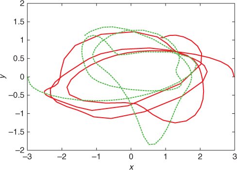
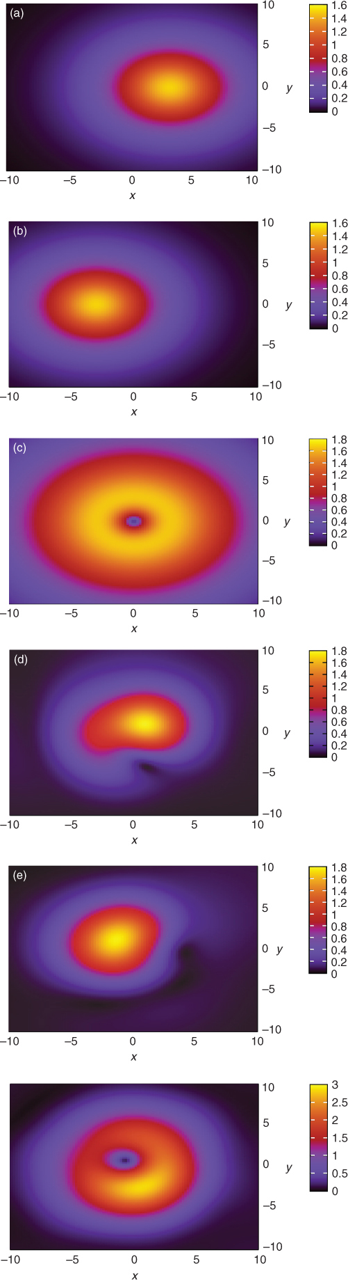
Figure 7.11 shows the trajectories of the two nematicons u1 and u2 up to z = 200. It can be seen that, whereas the individual trajectories are complicated, the two nematicons are orbiting about the origin, which is the position of the center of the vortex u3. The two nematicons u1 and u2 orbit at smaller radii than their initial values. The reason for this can be seen from the initial values at z = 0 and numerical solutions at z = 200 for u1, u2, and u3 shown in Figure 7.12. The vortex has evolved to have a smaller radius and the two nematicons have moved to be located on the ring on which the vortex has its maximum as this is the center of the waveguide induced by the vortex. The two nematicons have also distorted the symmetric shape of the vortex. Although the modulation equations governing nonlinear beams in liquid crystals are of the same form as those governing gravitating masses, nonlinear beams are not rigid masses and their distortion introduces dynamical effects that are not present in gravitation. To include the distortion of the vortex using modulation theory, we would need to include the evolution of its internal modes, as studied in Chapter 15, and obtain a wave-type equation for the evolution of its width forced by the motion of the nematicon beams. The comparison of the results of this extended modulation theory with Maxwell's theory for the waves generated in Saturn's rings would be an interesting extension of the theory of this chapter.
Figure 7.11 Positions of u1 color (solid line) and u2 color (dashed line) as given by full numerical solution (Eqs. 7.39 and 7.40) for initial conditions (Eq. 7.79). Parameter values are a10 = 1.5, w10 = 3.0, a20 = 1.5, w20 = 3.0, a30 = 1.5, w30 = 3.0, ξ10 = 3.0, η10 = 0.0, ξ20 = − 3.0, η20 = 0.0, U10 = 0.0, V10 = 0.05, U20 = 0.0, and V20 = − 0.05, with q = 10, ν = 500, D1 = 1.0, D2 = 0.95, D3 = 0.98, A1 = 1.0, A2 = 0.9, and A3 = 0.95.
Recently, other types of gravitational clusters with periodic structures have been investigated and their solution forms derived [40]. It would be of interest to study the nematicon equivalents of these gravitational clusters and determine the influence of the nonmonotonic nematicon potential (7.29) on their existence and stability.
7.6 Conclusions
The modulation theory developed in Chapter 3 has been used to investigate the interaction of two and more nematicons, solitary waves in a nematic liquid crystal. The amplitude and width evolution of the nematicons essentially decouples from their position and velocity evolution. On totally decoupling the amplitude and width evolution from the position and velocity evolution, the modulation equations describing the position and velocity evolution of the nematicons are the same as those governing the interaction of masses in Newtonian gravitation. However, the interaction potential is more complicated than the inverse separation potential of Newtonian gravitation. The nematicon potential gives two orbits for two interacting nematicons, the one with the larger radius being stable and the other being unstable. Under the modulation theory approximation, the evolution of interacting nematicons is then governed by the same basic principles as is the case with gravitating masses, these being conservation of total momentum and energy. The principal difference between the interaction of nematicons and gravitating masses is that interacting nematicons shed diffractive radiation in order to evolve to a steady state. Normally, gravitating bodies do not shed mass in order to reach stable orbits. Another difference between gravitating masses and interacting nematicons is that nematicons need a minimum mass, otherwise they break up into diffractive radiation. Furthermore, above a critical mass, they will break up into multiple nematicons. The close analogy between gravitating masses and interacting nematicons means that classical solutions from Newtonian gravitation can be carried over to the latter field, for instance, the Lagrange three-body solution discussed here.
Figure 7.12 Numerical solution of Equations 7.39 and 7.40 for initial conditions (Eq. 7.79). (a) |u1| at z = 0, (b) |u2| at z = 0, (c) |u3| at z = 0, (d) |u1| at z = 200, (e) |u2| at z = 200, (f) |u3| at z = 200. Parameter values are a10 = 1.5, w10 = 3.0, a20 = 1.5, w20 = 3.0, a30 = 1.5, w30 = 3.0, ξ10 = 3.0, η10 = 0.0, ξ20 = − 3.0, η20 = 0.0, U10 = 0.0, V10 = 0.05, U20 = 0.0, and V20 = − 0.05, with q = 10, ν = 500, D1 = 1.0, D2 = 0.95, D3 = 0.98, A1 = 1.0, A2 = 0.9, and A3 = 0.95. (Continued)
The analogy between interacting nematicons and gravitating masses can be pushed further. In addition to solitary wave beams (nematicons), the nematicon equations possess stable vortex solutions. Such vortices are analogous to many interacting masses, for example, the rings of Saturn and the other gas giants of the solar system or the asteroid belt. Nematicons can interact with such a vortex in a manner similar to the shepherding moons of Saturn. These analogies between interacting nematicons and gravitating masses can be further utilized to gain insight into and understanding of the interaction and evolution of nematicons.
Appendix: Integrals
The integrals Ii and Ii, j arising in the modulation equations are
7.A.1 
For a sech beam profile f(ζ) = sech ζ
7.A.2 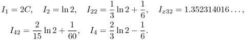
Here, C is the Catalan constant, C = 0.915965594 … [41]. For a Gaussian beam profile f(ζ) = exp( − ζ2)
7.A.3 ![]()
The constants A and B arising in the modulation equations are
7.A.4 ![]()
Acknowledgments
This research was supported by the Royal Society of London under Grant No. JP090179.
1. Y. S. Kivshar and G. Agrawal. Optical Solitons: From Fibers to Photonic Crystals. Academic Press, San Diego, CA, 2003.
2. G. Assanto, N. F. Smyth, and A. L. Worthy. Two colour, nonlocal vector solitary waves with angular momentum in nematic liquid crystals. Phys. Rev. A, 78:013832, 2008.
3. M. Peccianti, C. Conti, G. Assanto, A. De Luca, and C. Umeton. All-optical switching and logic gating with spatial solitons in liquid crystals. Appl. Phys. Lett., 81:3335–3337, 2002.
4. S. V. Serak, N. V. Tabiryan, M. Peccianti, and G. Assanto. Spatial soliton all-optical logic gates. IEEE Photon. Technol. Lett., 18:1287–1289, 2006.
5. A. Pasquazi, A. Alberucci, M. Peccianti, and G. Assanto. Signal processing by opto-optical interactions between self-localized and free propagating beams in liquid crystals. Appl. Phys. Lett., 87:261104, 2005.
6. G. Assanto and M. Peccianti. Routing light at will. J. Nonl. Opt. Phys. Mater., 16:37–48, 2007.
7. A. Alberucci, A. Piccardi, U. Bortolozzo, S. Residori, and G. Assanto. Nematicon all-optical control in liquid crystal light valves. Opt. Lett., 35:390–392, 2010.
8. M. Peccianti, K. A. Brzdakiewicz, and G. Assanto. Nonlocal spatial soliton interaction in nematic liquid crystals. Opt. Lett., 27:1460–1462, 2002.
9. A. Fratalocchi, A. Piccardi, M. Peccianti, and G. Assanto. Nonlinear management of the angular momentum of soliton clusters: Theory and experiments. Phys. Rev. A, 75:063835, 2007.
10. A. Fratalocchi, M. Peccianti, C. Conti, and G. Assanto. Spiraling and cyclic dynamics of nematicons. Mol. Cryst. Liq. Cryst., 421:197–207, 2004.
11. S. Lopez-Aguayo, A. S. Desyatnikov, Y. S. Kivshar, S. Skupin, W. Krolikowski, and O. Bang. Stable rotating dipole solitons in nonlocal optical media. Opt. Lett., 31:1100–1102, 2006.
12. D. Buccoliero, S. Lopez-Aguayo, S. Skupin, A. S. Desyatnikov, O. Bang, W. Krowlikowski, and Y. S. Kivshar. Spiraling solitons and multipole localized modes in nonlocal nonlinear media. Physica B, 394:351–356, 2007.
13. G. Assanto, M. Peccianti, K. A. Brzdkiewicz, A. De Luca, and C. Umeton. Nonlinear wave propagation and spatial solitons in nematic liquid crystals. J. Nonlin. Opt. Phys. Mater., 12:123–134, 2003.
14. J. F. Henninot, M. Debailleul, and M. Warenghem. Tunable non-locality of thermal non-linearity in dye doped nematic liquid crystal. Mol. Cryst. Liq. Cryst., 375:631–640, 2002.
15. J. F. Henninot, J. F. Blach, and M. Warenghem. Experimental study of the nonlocality of spatial optical solitons excited in nematic liquid crystal. J. Opt. A: Pure Appl. Opt., 9:20–25, 2007.
16. Y. V. Izdebskaya, V. G. Shvedov, A. S. Desyatnikov, W. Z. Krolikowski, M. Belic, G. Assanto, and Y. S. Kivshar. Counterpropagating nematicons in bias-free liquid crystals. Opt. Express, 18:3258–3263, 2010.
17. C. García-Reimbert, A. A. Minzoni, T. R. Marchant, N. F. Smyth, and A. L. Worthy. Dipole soliton formation in a nematic liquid crystal in the nonlocal limit. Physica D, 237:1088–1102, 2008.
18. B. D. Skuse and N. F. Smyth. Two-colour vector soliton interactions in nematic liquid crystals in the local response regime. Phys. Rev. A, 77:013817, 2008.
19. A. Alberucci, M. Peccianti, G. Assanto, A. Dyadyusha, and M. Kaczmarek. Two-color vector solitons in nonlocal media. Phys. Rev. Lett., 97:153903, 2006.
20. C. Conti, M. Peccianti, and G. Assanto. Route to nonlocality and observation of accessible solitons. Phys. Rev. Lett., 91:073901, 2003.
21. C. Conti, M. Peccianti, and G. Assanto. Observation of optical spatial solitons in a highly nonlocal medium. Phys. Rev. Lett., 92:113902, 2004.
22. C. García-Reimbert, A. A. Minzoni, N. F. Smyth, and A. L. Worthy. Large-amplitude nematicon propagation in a liquid crystal with local response. J. Opt. Soc. Am. B, 23:2551–2558, 2006.
23. G. Assanto, B. D. Skuse, and N. F. Smyth. Optical path control of spatial optical solitary waves in dye-doped nematic liquid crystals. Photon. Lett. Poland, 1:154–156, 2009.
24. G. Assanto, B. D. Skuse, and N. F. Smyth. Solitary wave propagation and steering through light-induced refractive potentials. Phys. Rev. A, 81:063811, 2010.
25. D. J. Kaup and A. C. Newell. Solitons as particles, oscillators, and in slowly changing media: a singular perturbation theory. Proc. R. Soc. London, Ser. A, 361:413–446, 1978.
26. I. M. Gelfand and S. V. Fomin. Calculus of Variations. Prentice-Hall, Englewood Cliffs, NJ, 1963.
27. H. Goldstein. Classical Mechanics. Addison-Wesley, Reading, MA, 1981.
28. G. Assanto, A. A. Minzoni, and N. F. Smyth. Light self-localization in nematic liquid crystals: modelling solitons in nonlocal reorientational media. J. Nonlin. Opt. Phys. Mater., 18:657–691, 2009.
29. G. Assanto, C. García-Reimbert, A. A. Minzoni, N. F. Smyth, and A. L. Worthy. Lagrange solution for three wavelength solitary wave clusters in nematic liquid crystals. Physica D, 240:1213–1219, 2011.
30. G. Assanto, A. A. Minzoni, M. Peccianti, and N. F. Smyth. Optical solitary waves escaping a wide trapping potential in nematic liquid crystals: modulation theory. Phys. Rev. A, 79:033837, 2009.
31. B. D. Skuse and N. F. Smyth. Interaction of two colour solitary waves in a liquid crystal in the nonlocal regime. Phys. Rev. A, 79:063806, 2009.
32. A. A. Minzoni, N. F. Smyth, and A. L. Worthy. Modulation solutions for nematicon propagation in non-local liquid crystals. J. Opt. Soc. Am. B, 24:1549–1556, 2007.
33. W. L. Kath and N. F. Smyth. Soliton evolution and radiation loss for the nonlinear Schrödinger equation. Phys. Rev. E, 51:1484–1492, 1995.
34. C. García-Reimbert, A. A. Minzoni, and N. F. Smyth. Spatial soliton evolution in nematic liquid crystals in the nonlinear local regime. J. Opt. Soc. Am. B, 23:294–301, 2006.
35. K. R. Simon. Mechanics, 2nd edn. Addison Wesley, Reading, 1960.
36. G. Assanto, M. Peccianti, and C. Conti. Optical spatial solitons in nematic liquid crystals: Nematicons. Opt. Phot. News, 14:45–48, 2003.
37. A. A. Minzoni, N. F. Smyth, and A. L. Worthy. Pulse evolution for a two dimensional Sine-Gordon equation. Physica D, 159:101–123, 2001.
38. J. A. Carter, D. C. Fabrycky, D. Ragozzine, M. J. Holman, S. N. Quinn, D. W. Latham, L. A. Buchhave, J. Van Cleve, W. D. Cochran, M. T. Cote, M. Endl, E. B. Ford, M. R. Haas, J. M. Jenkins, D. G. Koch, J. Li, J. J. Lissauer, P. J. MacQueen, C. K. Middour, J. A. Orosz, J. F. Rowe, J. H. Steffen, and W. F. Welsh. KOI-126: A triply eclipsing hierarchical triple with two low-mass stars. Science, 120 1274, 2011.
39. J. C. Maxwell. On theories of the constitution of Saturn's rings. Proc. R. Soc. Edinb., 4:99–101, 1862.
40. C. G. Azpetia. Aplicación del grado ortogonal en sistemas Hamiltonianos. Tesis Doctoral Universidad Nacional Autónoma de México, 2010.
41. M. Abramowitz and I. A. Stegun. Handbook of Mathematical Functions with Formulas, Graphs and Mathematical Tables. Dover Publications, New York, 1972.