
Chapter 1: Nematicons
1.1 Introduction
The term nematicon was coined to denote the material, nematic liquid crystals (NLC), supporting the existence of optical spatial solitons via a molecular response to light, a reorientational nonlinearity. Nematicons was first used in the title of Reference 1, after three years since the first publication on reorientational spatial optical solitons in NLC [2]. Since then, a large number of results, including experimental, theoretical, and numerical, have been presented in papers and conferences and formed a body of literature on the subject. In this chapter we attempt to summarize the most important among them, leaving the details to the specific articles but trying to provide a feeling of the amount of work carried out in slightly more than a decade.
1.1.1 Nematic Liquid Crystals
Liquid crystals are organic mesophases featuring various degrees of spatial order while retaining the basic properties of a fluid. In the absence of absorbing dopants, they are excellent dielectrics, transparent from the ultraviolet to the mid-infrared, with highly damaged thresholds, relatively low electronic susceptibilities, and significant birefringence at the molecular level and in the nematic phase. In the latter phase, their elongated molecules have the same average angular orientation, although their individual location is randomly distributed as they are free to move (Fig. 1.1a). NLC exhibit a molecular nonlinearity; when an electric field is present, the electrons in the molecular orbitals tend to oscillate with it and give rise to dipoles which, in turn, react to and tend to align with the field in order to minimize the resulting Coulombian torque [3–5] (Fig. 1.1b–c). This torque is counteracted by the elastic forces stemming from intermolecular links: equilibrium is established when the free energy of the system is minimized, as modeled by a set of Euler–Lagrange equations. Because the polarizability of the molecules is higher along their major axes, their reorientation toward the field will increase the optical density, both at the microscopic and macroscopic levels. It is noteworthy that an initial orthogonality between the field and the induced molecular dipoles corresponds to a threshold effect known as Freedericksz transition [3]. For static or low frequency fields, reorientation leads to a large electro-optic response with a positive refractive index variation for light polarized in the same plane of the field lines and the long molecular axes [3]. For fields at optical frequencies, the average angular orientation or molecular director in the nematic phase corresponds to the optic axis of the equivalent uniaxial crystal; hence, the refractive index for extraordinarily polarized electric fields (i.e., with field vector coplanar with both optic axis and wave-vector) will increase with the orientation angle θ (Fig. 1.1c–d for wave-vectors along z).
Figure 1.1 (a) Sketch of molecular distribution in the nematic phase and definition of director ![]() ; the ellipses represent NLC molecules. (b) Director orientation in the absence of electric field: the angle θ0 is determined by anchoring at the boundaries. (c) In a positive uniaxialNLC, a linearly polarized electric field can induce dipoles and rotate the molecular director towards its vector; the resulting stationary angle θ is determined by the equilibrium between the electric torque and the elastic intemolecular links. (d) Extraordinary refractive index versus angle between wave vector and director for a positive uniaxial NLC with n|| = 1.7 and n⊥ = 1.5.
; the ellipses represent NLC molecules. (b) Director orientation in the absence of electric field: the angle θ0 is determined by anchoring at the boundaries. (c) In a positive uniaxialNLC, a linearly polarized electric field can induce dipoles and rotate the molecular director towards its vector; the resulting stationary angle θ is determined by the equilibrium between the electric torque and the elastic intemolecular links. (d) Extraordinary refractive index versus angle between wave vector and director for a positive uniaxial NLC with n|| = 1.7 and n⊥ = 1.5.

The reorientational mechanism described above is neither instantaneous nor fast (see Chapter 13), but can be very large, with effective Kerr coefficients n2 of about 10−4 cm/W2 [6], that is, eight to twelve orders of magnitude larger than that in CS2 and in electronic media, respectively [7]. Therefore, nonlinear effects can be observed in NLC even with continuous wave lasers, at variance with many other nonlinear dielectrics often requiring pulsed excitations.
Nevertheless, the reorientational response is not the only available response in NLC. Owing to their fluidic nature, a high electric field can change the portion of molecules aligned to the director, that is, can affect the order parameter [8], particularly in the presence of dye dopants [9]. Doped NLC also features an enhanced reorientational nonlinearity because of the Janossy effect [10]. As a result of thermo-optic effect, a nonlinear response also stems from temperature changes, modifying the refractive indices mainly via the order parameter in phase transitions [6] (see Chapter 9). Moreover, NLC can show the photorefractive effect [4] and fast electronic nonlinearities (see Chapter 14).
1.1.2 Nonlinear Optics and Solitons
In nonlinear optics, the basic example of an intensity-dependent refractive index is the Kerr response n(I) = n0 + n2I. When n2 is positive, the index increases with the light intensity and, in the case of a finite beam, it gives rise to a lens-like refractive distribution, which is capable of self-focusing the excitation. Such a mechanism can actually compensate for the natural diffraction of the beam, resulting (in the simplest case) in a size/profile-invariant spatial soliton. Otherwise stated, the excitation beam deforms the refractive index distribution of the nonlinear (initially uniform) dielectric, generating a transverse graded-index profile that acts as a waveguide, that is, confines the field into a guided mode. The fundamental soliton in space is the lowest order mode guided by the self-induced dielectric waveguide. Spatial solitons of a Kerr nonlinearity, the so-called Townes solitons [11], tend to be unstable in two transverse dimensions because the exact balance of diffraction and self-focusing is achieved at a critical power [12, 13]. They are stable in one dimension (e.g., in planar waveguides [14]) or in the presence of higher order effects as compared to the Kerr law, such as saturation of the nonlinear change in index [15, 16], multiphoton absorption [17], discreteness [18, 19], and nonlocality [20]. In most cases they are observable in actual media although, being no longer exact solutions of an integrable differential system, they should be rigorously referred to as spatial solitary waves [21]. The terms soliton and solitary wave are interchangeably used throughout this chapter.
1.1.3 Initial Results on Light Self-Focusing in Liquid Crystals
As discussed in Section 1.1.1, several terms can contribute to the nonlinear response of NLC. Experiments conducted in the early 1980s demonstrated that, in undoped NLC, the dominant contribution is the reorientational nonlinearity [6, 22, 23]. An equivalent Kerr response was measured with light beams passing through the thickness of a planar cell, the latter behaving as a lens, the focus of which is dependent on the input power. For Rayleigh distances much smaller than the NLC layer thickness, rings could be observed in the diffraction pattern [24].
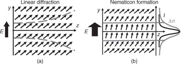
An experiment on self-focusing in the bulk of a dye-doped NLC layer was carried out in 1993 by Braun et al. [25], who imaged the scattered light from a beam propagating in a cylindrical geometry with NLC subject to Freedericksz threshold. Various phenomena were observed, including undulation, filamentation, and nonstationary evolution along the capillary; they were interpreted and modeled with joint reorientational and nonlinear Schrödinger equations [26, 27]. After such a pioneering work, self-localization of light as a consequence of thermo-optic effects in capillaries was reported by Derrien et al. [28]; the interplay between thermal and reorientational responses was addressed by Warenghem et al. [29] (see Chapter 9). The use of suitably built planar cells with the director tilted by an external bias to avoid the Freedericksz threshold allowed Peccianti et al. to observe the profile-invariant spatial solitons at a few milliWatts [2]. Unbiased planar cells with pretilt determined by rubbing permitted the detailed study of walk-off [30] (see Chapter 6). Figure 1.2 sketches the basic mechanism of nematicon formation via a purely reorientational response.
Figure 1.2 Basic physics of nematicons. An extraordinarily polarized bell-shaped beam with wave-vector along ![]() is launched in an NLC layer with director lying in the plane yz. The major axes of the molecules are at an angle
is launched in an NLC layer with director lying in the plane yz. The major axes of the molecules are at an angle ![]() with the wave-vector, thanks to a pretilt (the arrows indicate the molecular director). (a) In the linear regime light does not affect the angular distribution of the director: the beam diffracts as in homogeneous media. (b) Conversely, at high powers the director is perturbed and reorientates toward
with the wave-vector, thanks to a pretilt (the arrows indicate the molecular director). (a) In the linear regime light does not affect the angular distribution of the director: the beam diffracts as in homogeneous media. (b) Conversely, at high powers the director is perturbed and reorientates toward ![]() , increasing θ and thus the refractive index (Fig. 1.1d). The perturbation is stronger where the intensity I is higher; hence, an index well is created by the light beam itself, leading to the formation of a waveguide and a self-trapped nematicon. Noticeably, the perturbation extends far beyond the beam profile owing to the elastic links between molecules. For the sake of simplicity, in this illustration the role of walk-off is ignored (Section 1.2.1).
, increasing θ and thus the refractive index (Fig. 1.1d). The perturbation is stronger where the intensity I is higher; hence, an index well is created by the light beam itself, leading to the formation of a waveguide and a self-trapped nematicon. Noticeably, the perturbation extends far beyond the beam profile owing to the elastic links between molecules. For the sake of simplicity, in this illustration the role of walk-off is ignored (Section 1.2.1).
Finally, nematicons were also reported in slab waveguides with homeotropically aligned NLC [31], in one-dimensional arrays of coupled waveguides [18, 32] (see Chapter 10) and in twisted/chiral NLC [33, 34] (see Chapter 12).
1.2 Models
In this section, we review the main theoretical results concerning nonlinear light propagation in NLC cells, with specific reference to a reorientational response supporting optical spatial solitons as well as modulational instability. We first discuss scalar geometries (voltage-biased cells), that is, those in which the role of birefringent walk-off can be left aside. Afterward, we consider the most general case of cells where the walk-off has a substantial effect.
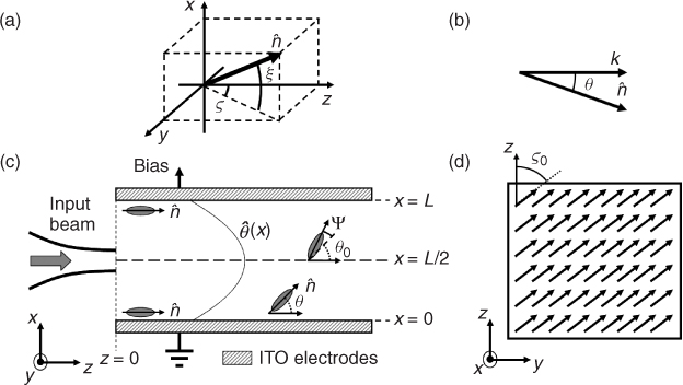
The director distribution can be described by the two polar angles ξ (tilt from the plane yz) and ζ (in the plane yz) (Fig. 1.3a). In addition, θ is the angle between the beam wave-vector ![]() and the molecular director
and the molecular director ![]() (Fig. 1.3b). In scalar geometries ζ = 0, the latter implying θ = ξ (Fig. 1.3c). In general, ζ ≠ 0 owing to the anchoring at the (glass/NLC) interfaces parallel to the plane yz; at rest the director
(Fig. 1.3b). In scalar geometries ζ = 0, the latter implying θ = ξ (Fig. 1.3c). In general, ζ ≠ 0 owing to the anchoring at the (glass/NLC) interfaces parallel to the plane yz; at rest the director ![]() lies in the plane yz at an angle ζ0 with z (Fig. 1.4d).
lies in the plane yz at an angle ζ0 with z (Fig. 1.4d).
Figure 1.3 (a) Definition of polar angles describing the director in the xyz space. (b) Definition of the angle θ between the wave-vector ![]() and the director
and the director ![]() . (c) Side view sketch of a biased planar NLC cell with anchoring condition at the interfaces such that
. (c) Side view sketch of a biased planar NLC cell with anchoring condition at the interfaces such that ![]() (i.e., θ = ξ) and a focused light beam launched along z. The structure is assumed to be infinitely extended along y. (d) Top view of a planar cell showing the rubbing angle ζ0 in the plane yz; the arrows represent the director distribution in the absence of external excitations (neither bias nor illumination).
(i.e., θ = ξ) and a focused light beam launched along z. The structure is assumed to be infinitely extended along y. (d) Top view of a planar cell showing the rubbing angle ζ0 in the plane yz; the arrows represent the director distribution in the absence of external excitations (neither bias nor illumination).
We stress that the equations and the results shown hereby hold valid in the limit of small optical perturbations; the highly nonlinear case is dealt with in Chapter 11.
1.2.1 Scalar Perturbative Model
We consider the configuration of Fig. 1.3c: a finite light beam is launched in the planar NLC cell with wave-vector along the z axis and the field linearly polarized along the x axis. Two parallel glass plates contain the NLC, with molecular director ![]() lying in the plane xz (i.e.,
lying in the plane xz (i.e., ![]() ) at an angle θ with
) at an angle θ with ![]() (i.e.,
(i.e., ![]() ). A low frequency electric field ELF is applied (via transparent electrodes on the plates) across
). A low frequency electric field ELF is applied (via transparent electrodes on the plates) across ![]() to overcome the Fréedericksz threshold and pretilt the molecules in the plane xz via the electro-optic response, creating a potential
to overcome the Fréedericksz threshold and pretilt the molecules in the plane xz via the electro-optic response, creating a potential ![]() in the absence of illumination;
in the absence of illumination; ![]() depends only on x due to the symmetry of the problem.
depends only on x due to the symmetry of the problem.
In this configuration the beam excites only the extraordinary component, generally at the walk-off δ with respect to ![]() , owing to birefringence. Hereby, we scalarize the problem and assume the electric field Eopt of the beam to be linearly polarized along
, owing to birefringence. Hereby, we scalarize the problem and assume the electric field Eopt of the beam to be linearly polarized along ![]() , leaving the vectorial case to Section 1.2.2. The use of a scalar model also implies neglecting the tilt between Poynting and wave-vectors. Let us define A, the slowly varying envelope of Eopt, that is,
, leaving the vectorial case to Section 1.2.2. The use of a scalar model also implies neglecting the tilt between Poynting and wave-vectors. Let us define A, the slowly varying envelope of Eopt, that is,
![]()
with θ0 the orientation without light and ![]() the extraordinary wave refractive index, where
the extraordinary wave refractive index, where ![]() (ϵ||) is the electronic susceptibility perpendicular (along) to
(ϵ||) is the electronic susceptibility perpendicular (along) to ![]() . In the paraxial approximation, light propagation is ruled by [2]
. In the paraxial approximation, light propagation is ruled by [2]
where k = k0ne(θ0) and we set θ = θ0 + Ψ, with Ψ being the light-induced perturbation on θ.
As we are interested in the reorientational nonlinearity, we need a further equation describing how the angle θ varies under the application of both Eopt and ELF. To this extent, minimization of the NLC free energy that assumes a single constant to describe the elastic (intermolecular) forces, yields the Euler–Lagrange equation [3, 35]
with ΔϵLF being the anisotropy and K the Frank elastic constant, and ![]() being
being ![]() [35]. Equation 1.2 is obtained when
[35]. Equation 1.2 is obtained when ![]() , that is, in the perturbative limit.
, that is, in the perturbative limit.
For straight beam trajectories (i.e., homogeneous medium, uniform director distribution, no walk-off) we can set ![]() . When
. When ![]() and the beam axis is in the cell mid-plane x = 0 with
and the beam axis is in the cell mid-plane x = 0 with ![]() , the light-induced reorientation is governed by [35]
, the light-induced reorientation is governed by [35]
that is, by a Yukawa (or screened Poisson) equation, with forcing term given by the light intensity and screening length l equal to
where we set ![]() and
and ![]() . It is straightforward to obtain
. It is straightforward to obtain ![]() and
and ![]() ; between these two extrema cl decreases monotonically. We note that θ0 depends only on the applied voltage V ≈ ELFL; hence, Equation 1.4 provides
; between these two extrema cl decreases monotonically. We note that θ0 depends only on the applied voltage V ≈ ELFL; hence, Equation 1.4 provides ![]() and for a given bias V, the spatial width of the nonlinear response is proportional to the cell thickness L.
and for a given bias V, the spatial width of the nonlinear response is proportional to the cell thickness L.
The system formed by Equations 1.1 and 1.3 governs nonlinear light propagation in biased NLC cells; for any NLC and cell size (i.e., thickness L), the parameters depend on the bias via the applied electric field and θ0, that is, on low frequency reorientation bias, including pretilt. Such a feature allows for electrically tuning both nonlinearity and nonlocality of the medium [36].
To quantify the nonlinearity, let us define the material-dependent parameter γ = ϵ0ϵa/(4K); using Equation 1.3, Ψ can be expressed via the Green formalism as
where ![]() is the Green function of the Yukawa equation (Eq. 1.3).
is the Green function of the Yukawa equation (Eq. 1.3).
Using Equation 1.5 the photonic potential [defined as ![]() and corresponding to the potential with a change in sign] reads
and corresponding to the potential with a change in sign] reads ![]()
![]() . We can thus write the effective (nonlocal) Kerr coefficient as
. We can thus write the effective (nonlocal) Kerr coefficient as
1.6 ![]()
The square dependence on the screening length l2 stems from the integral in Equation 1.5: for intensity distributions maintaining their transverse size with respect to l (i.e., ![]() invariant), the perturbation Ψ scales with l2. Conversely, the magnitude of the nonlocality, that is, the ratio between the widths of the photonic potential and the intensity profile, is determined by l. In fact, in the limit l → ∞, Equation 1.3 becomes a Poisson equation, with degree of nonlocality fixed by the boundaries (see Chapter 11 and references therein). After setting |A|2 = |B|2/l2, for l → 0 we get Ψ∝|B|2: in this regime NLC resemble local Kerr media.
invariant), the perturbation Ψ scales with l2. Conversely, the magnitude of the nonlocality, that is, the ratio between the widths of the photonic potential and the intensity profile, is determined by l. In fact, in the limit l → ∞, Equation 1.3 becomes a Poisson equation, with degree of nonlocality fixed by the boundaries (see Chapter 11 and references therein). After setting |A|2 = |B|2/l2, for l → 0 we get Ψ∝|B|2: in this regime NLC resemble local Kerr media.
1.2.1.1 Solitary Waves
Let us define the normalized coordinates ![]() ,
, ![]() , and Z = z; we also introduce the normalized quantities
, and Z = z; we also introduce the normalized quantities ![]() sin(2θ0)/(2K)Ψ and
sin(2θ0)/(2K)Ψ and ![]() , with α = 1/(2kl2). The parameter α is inversely proportional to nonlocality, that is, α is equal to zero if the nonlocality range is infinite, whereas it tends to ∞ in the local (Kerr) case. Equations 1.1 and 1.3 now read [35]
, with α = 1/(2kl2). The parameter α is inversely proportional to nonlocality, that is, α is equal to zero if the nonlocality range is infinite, whereas it tends to ∞ in the local (Kerr) case. Equations 1.1 and 1.3 now read [35]
Suppose ∂2ψ/∂Z2 = 0. From Equation 1.7 we can write ![]() . For large α we can write
. For large α we can write ![]() ; hence, light propagation is governed by the single equation [35]
; hence, light propagation is governed by the single equation [35]
Equation 1.9 describes nonlinear light propagation in a weakly nonlocal medium; it was shown in References 20, 35, and 37 how nonlocality inhibits catastrophic beam collapse. Conversely, if terms proportional to α−2 are neglected, Equation 1.9 transforms into a local NLSE (NonLinear Schrödinger Equation): solitary waves in (2+1)D are Townes-like and undergo catastrophic collapse [13]. Therefore, spanning the free parameter from zero to infinity, solitary waves evolve from accessible solitons (α = 0) [38] to Townes solitons [11] (α → ∞).
To confirm this qualitative assessment, let us look for soliton-like solutions of Equations 1.7 and 1.8 after setting ∂ψ/∂Z = 0 and a = v(X, Y)exp(iβZ). We obtain
with ψv the optical perturbation in presence of solitary waves. Interestingly, the system of Equations 1.10 and 1.11 determines the profile of solitary waves in parametric crystals as well [35, 39]. If the boundaries are circularly symmetric or if their influence can be neglected (see Chapter 11), the lowest order (i.e., single hump) solitary wave solutions of system (1.10) and (1.11) are radially symmetric. Thus, without loss of generality, we can expand ψv in a MacLaurin series around ![]() , that is, we write ψv = ψ0 + ψ2R2 + ψ4R4 +
, that is, we write ψv = ψ0 + ψ2R2 + ψ4R4 + ![]() , where the odd terms in R are zero due to the symmetry in the problem. In the highly nonlocal case [38, 40], the soliton waist is small compared to the size of the self-induced index well; hence, it is possible to set ψv ≈ ψ0 + ψ2R2. After substitution into Equation 1.11, the latter becomes the well-known model of the quantum harmonic oscillator, with oscillator strength depending on the beam power via Equation 1.10 [38, 40].
, where the odd terms in R are zero due to the symmetry in the problem. In the highly nonlocal case [38, 40], the soliton waist is small compared to the size of the self-induced index well; hence, it is possible to set ψv ≈ ψ0 + ψ2R2. After substitution into Equation 1.11, the latter becomes the well-known model of the quantum harmonic oscillator, with oscillator strength depending on the beam power via Equation 1.10 [38, 40].
Let us set f = |v|2 and, in analogy with what had been done above for ψv, expand f into f = f0 + f2R2 + f4R4 + ![]() ; Equation 1.10 then gives
; Equation 1.10 then gives
1.13 ![]()
having retained terms up to R2. In the highly nonlocal limit the soliton profile is Gaussian, that is, ![]() , where
, where ![]() is the normalized power; hence, it is straightforward to get
is the normalized power; hence, it is straightforward to get ![]() . At the same time, from quantum mechanics
. At the same time, from quantum mechanics ![]() . In the simplest case α = 0, Equation 1.12 provides
. In the simplest case α = 0, Equation 1.12 provides ![]() , yielding the condition for nematicon existence [40]:
, yielding the condition for nematicon existence [40]:
1.14 ![]()
1.2.1.2 Modulational Instability
In Section 1.2.1.1, we focused on bell-shaped wavepackets undergoing self-confinement through a reorientational response, underlining the stabilizing effect of nonlocality. In self-focusing media, spatial solitons are states of minimum energy; hence, lightwaves will evolve to these configurations whenever possible. An example of this is modulational instability: a plane wave in a self-focusing material is unstable and evolves first into a periodically modulated wavefront before it eventually forms multiple solitons. The spatial frequency components generated (i.e., amplified from noise at the expense of the zero frequency component) during propagation are dependent on the input power, with a spectral gain G(ky).
To model such processes, we can refer to Equations 1.7 and 1.8 in the one-dimensional limit (i.e., we set ∂/∂x = 0); we consider the plane wave solution ![]() to be consistent with the discussion in Section 1.2.1 (the power density is
to be consistent with the discussion in Section 1.2.1 (the power density is ![]() ) with ψPW = |a0|2 and βPW = |a0|2, and introduce a small perturbation by a = (aPW + Δa)exp(iβPWz) and ψ = ψPW + Δψ for amplitude and reorientation, respectively. For ∠a0 = 0, at the first order the gain coefficient G(ky) (i.e., the perturbation evolves as ∝exp[G(ky)z]) reads [41]
) with ψPW = |a0|2 and βPW = |a0|2, and introduce a small perturbation by a = (aPW + Δa)exp(iβPWz) and ψ = ψPW + Δψ for amplitude and reorientation, respectively. For ∠a0 = 0, at the first order the gain coefficient G(ky) (i.e., the perturbation evolves as ∝exp[G(ky)z]) reads [41]
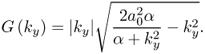
As anticipated, the modulational instability gain is dependent on the transverse frequency ky, with amplification changing with the input power density ![]() . In the limit α → ∞ Equation 1.15 yields
. In the limit α → ∞ Equation 1.15 yields ![]() , retrieving the correct expression for local Kerr media.
, retrieving the correct expression for local Kerr media.
1.2.2 Anisotropic Perturbative Model
In a generic (nonmagnetic) optically uniaxial medium, the electric field obeys [42]
where ![]() [4, 5], are the dielectric tensor components, δij is the Kronecker function, nj is the jth component of the director
[4, 5], are the dielectric tensor components, δij is the Kronecker function, nj is the jth component of the director ![]() ,
, ![]() is the anisotropy.
is the anisotropy.
Let us consider the extraordinary solution with wave-vector along z and write ![]() ; if A is a constant, the solution is a plane wave satisfying the tensorial equation [42]
; if A is a constant, the solution is a plane wave satisfying the tensorial equation [42]
1.17 ![]()
where the last equivalence stems from Equation 1.16 and I is the identity matrix. The effect of optical reorientation is to perturb the dielectric tensor so that ![]() , where
, where ![]() is the unperturbed tensor in the absence of light, and
is the unperturbed tensor in the absence of light, and ![]() is the light-induced perturbation; η plays the role of a small parameter, to be set to unity at the end of the derivation. We assume that the optic axis is at an angle θ with respect to the z axis (Fig. 1.3c). We use for convenience a new reference system xts obtained by rotating the original xyz around x by the walk-off angle δ; therefore, we get
is the light-induced perturbation; η plays the role of a small parameter, to be set to unity at the end of the derivation. We assume that the optic axis is at an angle θ with respect to the z axis (Fig. 1.3c). We use for convenience a new reference system xts obtained by rotating the original xyz around x by the walk-off angle δ; therefore, we get ![]() and
and ![]() .
.
After defining the slow scales r = r0 + ηr1 + ![]() + ηnrn with
+ ηnrn with ![]() , the electric field in xts can be expanded as
, the electric field in xts can be expanded as ![]()
![]() ; finally, the differential operator can be cast as ∇ = ∇0 + η∇1 +
; finally, the differential operator can be cast as ∇ = ∇0 + η∇1 + ![]() + ηn∇n. Imposing the solvability conditions (up to order η2) for Eopt and letting η → 1, we get [42]
+ ηn∇n. Imposing the solvability conditions (up to order η2) for Eopt and letting η → 1, we get [42]
where ![]() ,
, ![]() , and
, and ![]() are the diffraction coefficients, differing from unity because of anisotropy.
are the diffraction coefficients, differing from unity because of anisotropy.
If the mixed derivative can be neglected (small walk-off δ), Equation 1.18 is an NLSE modeling light propagation in the walk-off reference system. Equation 1.18 is valid in the perturbative regime, that is, when nonlinear variations on the dielectric tensor are small compared with its linear value; in this limit, photons propagate along the Poynting vector of the carrier plane wave, that is, walk-off does not depend on power. Furthermore, under these approximations the beam remains linearly polarized (other components appear at the next order, i.e., when Fe is accounted for) and paraxial with respect to s [43].
Equation 1.18 has to be solved with the reorientational equation for the nonlinear changes in director profile, allowing in turn to compute the photonic potential ![]() . For the configuration in Figure 1.3, the simplest case is when the cell is unbiased, with ξ = 0, θ = ζ, and consequently θ0 = ζ0; in fact, molecular rotation takes place only in yz, with θ governed by [44]
. For the configuration in Figure 1.3, the simplest case is when the cell is unbiased, with ξ = 0, θ = ζ, and consequently θ0 = ζ0; in fact, molecular rotation takes place only in yz, with θ governed by [44]
The photonic potential is
taking into account the smallness of Ψ. Vph has the same expression calculated in Section 1.2.1 in the limit δ → 0. By using elementary trigonometry, we can eliminate δ from Equation 1.20 and get [42]
1.21 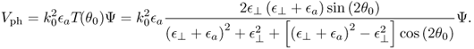
For ζ0 = 0 and applied bias, the configuration corresponds to the one in Section 1.2.1 with director moving in the plane xz; thus, Equation 1.3 is valid if the walk-off δ is included in the term modeling the torque; hence, all results derived in that section remain valid, specifically Equation 1.3 (with the torque correction just pointed out), which, jointly with Equations 1.18 and 1.20, is a complete model for vectorial nematicons propagating in the perturbative regime when the director reorients in the single plane xz.
When a bias is applied to the cell in Figure 1.3 with ζ0 ≠ 0, the reorientation dynamics becomes more complicated, as light and voltage induced torques tend to move the molecules in two different planes and two angles are needed to describe the director distribution (Fig. 1.3a) [3]. Owing to the symmetry, bias acts only on angle ξ, inducing in the absence of light a director profile equal to the case ζ0 = 0, that is, ![]() . To first approximation, the result is to modulate the magnitude of the screening term depending on the low frequency field, with an expected dependence on
. To first approximation, the result is to modulate the magnitude of the screening term depending on the low frequency field, with an expected dependence on ![]() [42]: in fact, at zero bias (
[42]: in fact, at zero bias (![]() ) the screening term is absent (see Section 1.2.2.1), whereas for
) the screening term is absent (see Section 1.2.2.1), whereas for ![]() we retrieve the case of Section 1.2.1.
we retrieve the case of Section 1.2.1.
1.2.2.1 Nematicon Breathers
In an unbiased cell with ζ0 ≠ 0, for small Ψ Equation 1.19 becomes
where δ0 = δ(θ0). Assuming a parabolic index well of the form ![]() , from Equation 1.22 the coefficient Ψ2 is [40]
, from Equation 1.22 the coefficient Ψ2 is [40]
where f0 = |A(x = L/2, t = 0)|2. We remark that the Equation 1.23 is obtained from Eq. 1.22 with no approximation, and thus is valid whenever the intensity profile and the nonlinear perturbation are radially symmetric.
The photonic potential becomes
1.24 ![]()
In analogy with quantum mechanics, the term proportional to Ψ0 is a rest energy, depending on the beam shape and boundary conditions and generally varying with s, that is, an equivalent time; in optics, it is responsible for nonlinear changes in the propagation constant. Conversely, the term Ψ2 determines the resonance frequency of the equivalent harmonic oscillator. Taking—for the sake of simplicity—Dx = Dt = D, from quantum harmonic oscillator theory we infer that the lowest order solitary wave of power Ps has the shape [38]
1.25 ![]()
where ![]() and
and ![]() are the nonlinear correction of propagation constant β due to the equivalent rest energy (increase in β) and the parabolic potential (decrease in β), respectively. The soliton width ws and power Ps are not independent variables owing to the dependence of Ψ2 on power; we find [38, 40, 42]
are the nonlinear correction of propagation constant β due to the equivalent rest energy (increase in β) and the parabolic potential (decrease in β), respectively. The soliton width ws and power Ps are not independent variables owing to the dependence of Ψ2 on power; we find [38, 40, 42]
For small Ψ0, Equation 1.26 reduces to ![]() ; thus, the nematicon properties do not depend on the boundary conditions. Equation 1.26 is the existence curve for single-hump nematicons in unbiased cells and in the highly nonlocal approximation.
; thus, the nematicon properties do not depend on the boundary conditions. Equation 1.26 is the existence curve for single-hump nematicons in unbiased cells and in the highly nonlocal approximation.
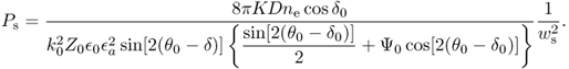
The next step is to investigate light propagation for a Gaussian beam launched in the NLC cell, but with waist w and power P not satisfying Equation 1.26. Assuming a parabolic approximation for the index distribution, we can still refer to the harmonic oscillator to model self-confinement. Using a generalization of the Ehrenfest theorem, the waist w is governed by [45]
where ![]() with F(θ0) = sin[2(θ0 − δ0)] + Ψ0cos[2(θ0 − δ0)]. If w changes only slightly in propagation (w − ws
with F(θ0) = sin[2(θ0 − δ0)] + Ψ0cos[2(θ0 − δ0)]. If w changes only slightly in propagation (w − ws ![]() ws) and ws is large enough to neglect the terms depending on
ws) and ws is large enough to neglect the terms depending on ![]() with respect to those proportional to
with respect to those proportional to ![]() , Equation 1.27 can be recast as [40]
, Equation 1.27 can be recast as [40]
Equation 1.28 can be analytically solved, yielding [40]
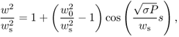
with w0 being the initial waist and ws = ws(P) the soliton waist corresponding to an input power P through Equation 1.26. We assumed a flat phasefront at the input. Equation 1.29 predicts a sinusoidal oscillation of the waist along propagation, that is, breathing self-confined wavepackets [38, 40, 42]. In particular, if w0 > ws, the nonlinearity dominates on diffraction at the input, the beam initially focuses; if w0 < ws, the roles are inverted and the beam initially expands. The oscillation amplitude is proportional to the distance from the solitary wave condition (i.e., |w0 − ws|), and the oscillation period Λ is ![]() . From Equations 1.29 and 1.26, the breathing periodicity is inversely related to the input power P (Λ∝P−1), that is, larger powers correspond to faster changes in the nematicon waist.
. From Equations 1.29 and 1.26, the breathing periodicity is inversely related to the input power P (Λ∝P−1), that is, larger powers correspond to faster changes in the nematicon waist.
We stress that all results derived in this section for unbiased cells apply as well to biased cells with ζ0 = 0, with straightforward corresponding expressions, once the strength of the nonlinear harmonic oscillator is calculated from Equation 1.23.
1.3 Numerical Simulations
1.3.1 Nematicon Profile
The profile of paraxial nematicons in unbiased cells can be evaluated numerically from Equations 1.18 and 1.19 by setting ∂sΨ = 0, θ = θu(x, t), and ![]() , where Z0 is the vacuum impedance, P the soliton power, and β the nonlinear correction to the propagation constant. We obtain the nonlinear eigenvalue problem
, where Z0 is the vacuum impedance, P the soliton power, and β the nonlinear correction to the propagation constant. We obtain the nonlinear eigenvalue problem
The system of Equations 1.30 and 1.31 can be solved using a standard relaxation scheme. We consider the NLC mixture E7, often employed in experiments. Its refractive indices versus wavelength are plotted in Figure 1.4, and the Frank elastic constant is 12 × 10−12N.
Figure 1.4 Refractive index versus wavelength in the NLC mixture E7, for electric field parallel (top line) and perpendicular (bottom line) to the director (optic axis). Symbols are data and solid lines represent the interpolations using a dispersion model.
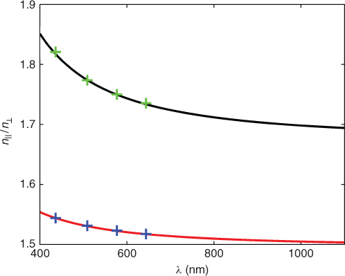
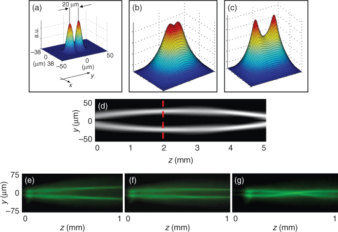
Figure 1.5a–d shows the numerically computed results for a single-hump soliton at P = 1 mW. Even if the diffraction coefficients Dx and Dt are unequal, the intensity profile is radially symmetric to a very good approximation. Moreover, if the nematicon waist is small with respect to the cell thickness L, the shape of θu is nearly symmetric around the beam, despite the boundary conditions with strong anchoring at the glass interfaces. Figure 1.5e and f plots light and director along s computed with a BPM (Beam Propagation Method) code for P = 1 mW nematicon profile at the input: both θ and u are invariant in propagation.
Figure 1.5 (a) Electric field profile u and (b) director distribution θu in the plane xt for a nematicon of power 1 mW. Graphs of (c) u and (d) θu in plane x = L/2 (gray line) versus t and in plane t = 0 versus x (black line). Computed 3D (e) intensity profile and (f) director distribution for an input beam as in (a). The wavelength is 632.8 nm, θ0 = π/6, and the cell thickness L is 100 μm.
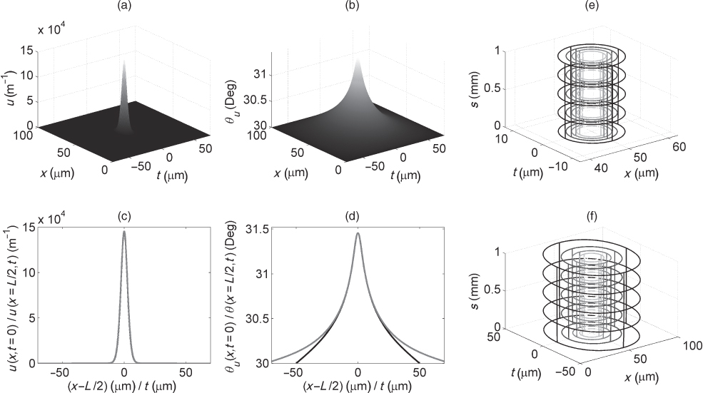
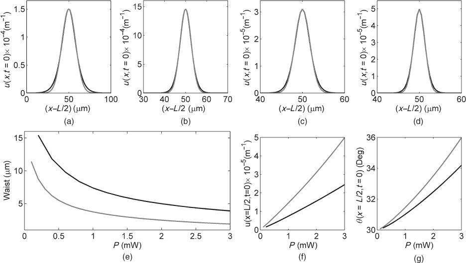
Figure 1.6 displays nematicon profiles for various input powers. The transverse intensity distribution is quite close to Gaussian, with small departures in the tails (Figure 1.6a–d). The nematicon existence curve versus power and waist is approximately given by P∝w−2, consistently with the model of accessible solitons (Fig. 1.6e). For a given power, the nematicon is narrower at shorter wavelengths due to reduced diffraction, as predictable; such a stronger confinement is also demonstrated by higher intensity peaks and larger maxima in director orientation, as in Figure 1.6f and g, respectively.
Figure 1.6 Nematicon profile for (a) P = 0.1, (b) 1, (c) 2, and (d) 3 mW versus x − L/2 at λ = 632.8 nm; dark and gray lines are exact numerical results and Gaussian best-fit, respectively. (e) Waist, (f) peak of the electric field u, and (g) maximum of θu for solitary waves versus power P at λ = 632.8 nm (gray line) and λ = 1064 nm (black line). Here, θ0 = π/6 and L = 100 μm.
1.3.2 Gaussian Input
For a direct comparison with experimental data, it is important to investigate light evolution in the case of a Gaussian beam injected into the NLC layer.
We take an input excitation
1.32 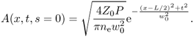
of power P and waist w0. We numerically solve the system [46]
1.33 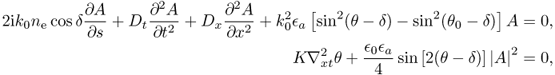
where we neglected longitudinal derivatives in the reorientational equation. Figure 1.7 plots the evolution of a red beam (λ = 632.8 nm) for θ0 = π/6, P = 1 mW, and w0 = 3.5 μm; we define ![]() and It(t, s) =
and It(t, s) = ![]() , the transverse integrals of the intensity. In experiments, Ix and It are proportional to the scattered light acquired by a camera to monitor the beam evolution in the sample.
, the transverse integrals of the intensity. In experiments, Ix and It are proportional to the scattered light acquired by a camera to monitor the beam evolution in the sample.
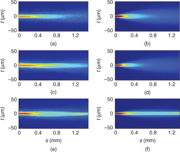
Figure 1.7 Beam evolution for P = 1 mW, w0 = 3.5 μm, and λ = 632.8 nm. (a and b) Ix in the plane xs. (c and d) It in the plane ts. 3D profiles of (e) intensity |A|2 and (f) director perturbation. Here, L = 100 μm and θ0 = π/6.
Because the initial conditions do not correspond to a point in the existence curve, a breather gets excited, with a quasi-sinusoidal oscillation in the waist along s; by the entrance (i.e., near s = 0) the beam narrows as in the plane waist-power the input profile lies above the existence curve: self-focusing prevails on diffractive spreading. We also note that the self-confined wave retains its radial symmetry, consistently with the results of Section 1.3.1. Finally, even if the waist oscillates with s, the distribution of θ remains nearly constant (Fig. 1.7f).
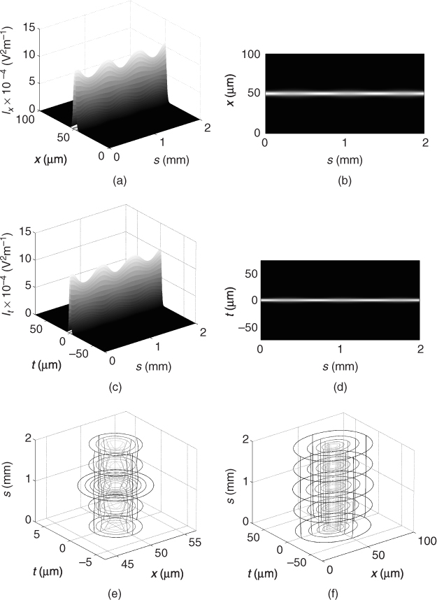
Figure 1.8a–c illustrates nematicon evolution for a given waist w0 and various powers P at the input: at low power (P = 0.1 mW, panel a) the beam diffracts. As power increases (P = 1 mW, panel b) a nematicon forms, with a long breathing period and large waist oscillations. Further increases in power (P = 2 mW, panel c) lead to shorter periods and smaller oscillations in the waist.
Figure 1.8 Beam evolution in the plane ts for w0 = 2.5 μm, λ = 632.8 nm, and (a) P = 0.1 mW; (b) P = 1 mW; (c) P = 2 mW. Gray maps of beam waist at (d) λ = 632.8 nm and (e) λ = 1064 nm against (Poynting) propagation coordinate s and input waist w0 for P = 0.5 mW, P = 1 mW and P = 3 mW, respectively. The units of colorbar legends are micrometers; here L = 100μm and θ0 = π/6.
For initial conditions corresponding to a point below the existence curve, the solitary wave initially increases the waist and undergoes slow and large oscillations. As the initial conditions approach the existence curve, the nematicon remains almost undistorted against propagation; it is worth noting that small changes persist as the exact soliton is not Gaussian (Fig. 1.8). As the initial conditions cross the existence curve, the nematicon breathes again, with both period and amplitude of oscillations related to the departure from the exact soliton. An aperiodic breathing appears for large oscillations, as the self-induced parabolic index well varies in propagation (see Eq. 1.27). Finally, Figure 1.8 also shows that self-confinement is eased at lower wavelengths.
1.4 Experimental Observations
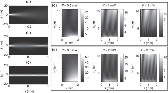
The typical setup for the observation of nematicons is sketched in Figure 1.9, which shows an optical microscope imaging, the light outscattered by the NLC as the beam propagates in a planar cell. In a planar cell, two glass plates are held parallel to one another by spacers at a distance of ![]() m (across x), with the inner surfaces treated by mechanical rubbing of a coating to induce the desired alignment of the molecules. A thin film of indium tin oxide (ITO) can also be predeposited on the plates for the application of an electric potential across the NLC thickness. Planar cells are normally filled by capillarity and glued together using the spacers. One (or two) other glass slide(s)—treated to ensure molecular anchoring, as well—is (are) arranged perpendicular to the cell (i.e., normal to z) in order to seal the entrance (and the exit) of the cell and prevent the formation of a meniscus with the consequent unpredictable depolarization of the input excitation. An optical microscope and a camera can image the light scattered by a beam out of one of the glass plates, thus allowing the real-time monitoring of the evolution of the excitation in the observation plane yz [1, 2, 47–49]. In cells with reduced propagation length (as compared to the attenuation distance) along z, the output profile can be acquired at the exit with a microscope objective and another camera [50–53]. At the input, a light beam linearly polarized in the plane containing the molecular director and the wave-vector, that is, an extraordinary wave, is focused with a microscope objective at the cell entrance, ensuring a transverse size and a direction of propagation suitable for the excitation of a self-trapped nematicon in the NLC bulk [54]. A weak copolarized collinear probe at a different wavelength can also be colaunched to monitor the formation of a waveguide and its signal transmission [48, 53].
m (across x), with the inner surfaces treated by mechanical rubbing of a coating to induce the desired alignment of the molecules. A thin film of indium tin oxide (ITO) can also be predeposited on the plates for the application of an electric potential across the NLC thickness. Planar cells are normally filled by capillarity and glued together using the spacers. One (or two) other glass slide(s)—treated to ensure molecular anchoring, as well—is (are) arranged perpendicular to the cell (i.e., normal to z) in order to seal the entrance (and the exit) of the cell and prevent the formation of a meniscus with the consequent unpredictable depolarization of the input excitation. An optical microscope and a camera can image the light scattered by a beam out of one of the glass plates, thus allowing the real-time monitoring of the evolution of the excitation in the observation plane yz [1, 2, 47–49]. In cells with reduced propagation length (as compared to the attenuation distance) along z, the output profile can be acquired at the exit with a microscope objective and another camera [50–53]. At the input, a light beam linearly polarized in the plane containing the molecular director and the wave-vector, that is, an extraordinary wave, is focused with a microscope objective at the cell entrance, ensuring a transverse size and a direction of propagation suitable for the excitation of a self-trapped nematicon in the NLC bulk [54]. A weak copolarized collinear probe at a different wavelength can also be colaunched to monitor the formation of a waveguide and its signal transmission [48, 53].
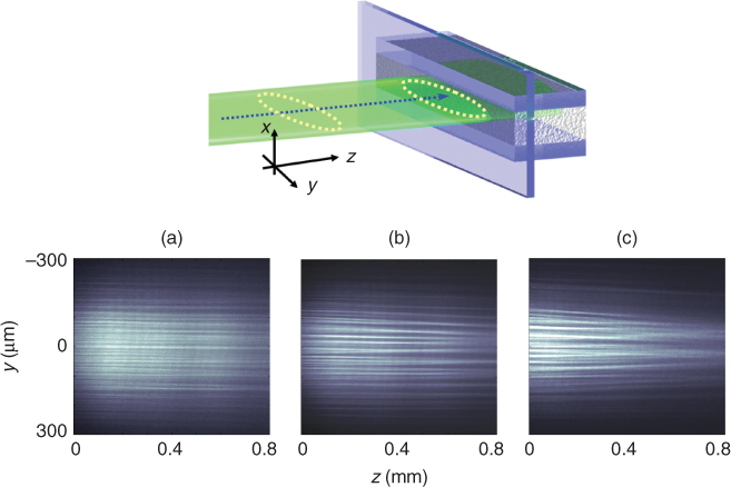
Figure 1.9 Typical experimental setup and planar cell, with copolarized collinear pump and probe launched in the NLC and propagating along z. The outscattered light at each wavelength is acquired with an optical microscope, a filter, and a camera, before digital processing.
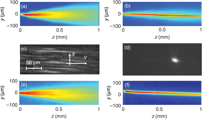
Figure 1.10 shows a set of photographs displaying a 2 mW Gaussian beam of waist w0 = 4 μm at λ = 514.5 nm propagating along a 100-μm -thick cell filled with the NLC mixture E7 and with director planarly oriented along z at the glass interfaces but pretilted in the xz plane by an external voltage across x (Fig. 1.3): for (ordinary) input polarization along y the beam diffracts, as its intensity cannot overcome the Freedericksz threshold (Fig. 1.10a); for (extraordinary) input polarization along x the beam undergoes self-focusing and becomes a spatial soliton, with an invariant profile over several Rayleigh lengths [3, 1, 2] (Fig. 1.10b). Figure 1.10c and d shows the corresponding output beam profiles after propagation over 1.5 mm in linear and solitary cases, respectively; the nematicon remains bell shaped and circularly symmetric despite the NLC anisotropy and the presence of boundaries across x. Similarly, a colaunched probe at 632.8 nm (its power is negligible with respect to the green beam) either diffracts when the nematicon is not excited, or gets confined in the nematicon waveguide despite its wavelength (Fig. 1.10e and f). The nonlocal character of the nematicon, in fact, allows light at longer wavelengths being trapped in the nematicon refractive potential [2, 48].
Figure 1.10 Behavior of light inside the NLC sample acquired through the setup shown in Figure 1.9. Ordinary (a) and extraordinary (b) propagation when the input power is 2 mW. The corresponding output beam profiles are shown in panels (c) and (d), for the ordinary and extraordinary wave, respectively. Propagation of an extraordinarily polarized red probe corresponding to the absence (e) and presence (f) of the soliton.
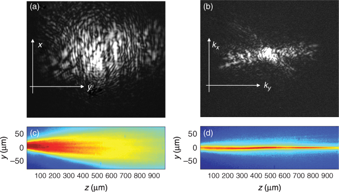
Taking advantage of the nonlocal response of NLC [35, 40, 49], nematicons can also be excited by spatially incoherent beams that are bell shaped with a speckle structure as obtained when a coherent beam is launched through a rotating diffuser. The nonlocality, in fact, acts as a low pass filter and allows the reorientational nonlinearity to respond according to the excitation envelope. Because the wave-vector spectrum is wider, however, a higher power is required to compensate the increased diffraction. Figure 1.11a shows the input profile of a speckled 514.5 nm beam generated with the aid of a diffuser and Figure 1.11b is the corresponding spatial spectrum; for an incoherent beam as in (a) and an input power of 2.7 mW in the same cell as in Figure 1.10, Figure 1.11c shows the diffraction in the y polarization (ordinary) and Figure 1.11d the nematicon in the x polarization (extraordinary) [47, 55, 56].
Figure 1.11 Speckled beam at the input of the NLC cell (a) and its spatial spectrum (b). Intensity distribution inside the sample for input polarizations corresponding to the ordinary (c) and extraordinary (d) component; input power is 2.7 mW.
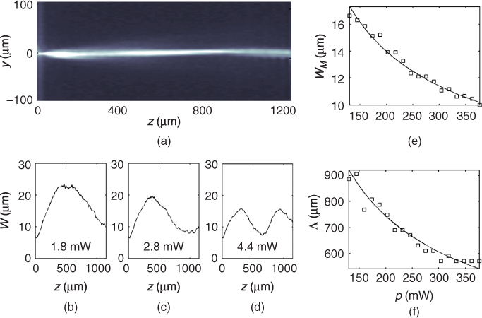
Nonlocal character of nematicons is demonstrated also by their breathing in propagation, as theoretically discussed in Section 1.2.2.1. Figure 1.12 shows experimental results obtained exciting the NLC E7 with an NIR beam (λ = 1064 nm). As predicted, beam width oscillates in a periodic manner in propagation, with both amplitude and period of oscillation decreasing with input power: in the plotted cases, diffraction prevails at the early stage, that is, we have w0 < ws for all range of used powers (Section 1.2.2.1) [40].
Figure 1.12 (a) Example of acquired intensity profile in plane yz. (b–d) Waist versus z. (e) Maximum waist and (f) breathing period versus input power (symbols are experimental data and solid lines are fits from theory).
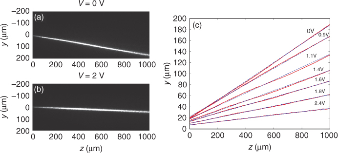
As the NLC behave as birefringent uniaxials, their optic axis coincides with the molecular director ![]() , and because all-optical reorientation and self-focusing are driven (below the Freedericksz threshold) by extraordinary waves, nematicons are subject to walk-off; that is, their Poynting vector is not collinear with the wave-vector but walks off at an angle. The latter depends on the angle θ and the dispersion, and can reach several degrees in NLC owing to the large birefringence [57]. A nematicon excited as discussed in the above examples, that is, with electric field linearly polarized in xz, experiences walk-off in the same plane and, if launched with wave-vector along z in the mid-plane x = 0, it travels out of it towards one of the glass plates, until it interacts with the (repulsive) boundaries. Therefore, a typical nematicon trajectory in a planar cell with a voltage bias is oscillating in xz, unless the walk-off is compensated for by an input wave-vector tilt. The role of walk-off is more apparent in planar cells with director in yz but at an angle with respect to z (Fig. 1.3 for ζ0 ≠ 0), in order to have noncollinear wave-vector and z axis. Let us consider a planar cell with director lying in yz but at π/4 with respect to
, and because all-optical reorientation and self-focusing are driven (below the Freedericksz threshold) by extraordinary waves, nematicons are subject to walk-off; that is, their Poynting vector is not collinear with the wave-vector but walks off at an angle. The latter depends on the angle θ and the dispersion, and can reach several degrees in NLC owing to the large birefringence [57]. A nematicon excited as discussed in the above examples, that is, with electric field linearly polarized in xz, experiences walk-off in the same plane and, if launched with wave-vector along z in the mid-plane x = 0, it travels out of it towards one of the glass plates, until it interacts with the (repulsive) boundaries. Therefore, a typical nematicon trajectory in a planar cell with a voltage bias is oscillating in xz, unless the walk-off is compensated for by an input wave-vector tilt. The role of walk-off is more apparent in planar cells with director in yz but at an angle with respect to z (Fig. 1.3 for ζ0 ≠ 0), in order to have noncollinear wave-vector and z axis. Let us consider a planar cell with director lying in yz but at π/4 with respect to ![]() for zero bias, that is, ζ0 = π/4: a nematicon launched by a y-polarized input beam with
for zero bias, that is, ζ0 = π/4: a nematicon launched by a y-polarized input beam with ![]() experiences a walk-off of about 8° at λ = 632.8 nm; hence, its Poynting vector is slanted with respect to
experiences a walk-off of about 8° at λ = 632.8 nm; hence, its Poynting vector is slanted with respect to ![]() , as visible in the observation plane yz and shown in the photograph Figure 1.13a and b [30].
, as visible in the observation plane yz and shown in the photograph Figure 1.13a and b [30].
Figure 1.13 Direct observation of nematicon walk-off. Extraordinary wave beam with 3 mW initial power propagating in a cell (a) with zero bias and (b) with 2V applied across the NLC layer. (c) Nematicon trajectories in the observation plane yz for several applied voltages; solid and dashed lines are measured paths and corresponding linear best-fits, respectively. Here, the wavelength is 632.8 nm.
The cell sketched in Figure 1.3 for ζ0 ≠ 0 can also be employed to alter the walk-off by applying a voltage across its thickness. The electro-optic NLC response can make the molecules reorientate out of the plane yz, correspondingly changing the principal plane (k,![]() ) where the Poynting vector lies; in the limit of a molecular director
) where the Poynting vector lies; in the limit of a molecular director ![]() , the extraordinary wave will take an ordinary configuration, that is, the walk-off angle goes to zero as the Poynting vector becomes collinear with the wave-vector. Therefore, the application of a bias across the thickness of this cell can progressively reduce the walk-off observable in yz and modify the nematicon direction of propagation in the NLC volume (Fig. 1.13c and Chapter 5) [30, 58]. Such an approach to nematicon steering, that is, one based on electro-optic changes in walk-off, is just an example of a variety of strategies that can be implemented to modify the trajectory of a spatial soliton (and its waveguide) and therefore route/readdress the guided signal(s) [59–62]. Several cases are discussed in this book, see, for example, Chapters 5, 6, 11 [43, 63–67]. Given their robustness, the path of spatial solitons in NLC can also be affected by mutual interactions between two (or more) of them, as briefly addressed in the following section.
, the extraordinary wave will take an ordinary configuration, that is, the walk-off angle goes to zero as the Poynting vector becomes collinear with the wave-vector. Therefore, the application of a bias across the thickness of this cell can progressively reduce the walk-off observable in yz and modify the nematicon direction of propagation in the NLC volume (Fig. 1.13c and Chapter 5) [30, 58]. Such an approach to nematicon steering, that is, one based on electro-optic changes in walk-off, is just an example of a variety of strategies that can be implemented to modify the trajectory of a spatial soliton (and its waveguide) and therefore route/readdress the guided signal(s) [59–62]. Several cases are discussed in this book, see, for example, Chapters 5, 6, 11 [43, 63–67]. Given their robustness, the path of spatial solitons in NLC can also be affected by mutual interactions between two (or more) of them, as briefly addressed in the following section.
1.4.1 Nematicon–Nematicon Interactions
Because NLC exhibits a large nonlocality, nematicons tend to behave as incoherent entities and, as pointed out above, they can also be excited by spatially incoherent excitations. Similarly, the interaction between two or more nematicons is essentially incoherent, that is, it largely depends on the interaction between the associated refractive index deformations or waveguides. In all cases, where the nonlocality range extends beyond the details of the field distribution, this interaction is attractive and two (or more) nematicons tend to get closer to one another as they propagate (see also Chapter 2) [68–71]. This concept is illustrated in Figure 1.14a–d showing the simulated attraction of two nematicons launched in plane yz at a relative angle of 2°: the refractive index perturbation (shown in Fig. 1.14b and c at the input and by the maximum separation, respectively) provides a transverse link between the two solitons, which attracts and bends their paths toward one another (Fig. 1.14d), eventually crossing and interlacing. The results of an actual experiment carried out in a biased cell with ζ0 = 0° at λ = 514.5 nm are displayed in Figure 1.14e–g for increasing input power, from 1.3 mW (e) to 1.7 mW (f) and 4.3 mW (g), respectively.
Figure 1.14 Mutual interaction between two solitons. Intensity profile at the input section (a) and the corresponding computed self-induced index landscape (b). (c) Refractive index distribution when the distance between solitons is maximum. (d) Interaction of numerically computed nematicons in the plane yz. Experimental interaction between nematicons for input power of 1.3 (e), 1.7 (f), and 4.3 mW (g). Wavelength is 514.5 nm.
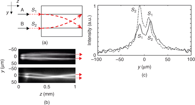
As not only the nematicons but also the transmitted signal(s) change trajectories when the interaction takes place, attraction between nematicons can be exploited to implement various analog or digital processors/routers, from power-driven switches to logic gates [72, 73]. Figure 1.15 is an example of excitation-dependent X-junction performing a power-controlled interchange of the output channels.
Figure 1.15 All-optical X-junction. Principle of the device: two nematicons (labeled as A and B) are launched inside the NLC cell with equal initial powers: if input power is small, the interaction is weak and no appreciable motion takes place in the light path, whereas for high power nonlinear interaction gives rise to mutual attraction, up to crossing and position exchange with respect to the initial configuration, thereby forming an X-junction. (a) Signals launched on light-induced guides A and B are indicated as S1 and S2, respectively. (b) Measured light distribution on the plane yz for an initial power of 1.73 mW (top panel) and 4.3 mW (bottom panel). (c) Scattered light distribution on the section z = 1 mm.
In the experiments shown in Figures 1.14 and 1.15 the actual motion of nematicons inside the samples are 3D, given the not null velocity along the x axis owing to walk-off (see the discussion for a single nematicon). To study pure planar interaction between nematicons, an unbiased cell with ζ0 ≠ 0 can be employed. To investigate the interaction of solitons we take the input beam in the form
1.34 
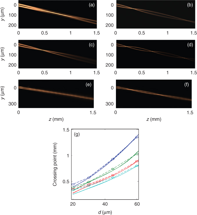
that is, two fundamental Gaussian beams launched in the mid-plane with wave-vectors parallel to ![]() and separated by d along y. Each beam carries the same power P and ϕ is the phase difference between them. We are interested in long-range interactions, that is, w0 much smaller than the initial separation d: in this limit, mutual interaction forces are independent from ϕ due to nonlocality, at variance with (local) Kerr media [13] (see Chapter 2). Figure 1.16a–d shows numerical simulations of λ = 1064 nm nematicons interacting: as the power increases, the attraction becomes stronger, giving rise to multiple crossings along propagation. For a better comparison with experiments the scattering losses were accounted for, yielding a decreasing attraction versus z. Figure 1.16e and f shows the corresponding data: as the input power increases, the attraction pulls more and more the beams toward each other, up to three crossings when P = 10 mW. Finally, Figure 1.16g displays the trend of the first crossing point versus initial separation d for several excitations: the attraction is larger for both closer beams and higher powers [71].
and separated by d along y. Each beam carries the same power P and ϕ is the phase difference between them. We are interested in long-range interactions, that is, w0 much smaller than the initial separation d: in this limit, mutual interaction forces are independent from ϕ due to nonlocality, at variance with (local) Kerr media [13] (see Chapter 2). Figure 1.16a–d shows numerical simulations of λ = 1064 nm nematicons interacting: as the power increases, the attraction becomes stronger, giving rise to multiple crossings along propagation. For a better comparison with experiments the scattering losses were accounted for, yielding a decreasing attraction versus z. Figure 1.16e and f shows the corresponding data: as the input power increases, the attraction pulls more and more the beams toward each other, up to three crossings when P = 10 mW. Finally, Figure 1.16g displays the trend of the first crossing point versus initial separation d for several excitations: the attraction is larger for both closer beams and higher powers [71].
Figure 1.16 Planar interactions between nematicons. Numerically calculated nematicon path for d = 25 μm and (a) P = 0.2, (b) 0.5, (c) 1, and (d) 3 mW. Actual nematicon trajectories for the same d and (e) P = 2 mW, (f) P = 10 mW. (g) Position of the first crossing versus d; solid (P = 0.7, 1, 1.3, 1.7 mW from top to bottom, respectively) and dashed lines with symbols (4, 6, 8, 10 mW from top) are calculated and experimental, respectively. Small discrepancies between theoretical and experimental power values can be ascribed to the 2D nature of the code (see Chapter 11). Here, w0 = 7 μm and θ0 = 45°.
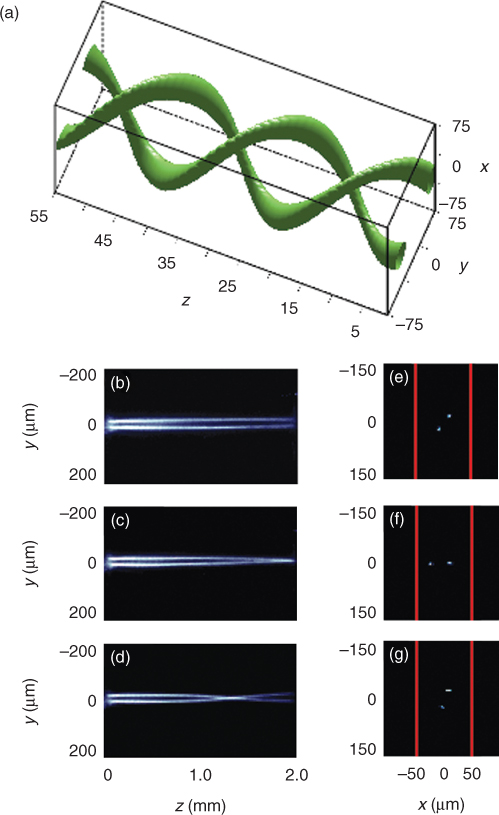
In a thick NLC cell, in general, the attractive interaction between nematicons is obviously not limited to the plane yz of observation. If two nematicons are launched skewed to one another with initial momenta out of yz, the mutual attraction can combine the two solitons in a dipolar structure with angular momentum, in such a way that the two-nematicon cluster rotates as it propagates down the cell, maintaining a constant profile as the centrifugal force is balanced by the nonlinear attraction [50, 52, 74]. The two nematicons will therefore spiral in a rigid manner around the straight trajectory of the center of mass as sketched in Figure 1.17a and their angular velocity will be dependent on the initial angular momentum, that is, components of the wave-vectors launched out of yz (i.e., ![]() ) and the effective masses associated to the input powers. Therefore, the position of the two spots at the output of the cell is dependent on the input powers, as visible in the experimental results shown in Figure 1.17b–g, obtained in a planar cell (unbiased) with molecular director at π/6 with respect to
) and the effective masses associated to the input powers. Therefore, the position of the two spots at the output of the cell is dependent on the input powers, as visible in the experimental results shown in Figure 1.17b–g, obtained in a planar cell (unbiased) with molecular director at π/6 with respect to ![]() in the plane yz (i.e., ζ0 = 30°). Each nematicon carries the same power and input wave-vectors are tilted in the plane yz, so that the Poynting vector of each beam is parallel to
in the plane yz (i.e., ζ0 = 30°). Each nematicon carries the same power and input wave-vectors are tilted in the plane yz, so that the Poynting vector of each beam is parallel to ![]() . Moreover, to avoid velocity drifts along x the wave-vector components along
. Moreover, to avoid velocity drifts along x the wave-vector components along ![]() are equal in modulus and opposite in sign. The rate of angular rotation of the nematicon cluster is proportional to the total excitation of the two identical solitons, as theoretically expected [52].
are equal in modulus and opposite in sign. The rate of angular rotation of the nematicon cluster is proportional to the total excitation of the two identical solitons, as theoretically expected [52].
Figure 1.17 (a) Artist's 3D sketch of spiraling nematicons. Measured (middle column) evolution in the plane yz and (right panels) corresponding output distribution in plane xy for initial powers of (b–e) 2.1, (c–f) 3.3, and (d–g) 3.9 mW. Here, the wavelength is λ = 1064 nm, the cell thickness is 100 μm, and the propagation length is 2 mm.
A special case of nonlinear incoherent interaction between the beams in NLC is the formation of a vector soliton, that is, a self-confined wave where diffraction is balanced by the combined intensities of two color components in the extraordinary polarization. If the power in each input beam is too low to excite a nematicon by itself but their coaction is sufficient to induce self-trapping, the two components are capable of spatially confining each other forming a vectorial nematicon, undergoing the weighted walk-off between the two colors, as dispersion can be significant and affect birefringence as well as diffraction. Figure 1.18 shows experimental results obtained in a planar (unbiased) NLC cell with molecular director anchored at π/4 with respect to ![]() in the plane yz (in other words ζ0 = π/4), with input wave-vector tilted such that the two Poynting vectors at the two different colors overlap; the two components were in the red at 632.8 nm and in the near-infrared at 1064 nm [44]. More in general, the simultaneous launch of two beams at different wavelength implies a reciprocal influence on the breathing in propagation, that is, the waist behavior versus z. Noticeably, the effect of each wavelength is different for three reasons: a diverse amount of diffraction, a different optical perturbation for a fixed intensity profile, and finally a different refractive index profile for a given reorientation angle, the last two are caused by dispersion in the birefringence.
in the plane yz (in other words ζ0 = π/4), with input wave-vector tilted such that the two Poynting vectors at the two different colors overlap; the two components were in the red at 632.8 nm and in the near-infrared at 1064 nm [44]. More in general, the simultaneous launch of two beams at different wavelength implies a reciprocal influence on the breathing in propagation, that is, the waist behavior versus z. Noticeably, the effect of each wavelength is different for three reasons: a diverse amount of diffraction, a different optical perturbation for a fixed intensity profile, and finally a different refractive index profile for a given reorientation angle, the last two are caused by dispersion in the birefringence.
Figure 1.18 (Left) Acquired and (right) calculated evolution of the red beam component in the plane st. (a and b) A 0.1 mW red beam at 632.8 nm is colaunched with a 1.2 mW near-infrared beam; (c and d) a 0.4 mW red beam is injected by itself; (e and f) 0.4 mW red and 1.2 mW infrared beams are colaunched and a vector nematicon is generated. Both beams are extraordinary waves with comparable Rayleigh lengths. Calculations were carried out for in-coupling efficiencies of 40% and 62% for red and near-infrared, respectively.
1.4.2 Modulational Instability
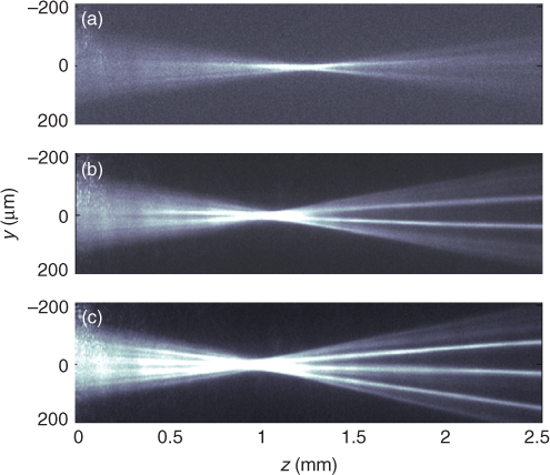
As anticipated in Section 1.2.1.2, transverse patterns with a dominant harmonic component in space can emerge in the propagation of a wide beam in a self-focusing reorientational medium and in the presence of nonlocality [75, 76]. Nonlocal modulational instability can indeed be observed in NLC, both in the spontaneous case originating from noise [41] and in the "seeded" case in the presence of an input (transverse) modulation [77, 78]. Modulational instability can be investigated versus propagation distance and versus input power, eventually resulting in a number of filaments or solitary waves emerging from the wide input beam. Figure 1.19 shows typical results in a planar NLC cell with a bias V = 1.6V, using a highly elliptical input beam at 514.5 nm: the transverse modulation is clearly visible in the plane yz for an input power of 17 mW (Fig. 1.19a), but gets more and more pronounced at 88 mW with the emergence of filaments (Fig. 1.19b); at 193 mW the nematicons attract one another and the whole cluster deforms undergoing “global” self-focus (Fig. 1.19c) [41, 42, 79].
Figure 1.19 Sketch of the experiment on modulational instability, and pictures of the emerging pattern in yz for an input power of (a) 17 mW, (b) 88 mW, and (c) 193 mW.
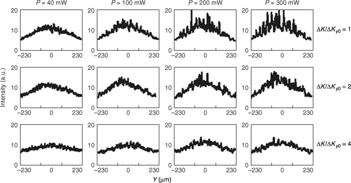
In analogy with nematicons of which is considered a precursor, modulational instability can also be generated with a spatially incoherent beam at the expense of the gain, with a resulting path contrast which at a given propagation distance is dependent on the spatial spectrum and on the excitation, as apparent in Figure 1.20 [80]. Owing to the larger diffraction counteracting nonlinear self-focusing, amplification of high frequencies is weakened as beam incoherence increases. Modulational instability patterns and/or clusters of nematicons can even be steered in the direction of propagation by modifying the walk-off with a voltage bias, that is, by changing the principal plane of propagation [30].
Figure 1.20 Synopsis of experimental results on modulational instability for various degrees of incoherence (ratio ΔK/ΔKy0 between the incoherent and a coherent spatial spectrum) and input power. The graphs show the transverse pattern after propagation along z for 200 μm.
While the model discussed in Section 1.2.1.2 is valid in the early stages of propagation when the perturbations are actually small, as solitons begin to emerge (Fig. 1.19b) their mutual interactions become relevant and need to be accounted for (Fig. 1.19c). In this regime, a large number of solitons can be represented as a gas of interacting particles that are capable of undergoing clustering and dynamic phase transitions [81].
The generation of multiple solitons from a wide beam can be enhanced by imposing a phasefront curvature on the input beam. In fact, by tailoring the size of a converging (focused) input beam, modulational instability can trigger the generation of multiple nematicons from the focal point, as, for example, shown in Figure 1.21 [82]. The number of nematicons increases with an increase in power, whereas their exact location depends on noise-induced fluctuations.
Figure 1.21 Generation of multiple nematicons from a focused input beam at 1064 nm in a planar NLC cell for various input powers: (a) 5 mW, (b) 30 mW, and (c) 47.5 mW.
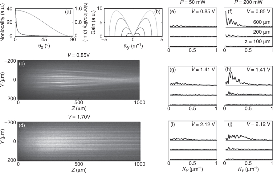
Modulational instability in biased NLC cells with ζ0 = 0 can also be employed to investigate the interplay between nonlocality and nonlinearity, theoretically discussed in Section 1.2.1.1. As the voltage applied to the cell increases, both nonlinearity ![]() (Eq. 1.6) and nonlocality l (Eq. 1.4) decrease. This is included in Equation 1.15, which predicts that the nonlinear gain reduces in both peak and bandwidth as α (inversely proportional to nonlocality) goes up (Fig. 1.22). On physical grounds, nonlocality effectively acts as an integrator and therefore, filters out the response at high spatial frequencies. Figure 1.22 shows some experimental results: the modulational instability gain spectrum lowers in peak and bandwidth (in wave-vector space) at higher voltages [36].
(Eq. 1.6) and nonlocality l (Eq. 1.4) decrease. This is included in Equation 1.15, which predicts that the nonlinear gain reduces in both peak and bandwidth as α (inversely proportional to nonlocality) goes up (Fig. 1.22). On physical grounds, nonlocality effectively acts as an integrator and therefore, filters out the response at high spatial frequencies. Figure 1.22 shows some experimental results: the modulational instability gain spectrum lowers in peak and bandwidth (in wave-vector space) at higher voltages [36].
Figure 1.22 Calculated (a) trend of nonlocality (black line) and nonlinearity (gray line) versus θ0 and (b) gain versus transverse wave-vector ky for α = 0.001, 0.1, 1, 10, 100 from top to bottom, respectively. The gain is computed for ![]() . Light intensity in plane yz when a 150 mW elliptic Gaussian beam is launched in the cell with ζ0 = 0 and bias (c) 0.85 V and (d) 1.70 V. Measured spectral gain (in three longitudinal sections as marked) versus wave-vector ky for input power (e,g,i) 50 mW or (f,h,j) 200 mW and voltages as indicated. Here, the wavelength is 1064 nm and the NLC thickness is 100 μm.
. Light intensity in plane yz when a 150 mW elliptic Gaussian beam is launched in the cell with ζ0 = 0 and bias (c) 0.85 V and (d) 1.70 V. Measured spectral gain (in three longitudinal sections as marked) versus wave-vector ky for input power (e,g,i) 50 mW or (f,h,j) 200 mW and voltages as indicated. Here, the wavelength is 1064 nm and the NLC thickness is 100 μm.
1.5 Conclusions
In this chapter, we tried to provide a brief (and incomplete) overview of the basic features of (bright) optical spatial solitons in NLC, touching upon pertinent models, numerics, and experiments in an attempt to stimulate the interest of the readers and encourage them to look up the growing literature and the following chapters of this book.
Acknowledgments
We wish to express our gratitude to all those who have contributed to the work presented in this chapter, in particular, to Marco Peccianti, Claudio Conti, and Cesare Umeton. A.A. thanks Regione Lazio for the financial support provided.
1. G. Assanto, M. Peccianti, and C. Conti. Nematicons: Optical spatial solitons in nematic liquid crystals. Opt. Photon. News, 14(2):44–48, 2003.
2. M. Peccianti, G. Assanto, A. De Luca, C. Umeton, and I. C. Khoo. Electrically assisted self-confinement and waveguiding in planar nematic liquid crystal cells. Appl. Phys. Lett., 77(1):7–9, 2000.
3. P. G. DeGennes and J. Prost. The Physics of Liquid Crystals. Oxford Science, New York, 1993.
4. I. C. Khoo. Liquid Crystals: Physical Properties and Nonlinear Optical Phenomena. Wiley, New York, 1995.
5. F. Simoni. Nonlinear Optical Properties of Liquid Crystals. World Scientific, Singapore, 1997.
6. I. C. Khoo. Nonlinear optics of liquid crystalline materials. Phys. Rep., 471:221–267, 2009.
7. I. C. Khoo. Extreme nonlinear optics of nematic liquid crystals. J. Opt. Soc. Am. B, 471:221–267, 2009.
8. G. K. L. Wong and Y. R. Shen. Optical-field-induced ordering in the isotropic phase of a nematic liquid crystal. Phys. Rev. Lett., 30:895, 1973.
9. D. Paparo, L. Marrucci, G. Abbate, E. Santamato, M. Kreuzer, P. Lehnert, and T. Vogeler. Molecular-field-enhanced optical kerr effect in absorbing liquids. Phys. Rev. Lett., 78:38–41, 1997.
10. I. Janossy, A. D. Lloyd, and B. S. Wherrett. Anomalous optical Freedericksz transition in an absorbing liquid crystal. Mol. Cryst. Liq. Cryst., 179:1–12, 1990.
11. R. Y. Chiao, E. Garmire, and C. H. Townes. Self-trapping of optical beams. Phys. Rev. Lett., 13(15):479–482, 1964.
12. P. L. Kelley. Self-focusing of optical beams. Phys. Rev. Lett., 15(26):1005–1008, 1965.
13. G. I. Stegeman and M. Segev. Optical spatial solitons and their interactions: Universality and Diversity. Science, 286(5444):1518–1523, 1999.
14. G. Baruch, S. Maneuf, and C. Froehly. Propagation soliton et auto-confinement de faisceaux laser par non linearite optique de Kerr. Opt. Commun., 55:201, 1985.
15. J. E. Bjorkholm and A. A. Ashkin. cw self-focusing and self-trapping of light in sodium vapor. Phys. Rev. Lett., 32(4):129–132, 1974.
16. G. C. Duree, J. L. Shultz, G. J. Salamo, M. Segev, A. Yariv, B. Crosignani, P. Di Porto, E. J. Sharp, and R. R. Neurgaonkar. Observation of self-trapping of an optical beam due to the photorefractive effect. Phys. Rev. Lett., 71(4):533–536, 1993.
17. S. Tzortzakis, L. Sudrie, M. Franco, B. Prade, A. Mysyrowicz, A. Couairon, and L. Bergé. Self-guided propagation of ultrashort IR laser pulses in fused silica. Phys. Rev. Lett., 87(21):213902, 2001.
18. A. Fratalocchi, G. Assanto, K. A. Brzdakiewicz, and M. A. Karpierz. Discrete propagation and spatial solitons in nematic liquid crystals. Opt. Lett., 29(13):1530–1532, 2004.
19. F. Lederer, G. I. Stegeman, D. N. Christodoulides, G. Assanto, M. Segev, and Y. Silberberg. Discrete solitons in optics. Phys. Rep., 463(1–3):1–126, 2008.
20. O. Bang, W. Krolikowski, J. Wyller, and J. J. Rasmussen. Collapse arrest and soliton stabilization in nonlocal nonlinear media. Phys. Rev. E, 66:046619, 2002.
21. Y. S. Kivshar and G. P. Agrawal. Optical Solitons. Academic, San Diego, CA, 2003.
22. B. Y. Zeldovich, N. F. Pilipetskii, A. V. Sukhov, and N. V. Tabiryan. Giant optical nonlinearity in the mesophase of a nematic liquid crystals (nlc). JETP Letters, 31:263–269, 1980.
23. S. D. Durbin, S. M. Arakelian, and Y. R. Shen. Optical-field-induced birefringence and Freedericksz transition in a nematic liquid crystal. Phys. Rev. Lett., 47:1411–1414, 1981.
24. S. D. Durbin, S. M. Arakelian, and Y. R. Shen. Laser-induced diffraction rings from a nematic-liquid-crystal film. Opt. Lett., 6(9):411–413, 1981.
25. E. Braun, L. P. Faucheux, and A. Libchaber. Strong self-focusing in nematic liquid crystals. Phys. Rev. A, 48(1):611–622, Jul 1993.
26. D. W. McLaughlin, D. J. Muraki, M. J. Shelley, and X. Wang. A paraxial model for optical self-focussing in a nematic liquid crystal. Physica D, 88(1):55–81, 1995.
27. D. W. McLaughlin, D. J. Muraki, and M. J. Shelley. Self-focussed optical structures in a nematic liquid crystal. Physica D, 97(4):471–497, 1996.
28. F. Derrien, J. F. Henninot, M. Warenghem, and G. Abbate. A thermal (2D + 1) spatial optical soliton in a dye doped liquid crystal. J. Opt. A: Pure Appl. Opt., 2:332, 2000.
29. M. Warenghem, J. F. Blach, and J. F. Henninot. Thermo-nematicon: an unnatural coexistence of solitons in liquid crystals? J. Opt. Soc. Am. B, 25:1882–1887, 2008.
30. M. Peccianti, C. Conti, G. Assanto, A. De Luca, and C. Umeton. Routing of anisotropic spatial solitons and modulational instability in nematic liquid crystals. Nature, 432:733, 2004.
31. M. A. Karpierz. Solitary waves in liquid crystalline waveguides. Phys. Rev. E, 66(3):036603, 2002.
32. A. Fratalocchi, G. Assanto, K. Brzdakiewicz, and M. A. Karpierz. Discrete light propagation and self-trapping in liquid crystals. Opt. Express, 13(6):1808–1815, 2005.
33. U. A. Laudyn, M. Kwasny, and M. A. Karpierz. Nematicons in chiral nematic liquid crystals. Appl. Phys. Lett., 94(9):091110, 2009.
34. U. A. Laudyn, M. Kwasny, K. Jaworowicz, K. A. Rutkowska, M. A. Karpierz, and G. Assanto. Nematicons in twisted liquid crystals. Photon. Lett. Pol., 1(1):7, 2009.
35. C. Conti, M. Peccianti, and G. Assanto. Route to nonlocality and observation of accessible solitons. Phys. Rev. Lett., 91:073901, 2003.
36. M. Peccianti, C. Conti, and G. Assanto. The interplay between non locality and nonlinearity in nematic liquid crystals. Opt. Lett., 30:415, 2005.
37. I. A. Kol'chugina, V. A. Mironov, and A. M. Sergeev. On the structure of stationary solitons in systems with nonlocal nonlinearity. JETP Letters, 31(6):333–7, 1980.
38. A. W. Snyder and D. J. Mitchell. Accessible solitons. Science, 276:1538, 1997.
39. G. Assanto and G. Stegeman. Simple physics of quadratic spatial solitons. Opt. Express, 10(9):388–396, 2002.
40. C. Conti, M. Peccianti, and G. Assanto. Observation of optical spatial solitons in a highly nonlocal medium. Phys. Rev. Lett., 92:113902, 2004.
41. M. Peccianti, C. Conti, and G. Assanto. Observation of optical modulational instability in a non-local medium. Phys. Rev. E, 68:025602(R), 2003.
42. C. Conti, M. Peccianti, and G. Assanto. Spatial solitons and modulational instability in the presence of large birefringence: the case of highly non-local liquid crystals. Phys. Rev. E, 72:066614, 2005.
43. A. Alberucci and G. Assanto. Nonparaxial (1 + 1)D spatial solitons in uniaxial media. Opt. Lett., 36(2):193–195, Jan 2011.
44. A. Alberucci, M. Peccianti, G. Assanto, A. Dyadyusha, and M. Kaczmarek. Two-color vector solitons in nonlocal media. Phys. Rev. Lett., 97:153903, 2006.
45. A. Messiah. Quantum Mechanics. Dover Publications, New York, 1999.
46. A. Alberucci and G. Assanto. Dissipative self-confined optical beams in doped nematic liquid crystals. J. Nonlin. Opt. Phys. Mater., 16(3):295–305, 2007.
47. M. Peccianti and G. Assanto. Incoherent spatial solitary waves in nematic liquid crystals. Opt. Lett., 26:1791, 2001.
48. M. Peccianti and G. Assanto. Signal readdressing by steering of spatial solitons in bulk nematic liquid crystals. Opt. Lett., 26(21):1690–1692, 2001.
49. M. Peccianti, C. Conti, G. Assanto, A. De Luca, and C. Umeton. Nonlocal optical propagation in nonlinear nematic liquid crystals. J. Nonlin. Opt. Phys. Mater., 12:525, 2003.
50. A. Fratalocchi, A. Piccardi, M. Peccianti, and G. Assanto. Nonlinearly controlled angular momentum of soliton clusters. Opt. Lett., 32:1447, 2007.
51. A. Alberucci, M. Peccianti, and G. Assanto. Nonlinear bouncing of nonlocal spatial solitons at the boundaries. Opt. Lett., 32(19):2795–2797, 2007.
52. A. Fratalocchi, A. Piccardi, M. Peccianti, and G. Assanto. Nonlinear management of the angular momentum of soliton clusters: Theory and experiment. Phys. Rev. A, 75(6):063835, 2007.
53. Y. V. Izdebskaya, A. S. Desyatnikov, G. Assanto, and Y. S. Kivshar. Multimode nematicon waveguides. Opt. Lett., 36(2):184–186, 2011.
54. G. Assanto and M. Peccianti. Spatial solitons in nematic liquid crystals. IEEE J. Quantum Electron., 39:13–21, 2003.
55. M. Peccianti and G. Assanto. Nematic liquid crystals: a suitable medium for self-confinement of coherent and incoherent light. Phys. Rev. E, 65:035603(R), 2002.
56. K. G. Makris, H. Sarkissian, D. N. Christodoulides, and G. Assanto. Non local incoherent spatial solitons in liquid crystals. J. Opt. Soc. Am. B., 22 (7):1371–1377, 2005.
57. M. Peccianti, A. Fratalocchi, and G. Assanto. Transverse dynamics of nematicons. Opt. Express, 12:6524, 2004.
58. A. Alberucci, M. Peccianti, G. Assanto, G. Coschignano, A. De Luca, and C. Umeton. Self-healing generation of spatial solitons in liquid crystals. Opt. Lett., 30:1381–1383, 2005.
59. G. Assanto and M. Peccianti. Routing light at will. J. Nonlin. Opt. Phys. Mater., 16 (1):37–48, 2007.
60. G. Assanto, C. Umeton, M. Peccianti, and A. Alberucci. Nematicons and their angular steering. J. Nonlin. Opt. Phys. Mater., 15(1):33–42, 2006.
61. G. Assanto and M. Peccianti. Guiding and routing light with nematicons. Mol. Cryst. Liq. Cryst., 488:163–178, 2008.
62. G. Assanto, A. Alberucci, and A. Piccardi. Transverse self-acceleration of nematicons: can a self-confined beam change its own path? J. Nonlin. Opt. Phys. Mater., 20(3):237–242, 2011.
63. A. Piccardi, G. Assanto, L. Lucchetti, and F. Simoni. All-optical steering of soliton waveguides in dye-doped liquid crystals. Appl. Phys. Lett., 93:171104, 2008.
64. A. Piccardi, M. Peccianti, G. Assanto, A. Dyadyusha, and M. Kaczmarek. Voltage-driven in-plane steering of nematicons. Appl. Phys. Lett., 94(9):091106, 2009.
65. A. Alberucci, A. Piccardi, U. Bortolozzo, S. Residori, and G. Assanto. Nematicon all-optical control in liquid crystal light valves. Opt. Lett., 35(3):390–392, 2010.
66. A. Piccardi, A. Alberucci, and G. Assanto. Power-dependent nematicon steering via walk-off. J. Opt. Soc. Am. B, 27:2398–2404, 2010.
67. R. Barboza, A. Alberucci, and G. Assanto. Large electro-optic beam steering with nematicons. Opt. Lett., 36(14):2725–2727, 2011.
68. M. Peccianti, K. Brzadkiewicz, and G. Assanto. Nonlocal spatial soliton interactions in nematic liquid crystals. Opt. Lett., 27:1460, 2002.
69. W. Hu, T. Zhang, Q. Guo, L. Xuan, and S. Lan. Nonlocality-controlled interaction of spatial solitons in nematic liquid crystals. Appl. Phys. Lett., 89(7):071111, 2006.
70. Y. V. Izdebskaya, V. Shvedov, A. S. Desyatnikov, Y. S. Kivshar, W. Krolikowski, and G. Assanto. Incoherent interaction of nematicons in bias-free liquid crystal cells. J. Eur. Opt. Soc., 5:10008, 2008.
71. M. Kwasny, A. Piccardi, A. Alberucci, M. Peccianti, M. Kaczmarek, M. Karpierz, and G. Assanto. Nematicon-nematicon interactions in a medium with tunable nonlinearity and fixed nonlocality. Opt. Lett., 36 (13)(1):2566–2568, 2011.
72. M. Peccianti, C. Conti, G. Assanto, A. De Luca, and C. Umeton. All optical switching and logic gating with spatial solitons in liquid crystals. Appl. Phys. Lett., 81:3335, 2002.
73. A. Piccardi, A. Alberucci, U. Bortolozzo, S. Residori, and G. Assanto. Readdressable interconnects with spatial soliton waveguides in liquid crystal light valves. IEEE Photon. Technol. Lett., 22:694–696, 2010.
74. G. Assanto, N. F. Smyth, and A. L. Worthy. Two colour, nonlocal vector solitary waves with angular momentum in nematic liquid crystals. Phys. Rev. A, 78(1):013832, 2008.
75. W. Krolikowski, O. Bang, J. J. Rasmussen, and J. Wyller. Modulational instability in nonlocal nonlinear Kerr media. Phys. Rev. E, 64:016612, 2001.
76. J. Wyller, W. Krolikowski, O. Bang, and J. J. Rasmussen. Generic features of modulational instability in nonlocal Kerr media. Phys. Rev. E, 66:066615, 2002.
77. J. Beeckman, X. Hutsebaut, M. Haelterman, and K. Neyts. Induced modulation instability and recurrence in nematic liquid crystals. Opt. Express, 15:11185–11195, 2007.
78. J. Beeckman, K. Neyts, and M. Haelterman. Induced modulation instability and recurrence in nonlocal nonlinear media. J. Phys. B: At. Mol. Opt. Phys., 41:065402, 2008.
79. C. Conti, M. Peccianti, and G. Assanto. Complex dynamics and configurational entropy of spatial optical solitons in nonlocal media. Opt. Lett., 31(13):2030–2032, 2006.
80. M. Peccianti, C. Conti, E. Alberici, and G. Assanto. Spatially incoherent modulational instability in a nonlocal medium. Laser Phys. Lett., 2:25, 2005.
81. C. Conti. Complex light: Dynamic phase transitions of a light beam in a nonlinear nonlocal disordered medium. Phys. Rev. E, 72:066620, 2005.
82. M. Peccianti, C. Conti, and G. Assanto. Optical multisoliton generation in nematic liquid crystals. Opt. Lett., 28(22):2231–2233, 2003.