
Chapter 13: Time Dependence of Spatial Solitons in Nematic Liquid Crystals
Department of Electronics and Information Systems, Ghent University, Ghent, Belgium
13.1 Introduction
Although quite a number of applications of spatial solitons can be envisaged, the main application is their use as a dynamic optical interconnection. Depending on the speed at which the optical interconnection can be redirected from one output to another, different possibilities arise. If the switching time is in the order of a second, then typically only reconfigurable interconnects are possible, for example, protective switching (when one optical path fails, the optical signal is switched to a backup optical path). More interesting is the use as high-speed optical modulators, but then typically switching times in the order of a nanosecond are necessary. It is clear that the switching speed will determine for which application solitons can be of practical use, but in general one can state: the faster the switching speed, the better.
In this chapter, when we speak about switching time, we refer to the time it takes for the soliton to form when the optical beam is switched on. For applications as reconfigurable interconnects, the switching time is actually the time it takes to switch the optical signal from one output to another, but as this is much harder to describe theoretically, we stick to the simpler problem of switching on (or off) the soliton beam. Obviously, the temporal behavior of the soliton will be determined by the optical nonlinearity used for the soliton formation and different nonlinearities are important in liquid crystals with completely different typical timescales. Therefore, in the first part of this chapter, we give an overview of the behavior of the two most important optical nonlinearities in liquid crystals, namely, the reorientational and the thermal nonlinearity. The other nonlinearities are summarized briefly. In the second part, results for the soliton formation time are presented for the reorientational nonlinearity.
13.2 Temporal Behavior of Different Nonlinearities and Governing Equations
13.2.1 Reorientational Nonlinearity
The reorientational nonlinearity occurs because the liquid crystal director orients in order to decrease the total free energy of the system. Let us suppose that the system is in equilibrium, with no static or optical fields present. When switching on an electric field, the system will try to minimize its energy according to this novel situation, leading to director reorientation. This process is governed on one hand by the driving force (the electric field) and on the other hand by a counteracting force originating from the viscosity of the material. In general, the free energy of the liquid crystal consists of different terms:
13.1 ![]()
In this equation, K1, K2, and K3 are the elastic constants for splay, twist, and bend, respectively. q is a parameter that is zero for liquid crystals that align uniformly, whereas it is nonzero for chiral nematics that orient spontaneously in a twisted way.
13.2 ![]()
13.3 ![]()
Any change in time of the energy terms listed earlier will result in a reaction of the liquid crystal (LC) in order to minimize the energy in the new situation. This reaction will take a certain time. In the case that a reorientation of the director is necessary to reach the new equilibrium orientation, the time evolution is almost entirely due to the viscous forces in the anisotropic fluid and not to inertia of the molecules. The calculation of the reorientation in time is governed by the time-dependent version of the Euler–Lagrange equation:
In this equation, xi denotes the three spatial coordinates x, y, and z and summation is necessary over repeated indices. The angle θ is the inclination of the director. In the general case, one can also define a similar equation for the azimuthal angle ϕ. To shorten the notation, we will further denote a derivative ∂/∂xi as a subscript, i. This equation is derived from the theory of Ericksen and Leslie [1, 2] and contains the Rayleigh dissipation function ![]() for an anisotropic fluid, which basically describes the rate of viscous dissipation per unit volume. The Rayleigh dissipation function is given by Ericksen and Leslie [1]:
for an anisotropic fluid, which basically describes the rate of viscous dissipation per unit volume. The Rayleigh dissipation function is given by Ericksen and Leslie [1]:
13.5 
In the latter equation, the standard summation convention over repeating indices has to be enforced. ni indicate the components of the director, ui are the fluid velocities in different directions, and αi are the Leslie viscosity coefficients. The Leslie coefficients are not independent as α2 + α3 = α6 − α5. The Rayleigh dissipation function contains the rate of strain tensor
13.6 ![]()
and the angular velocity of the director relative to the fluid
13.7 ![]()
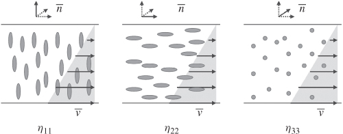
Different coefficients for the viscosity exist and the Leslie coefficients are related to the Miesowicz viscosities in the following way [3]: 2η1 = − α2 + α4 + α5, 2η2 = α2 + 2α3 + α4 − α5, η3 = α4/2, η12 = α1, and γ1 = α3 − α2. These Miesowicz coefficients are important because their physical meaning can be easily understood. Moreover, they can be measured experimentally. They express the viscosity of the liquid crystal during shear flow when the orientation of the director is kept constant [4, 5]. The meaning of the first three coefficients is explained in Figure 13.1. The physical meaning of coefficient η12 is more difficult to visualize. The first three Miesowicz coefficients are related to the force that is necessary to move the upper plate at a certain speed. This force will be different for the different orientations of the liquid crystal. In practice, it is difficult to keep the alignment of the liquid crystal fixed during the shear flow, so typically strong magnetic fields are used to maintain the alignment of the liquid crystal constant [6, 7]. Different methods exist to measure the different viscosity terms, and an overview can be found in Reference 8. The most important coefficient, however, is γ1, which is referred to as the rotational viscosity because it is related to the viscosity of rotation of the molecules around their axes. It characterizes the viscous torque associated with the angular velocity of the director. The switching times of liquid crystals in displays or other applications such as soliton generation are mainly determined by this rotational viscosity. For this reason, a large amount of publications have dealt with the measurement of this coefficient. A straightforward way of measuring this coefficient is by measuring the torque exerted on a sample by n̄ rotating with a constant angular velocity [9]. A simpler method is to derive γ1 from the switching and/or relaxation time in a planar cell when applying electric or magnetic fields. The switching time is approximately proportional to γ1d2 with d the thickness of the cell (Eq. 13.20). The behavior of the liquid crystal can then be easily observed under an optical polarization microscope [10, 11].
Figure 13.1 Director orientation according to which the coefficients η1, η2, and η3 are defined.
In most cases, when switching of the liquid crystal does not occur very fast, the flow of the liquid crystal material can be neglected (i.e., velocities ui are zero). When the flow cannot be neglected, an additional set of equations is necessary to calculate the temporal behavior of the liquid crystal, namely, the Navier–Stokes equations for an anisotropic fluid, given by:
13.8 ![]()
The first term includes the density of the fluid ρ and describes the inertia of the system. This term can often be neglected, and this approximation is known as the Berreman/van Doorn simplification. Fi refers to external body forces, and also this term can be neglected as mentioned before. The only term remaining contains the derivative of the dynamic stress tensor σji, which can be found from the Rayleigh dissipation function:
13.9 ![]()
In order to study the temporal dynamics of the system, one thus has to solve Equation 13.4 and σji, j = 0 simultaneously.
Let us now consider the case of flow not occurring; then the dissipation function reduces to:
13.2.2 Thermal Nonlinearity
As explained in the previous section, the thermal nonlinearity in liquid crystals mainly arises from order parameter changes that are related to the local temperature changes of the liquid crystal (Chapter 9). Let us suppose that a beam with certain intensity profile I(x, y) is launched into the liquid crystal and that diffraction can be neglected. Owing to absorption, the intensity will decrease exponentially along the propagation direction: ![]() . The heat dissipated in the material per unit volume P(x, y, z) because of absorption of the light is then simply given by αI(x, y, z).
. The heat dissipated in the material per unit volume P(x, y, z) because of absorption of the light is then simply given by αI(x, y, z).
The dynamic temperature distribution T due to heat dissipation in a material is governed by two constants: the specific heat capacity CV and the thermal conductivity k. The heat capacity describes the amount of heat per unit mass that is necessary to increase the temperature by one degree, whereas the heat conductivity expresses the material ability to conduct heat. The equation that describes the temperature variation when a certain power P is dissipated is given by:
Let us first consider a special case, assuming that the intensity profile has rotational symmetry in the xy plane and that the heat dissipation at z = 0 is given by αI(r), with r the radial distance from the origin. If the beam profile extends over a certain distance x0, then the heat conduction, governed by the first term in Equation 13.11, can be neglected if we consider timescales shorter than τ, for which
13.12 ![]()
The heat equation then reduces to:
13.13 ![]()
The temperature has the same profile as the heat dissipation as it cannot spread through conduction and the temperature increases linearly in time. Considering typical values for liquid crystals: ρ ≈ 103 kg/m3, CV ≈ 2.5 × 10³ J/(kgK)3 [12], k = 0.14 W/(mK) [13], and a beam waist of 3 μm, this regime is only valid for a value τ ![]() 160 μs. For a Gaussian beam with a total optical power Popt, the temperature variation at the beam center is then:
160 μs. For a Gaussian beam with a total optical power Popt, the temperature variation at the beam center is then:
13.14 ![]()
In order to calculate the temperature evolution for longer timescales, the heat equation reformulated in cylindrical coordinates is given by:
We can assume that the optical properties react almost instantaneously to temperature variations, which means that the temporal evolution of thermal solitons is governed by Equation 13.15. The mathematical solution of this equation is handled in different books and articles for different inputs and boundary conditions [14–16], so we will not further elaborate it. It is interesting to note that, for laser pulses with a duration smaller than τ, the heat profile and thus the refractive index profile are local during the duration of the pulse, after which the profiles spread and attenuate. Longer pulses will give rise to a large nonlocality, the width of which is mainly determined by the boundary conditions. These boundary conditions determine how the heat flows out of the geometry, typically either convectively or conductively.
13.2.3 Other Nonlinearities
Liquid crystals exhibit a number of optical nonlinearities that are not present in other material systems, such as the collective molecular reorientation in the nematic phase and the high thermal nonlinearity due to the changes in order parameter. Other nonlinearities such as the pure electronic nonlinearities (Chapter 14) can also be found in other materials. Up to now, soliton generation has been demonstrated with reorientational nonlinearities in the nematic phase ([17], see also Chapter 1), with thermal nonlinearities ([18], see also Chapter 9), and with photosensitive azobenzene liquid crystals [19]. Light bullets have been demonstrated by including electronic nonlinearities also [20]. All these nonlinearities have their own characteristic response times. For most of the effects, the switching-on time is dependent on the driving force, that is, the magnitude of the optical electric field or the optical power. This means that one can utilize a so-called overdriving scheme that is used also in liquid crystal displays: initially, a strong electric is applied to achieve a rapid initial response, after which the (lower) electric field is applied with a value that corresponds to the necessary condition to excite, for example, a stable soliton. Consequently, it is not the switching-on time that determines the speed of the system but the switching-off time. Table 13.1 shows the different response times in terms of the switching-off times for different optical nonlinearities in liquid crystals. Obviously, the electronic nonlinearities are the fastest as they are related directly to the behavior of the electron wave functions.
Table 13.1 Typical Response Times for Different Optical Nonlinearities in Liquid Crystals [21]
| Nonlinear Effect | Response Time |
| Electronic polarizability | Less than picoseconds |
| Molecular reorientation (isotropic phase) | 100 ns |
| Molecular reorientation (nematic phase) | Milliseconds to seconds |
| Thermal | 100 ms |
| Dye enhanced and trans–cis isomerization | Seconds |
13.3 Formation of Reorientational Solitons
In the rest of this chapter, we limit the description to the time dependence of the reorientational nonlinearity. In order to investigate the time dependence of the reorientation of the director, we consider only the two-dimensional situation in the plane z = 0 where the beam enters the liquid crystal layer, as shown in Figure 13.2. If the director can only rotate in the xz plane, then its orientation can be described by the tilt angle θ: ![]() . In this case, the different terms of the free energy reduce to:
. In this case, the different terms of the free energy reduce to:
13.16 ![]()
13.17 ![]()
13.18 ![]()
Using the above equations and Equation 13.10 in the time-dependent version of the Euler–Lagrange equation (Eq. 13.4), one finally obtains:
Equation 13.19 can be solved numerically by using a time-stepping algorithm. At every time step, the static electric field has to obey Maxwell's equation ![]() .
.
Figure 13.2 Configuration for the investigation of the time dependence of liquid crystal reorientation under the influence of static and optical electric fields.
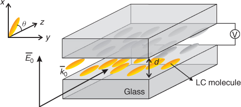
13.3.1 Bias Voltage Switching Time
Many publications on nematicons deal with configurations in which a bias voltage is necessary. Nematic LCs are widely used in display applications, and, obviously, in this type of application, the switching speed of the individual pixels is an important specification for displaying video contents fluently. In essence, the LC cell for the generation of spatial solitons is very similar to a pixel in a display, so one can use the extended literature on liquid crystal displays to find estimates for the switching-on τon and switching-off times τoff of the LC cell. The switching speed in display applications is determined in terms of rise and fall times based on the initial slope of the switching. This initial switching often has an exponential evolution exp( − t/τ). The following estimates can be found for switching a planarly oriented cell without twist [22]:
In Equations 13.20 and 13.21 it is assumed that K11 ≈ K33 = K and V is the applied voltage. The switching time of a cell depends on the material parameters γ and K. But, more importantly, the switching times depend quadratically on the thickness of the LC layer. In displays, the LC layer thickness is typically in the order of 3–5 μm, which results in switching times in the order of tens of milliseconds. In τon, the applied voltage is also present: increasing the applied voltage leads in principle to shorter switching times. However, to achieve certain gray levels, a certain voltage is necessary. Therefore, a common trick in displays is to apply a high voltage for a short time, until the pixel reaches the required gray level, after which the correct voltage is applied. Obviously, the switching-on speeds are not the major problem in displays. The switching-off time is critical as it cannot be reduced by applying a voltage and is governed by surface actions and elastic forces within the liquid crystal.
Equations 13.20 and 13.21 for the switching times provide a good insight in the temporal dynamics of a liquid crystal cell but are not applicable here because the bias voltage for the generation of nematicons is rather small and close to the threshold voltage for switching, for which the earlier equations are not valid. Equations 13.20 and 13.21 apply only to the transition between a high voltage and zero. Figure 13.3 shows results obtained from numerical simulations based on Equation 13.19. Figure 13.3a shows the temporal evolution of θ in the middle of a 75-μm-thick cell when a voltage around the threshold is turned on. Note that no laser-induced director reorientation is considered, so that θ is invariant with respect to y. Figure 13.3b shows the evolution of the rise time versus the applied voltage. The rise time is based on the evolution of the midtilt, that is, the tilt distribution in the middle of the cell (i.e., in the plane x = 0), and is arbitrarily defined as the time for the midtilt to reach 99% of its steady-state value. The switching time is long—on the order of 100 s for 1 V—for two reasons. First, the cell is very thick compared to LC displays; second, the voltage is around threshold. This results in a static electric field of 0.013 V/μm, which gives rise to a very small driving force to reorient the molecules and consequently to a slow process.
Figure 13.3 (a) Evolution of θ in the middle of a 75 μm-thick liquid crystal layer when switching-on the voltage at t = 0 s. (b) Corresponding rise time, that is, the time for the midtilt to reach 99% of its steady-state value versus voltage. Source: Taken from Reference 23.
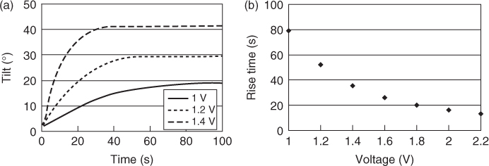
In this one-dimensional case, a scaling of the cell thickness by a factor α results in a scaling of the time by a factor α2, so the results in Figure 13.3 are valid for any cell thickness provided that the time is scaled appropriately.
13.3.2 Soliton Formation Time
Figure 13.4 shows the evolution of the midtilt after turning on the laser beam. The optical beam is a 3-μm-waist TEM00 beam with polarization along the x-axis. The tilt increase in the middle gives rise to a nonhomogeneous increase of the refractive index for light polarized along the x-axis. This self-induced mechanism is responsible for the collimation of the beam through self-focusing.
Figure 13.4 Evolution of the midtilt when turning on a 4.41 mW laser beam at t = 0 s. The voltage across the cell is 1 V. Source: Taken from Reference 23.
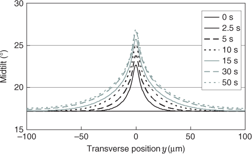
The initial reorientation is relatively fast and takes place on a timescale of a few seconds. Indeed, the reorientation in the middle reaches more than 50% of the final reorientation after 2.5 s. More importantly, it can be seen that the angular profile in the vicinity of the beam center stays almost unchanged after 2.5 s. After this, the reorientation of the molecules further away from the center occurs until an overall steady state is reached with the width of the induced tilt profile much larger than that after a few seconds and, a fortiori, than the solitonlike beam itself. This reorientation occurs on a much larger timescale, and the steady state is reached after about 50 s. This means that the reorientation is initially fast and the nonlocality of the nonlinear effect is small. Then, the nonlocality increases in time until a maximum is achieved. This effect is plausible as only a low energy is required to reorient the liquid crystal in the immediate vicinity of the optical beam. The complete reorientation, whose spatial extent is much wider, requires a much larger energy and, consequently, a longer time.
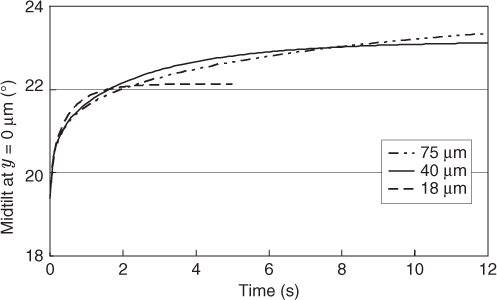
The long time to reach the steady state in thick cells (about 50 s) originates mainly from the large scale of the nonlocal reorientation. Hence, it can be expected that the reorientation time will be much smaller in thinner cells, owing to a less wide molecular reorientation. This is illustrated in Figure 13.5, which shows the evolution of the maximum tilt—that is, the tilt at (x, y) = (0, 0), where the light intensity is maximum. For the 75-μm-thick cell the reorientation takes about 50 s, as illustrated before, but for the thinnest cell (18 μm), the reorientation already reaches its steady-state value after 2 s. For even thinner cells, the time for the overall molecular reorientation to settle is even smaller. However, the initial dynamics are quite similar for thick and thin cells. Indeed, reorientation in the vicinity of the light beam completes in less than 2 s.
Figure 13.5 Simulation of the evolution of the midtilt at y = 0 μm when a 2.25-mW laser beam is turned on at t = 0 s and for different cell thicknesses. Source: Taken from Reference 23.
13.3.3 Experimental Observation of Soliton Formation
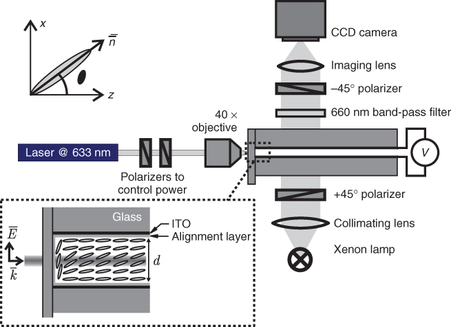
In order to experimentally examine the temporal behavior of soliton formation, the setup in Figure 13.6 was used. A He–Ne laser beam (633 nm) is injected into a liquid crystal cell by use of a 40× microscope objective. The beam propagation in the cell can be observed with the combination of a lens and a CCD camera by collecting the scattered light. Besides light propagation, it is also possible to observe the laser-induced molecular reorientation. This is achieved by using the polarized light from a Xenon lamp. The polarized light traveling through the LC layer undergoes a polarization change depending on the molecular orientation. In this way, the self-induced waveguide can be observed. For such purpose, two crossed polarizers and a band-pass filter (660 nm) are employed, the directions of polarizer and analyzer being ± 45° with respect to the z-axis.
Figure 13.6 Experimental setup and indication of axes. Source: Taken from Reference 23.
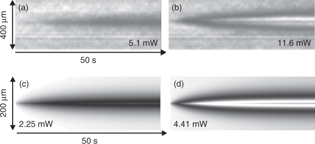
When the optical power is turned on, the beam evolves from a diffracting regime (Figure 13.7a when the molecules are not reoriented yet) to a solitonlike propagation regime (Figure 13.7b). The evolution of the intensity profile of light scattered from the beam after a propagation distance of 1.6 mm is shown in Figure 13.7c. At 0 ms, the width of the beam is large and the intensity is low. After 1 s, the width of the beam has become narrower, the peak intensity higher and the intensity profile reaches a steady state.
Figure 13.7 (a and b) Steady-state light propagation in the cell for a voltage of 1 V: (a) the diffraction regime, that is, for low optical power, and (b) the soliton regime at relatively high optical power (here 2.6 mW). The rectangles show the location where the light intensity is measured. (c) Temporal evolution of the beam intensity for a 2.6-mW optical beam. Light is turned on after the voltage-induced molecular orientation (orientation at rest) reached steady state. Source: Taken from Reference 23.
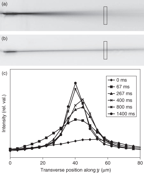
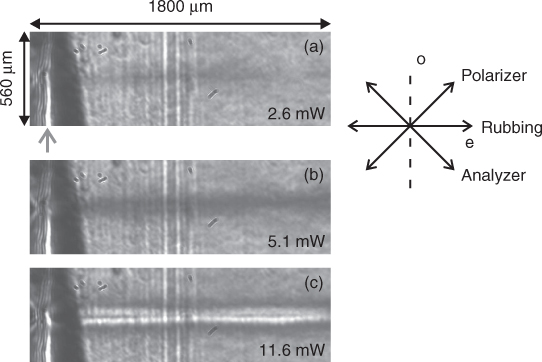
Figure 13.8 shows the polarized transmission image of the cell for different powers of the laser beam. The latter enters from the left side, where the input of the cell is visible. The dark region is caused by glue on top of the interface between the two glass plates. Owing to anisotropy, there is a phase retardation of about 25 × 2π between ordinary and extraordinary polarizations after propagation through the 75-μm-thick cell.1 The laser-induced molecular reorientation reduces the retardation and consequently changes the transmission through the crossed polarizers in the region where the soliton-like beam propagates. In Figure 13.8a, the effect of the reorientation is small, but it increases with increasing optical power (Figure 13.8b and c). With increasing molecular reorientation, the image becomes black, white, and black again as can be seen in Figure 13.8c. This is because the retardation is larger than π. This method of visualizing the self-induced waveguide is clearly not sensitive enough for the small reorientation occurring at 2.6 mW. For this purpose, other approaches are more sensitive, based on interferometry [24] or Raman scattering [25]; to demonstrate the time effects, the described method is useful as the molecular reorientation can be immediately estimated from the transmission profiles.
Figure 13.8 Steady-state transmission of Xenon light through the cell between crossed polarizers, when a laser beam with increasing power from (a) to (c) is launched in the cell. The gray arrow indicates the estimated entrance of the cell. Source: Taken from Reference 23.
The time evolution of the transmission close to the entrance of the 75-μm-thick cell is illustrated in Figure 13.9 for two different optical powers. Owing to the glue at the entrance, it is not possible to define the distance exactly, but it is estimated to be a few hundred micrometers. The two pictures show that the time to completely reorient the liquid crystal is on the order of 50 s. This is in contrast to Figure 13.7c where the formation of the solitonlike beam takes on the order of 1 s. However, it clearly coincides with the findings from numerical simulations. It takes less than a second to reorient the liquid crystal in the vicinity of the beam (although not visible in the transmission experiments) and a few tens of seconds to reorient the liquid crystal further away, related to the large nonlocality of the nonlinearity.
Figure 13.9 Experimental (a and b) and numerical (c and d) evolution of the transmission through the cell after switching on the laser beam. Source: Taken from Reference 23.
As it is clear from the results presented before, the total reorientation of the liquid crystal can be roughly subdivided into two parts. The beam first induces a more or less local reorientation that constitutes a self-induced waveguide. After that, the reorientation relaxes across the whole cell and a slow process of increasing the nonlocal reorientation occurs. The first process occurs in less than 2 s, whereas the second process takes about 50 s to end (for a 50-μm-thick cell). This observation provides a clever way to control the nonlocality of the nonlinearity. When using a continuous beam, after 50 s, the nonlocality is large. However, when chopping the laser beam into pulses of about 2 s and having sufficient time between different pulses, one obtains a local reorientation profile. In this way, the soliton is created, but the director does not get the time to fully relax. By controlling duty cycle of the gated beam, the nonlocality of the nonlinearity can be controlled.
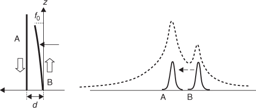
In the work of Henninot et al. [26], this technique was used to investigate the interaction between two counterpropagating solitons as shown in Figure 13.10. One beam (A) is launched from an optical fiber into the LC layer from the top, whereas the other beam (B) is launched from the bottom. Beam A is a CW beam, which means that its self-induced waveguide profile is wide and highly nonlocal. Beam (B) originates from the same laser with equal power, but the beam is chopped with a frequency of 0.25 Hz. Hence, the reorientation profile is more local and this beam can be used as a weak soliton to probe. The experiment revealed that, indeed, the trajectory of the heavy soliton B was not influenced by the presence of the weak soliton A. The lateral deviation from the original trajectory of beam A was used to determine the nonlocal refractive index variation induced by the CW beam B (Chapter 9).
Figure 13.10 Interaction of counterpropagating solitons. A: CW beam, B: pulsed beam. Bold curves represent the solitons, the dashed curve represents the refractive index profile, the white arrows indicate the directions of propagation, and the black arrow indicates the direction of deflection. Source: Taken from Reference 26.
13.3.4 Influence of Flow Effects
In the calculation examples mentioned earlier, the influence of flow in the liquid crystal has been ignored. However, it is known that in certain configurations the flow has an important contribution to the time dependence of the LC switching. In pi cells, for example, the flow can improve the switching [27] by a small factor. Much more dramatic are the effects in vertically aligned liquid crystals with negative Δ ε . Typically, increasing the voltage leads to a faster switching speed. However, voltages higher than a certain threshold lead to a reverse flow phenomenon and a dramatic increase in switching time [28, 29]. This reverse flow is also known as backflow. Owing to backflow, an unwanted twisting of the director occurs and the time to reach the steady state may increase by a factor 100 or higher. Also, in twisted nematic cells, the occurrence of backflow leads to a noticeable difference in switching speed compared to what one would expect in the absence of flow [30–32].
Considering the configuration of the previous sections (Figure 13.4), it is expected that turning on the laser beam will not generate a large amount of flow in the liquid crystal. In order to test the influence of flow on the switching behavior, a 2D modeling program was used that incorporates the flow equations [33, 34]. Figure 13.11 shows the director orientation in terms of the nz component of the director 17 ms after the light is turned on (with 5 mW power). The reorientation of the director is almost a local effect as can be seen from Figure 13.11. The time of 17 ms corresponds more or less to the maximum fluid velocity observed in liquid crystal of about ![]() m/s.
m/s.
Figure 13.11 nz component of the director in a 50-μm-thick cell with 1 V bias voltage, 17 ms after turning on the optical electric field.
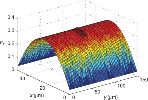
Figure 13.12 shows the different velocity components. The x component of the velocity is the easiest to understand. This speed component shows a strong outward flow above and below the region where the light beam is launched. Because the molecules tilt more, there is a shear flow that repels the molecules to the side of the cell. A simplistic explanation for this effect is that the molecules occupy more space in the x direction when they tilt. An increase in tilt will thus result in a flow outward. The z component of the flow can be explained in a similar manner. Important to note is that vz is antisymmetric with respect to x. The average velocity in the z direction is zero; otherwise, there would be a net flow of material. This is because the pressure of the optical fields is neglected in the simulations. The vy component mainly shows an inward flow from the side, which means that the molecules are mainly flowing away from the region of the light beam along the x-direction and flowing in from the y-direction. The question that now arises is whether these values for the flow affect the switching speed or not.
Figure 13.12 (a–c) Velocity components of the liquid crystal flow, 17 ms after turning on the optical electric field.
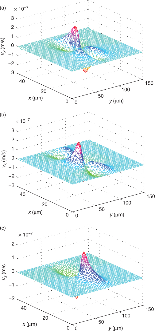
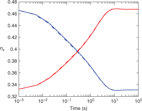
Figure 13.13 shows the evolution of the nx component of the director versus time for the same parameters. When the light beam is turned on, the nx component increases until it reaches steady state after about 10 s. The solid line shows the result when the flow is neglected, and the dashed curve shows the result including flow. It is clear that for these values the influence of flow is negligible. The same conclusion can be drawn when studying the curve for switching off. The flow remains small enough in both cases to have only little influence on the switching behavior.
Figure 13.13 Time evolution of the nx component of the director when switching the beam on and off. For the solid curve, the flow is ignored, while for the dashed curve, the flow is taken into account.
13.4 Conclusions
Liquid crystals exhibit different optical nonlinear effects that can be used to generate spatial optical solitons. It is clear that these nonlinearities have different timescales that affect not only the soliton formation time but also the time it takes to steer or switch soliton beams. In this chapter, we have mainly considered the reorientational nonlinearity as most of the nematicon work has been devoted to this nonlinearity. The formation of the nematicon occurs in less than a few seconds, whereas the actual full reorientation takes a few tens of seconds. During this process, the refractive index change evolves from being nearly local to highly nonlocal, which can be used as a way to control nonlocality.
1 This is because of the large thickness of the cell (75 μm). Nematic LC displays typically have a thickness that is 10–20 times smaller.
1. J. L. Ericksen. Equation of motion for liquid-crystals. Q. J. Mech. Appl. Math., 29: 203–208, 1976.
2. F. M. Leslie. Some constitutive equations for liquid crystals. Arch. Ration. Mech. An., 28(4):265, 1968.
3. H. G. Walton and M. J. Towler. On the response speed of pi-cells. Liq. Cryst., 27(10):1329–1335, 2000.
4. M. Miesowicz. The three coefficients of viscosity of anisotropic liquids. Nature, 158:27, 1946.
5. A. Buka and L. Kramer Eds. Pattern Formation in Liquid Crystals. Springer-Verlag, New York, 1996.
6. W. W. Beens and W. H. Dejeu. Flow-measurements of the viscosity coefficients of 2 nematic liquid-crystalline azoxybenzenes. J. Phys.-Paris, 44(2):129–136, 1983.
7. F. Hennel, J. Janik, J. K. Moscicki, and R. Dabrowski. Improved miesowicz viscometer. Mol. Cryst. Liq. Cryst., 191:401–405, 1990.
8. D. Dunmur, A. Fukuda, and G. Luckhurst Eds. Physical Properties of Liquid Crystals: Nematics. INSPEC, London, 2001.
9. H. Kneppe, F. Schneider, and N. K. Sharma. Rotational viscosity -gamma-1 of nematic liquid-crystals. J. Chem. Phys., 77(6):3203–3208, 1982.
10. P. R. Gerber. Measurement of the rotational viscosity of nematic liquid-crystals. Appl. Phys. A, 26(3):139–142, 1981.
11. H. Kneppe and F. Schneider. Determination of the rotational viscosity coefficient-gamma-1 of nematic liquid-crystals. J. Phys. E Sci. Instrum., 16(6):512–515, 1983.
12. G. Cordoyiannis, D. Apreutesei, G. H. Mehl, C. Glorieux, and J. Thoen. High-resolution calorimetric study of a liquid crystalline organo-siloxane tetrapode with a biaxial nematic phase. Phys. Rev. E, 78(1):011708, 2008.
13. G. Ahlers, D. S. Cannell, L. I. Berge, and S. Sakurai. Thermal-conductivity of the nematic liquid-crystal 4-n-pentyl-4′-cyanobiphenyl. Phys. Rev. E, 49(1):545–553, 1994.
14. K. Y. Kung and H. M. Srivastava. Analytic transient solutions of a cylindrical heat equation with oscillating heat flux. Appl. Math. Comput., 195(2):745–753, 2008.
15. K. T. Chiang, K. Y. Kung, and H. M. Srivastava. Analytic transient solutions of a cylindrical heat equation with a heat source. Appl. Math. Comput., 215(8):2877–2885, 2009.
16. J. Holman. Heat Transfer, McGraw -Hill Series in Mechanical Engineering, 10th edn, 2006.
17. M. Peccianti, A. De Rossi, G. Assanto, A. De Luca, C. Umeton, and I. C. Khoo. Electrically Assisted Self-confinement and Waveguiding in Planar Nematic Liquid Crystal Cells. Appl. Phys. Lett., 77:7–9, 2000.
18. F. Derrien, J. Henninot, M. Warenghem, and G. Abbate. A Thermal (2D+1) Spatial Optical Soliton in a Dye Doped Liquid Crystal. J. Opt. A-Pure Appl. Opt., 2:332–337, 2000.
19. S. V. Serak, N. V. Tabiryan, M. Peccianti, and G. Assanto. Spatial soliton all-optical logic gates. IEEE Photon. Techol. Lett., 18(9–12):1287–1289, 2006.
20. I. B. Burgess, M. Peccianti, G. Assanto, and R. Morandotti. Accessible light bullets via Synergetic Nonlinearities. Phys. Rev. Lett., 102:203903, 2009.
21. I. C. Khoo. Liquid Crystals, Wiley Series in Pure and Applied Optics. 2nd edn, Wiley, Hoboken, New Jersey, 2007.
22. E. Lueder. Liquid Crystal Displays: Addressing Schemes and Electro-Optical Effects, Wiley Series in Display Technology. John Wiley & Sons, Chichester, 2001.
23. J. Beeckman, K. Neyts, X. Hutsebaut, C. Cambournac, and M. Haelterman. Time dependence of soliton formation in planar cells of nematic liquid crystals. IEEE J. Quantum Electron., 41:735–740, 2005.
24. X. Hutsebaut, C. Cambournac, M. Haelterman, J. Beeckman, and K. Neyts. Measurement of the self-induced waveguide of a solitonlike optical beam in a nematic liquid crystal. J. Opt. Soc. Am. B, 22:1424–1431, 2005.
25. M. Warenghem, J. F. Blach, and J. F. Henninot. Measuring and monitoring optically induced thermal or orientational non-locality in nematic liquid crystal. Mol. Cryst. Liq. Cryst., 454:297–314, 2006.
26. J. F. Henninot, J. F. Blach, and M. Warenghem. Experimental study of the nonlocality of spatial optical solitons excited in nematic liquid crystal. J. Opt. A: Pure Appl. Opt., 9:20–25, 2007.
27. P. D. Brimicombe, and E. P. Raynes. The influence of flow on symmetric and asymmetric splay state relaxations. Liq. Cryst., 32(10):1273–1283, 2005.
28. L. Y. Chen and S. H. Chen. Crucial influence of the azimuthal alignment on the dynamics of pure homeotropic liquid crystal cells. Jpn. J. Appl. Phys., 39(4):368–370, 2000.
29. P. J. M. Vanbrabant, N. Dessaud, and J. F. Stromer. Temperature influence on the dynamics of vertically aligned liquid crystal displays. Appl. Phys. Lett., 92(9):091101, 2008.
30. C. Z. van Doorn. Dynamic behavior of twisted nematic liquid-crystal layers in switched fields. J. Appl. Phys., 46(9):3738–3745, 1975.
31. D. W. Berreman. Liquid-crystal twist cell dynamics with backflow. J. Appl. Phys., 46(9):3746–3751, 1975.
32. F. Z. Yang, Y. M. bong, L. Z. Ruan, and J. R. Sambles. Dynamical process of switch-off in a supertwisted nematic cell. J. Appl. Phys., 96(1):310–315, 2004.
33. R. James, E. Willman, F. A. Fernández, and S. E. Day. Finite-element modeling of liquid-crystal hydrodynamics with a variable degree of order. IEEE Trans. Electron Dev., 53:1575–1582, 2006.
34. R. James, E. Willman, F. A. Fernandez, and S. E. Day. Computer modeling of liquid crystal hydrodynamics. IEEE Trans. Magn., 44(6):814–817, 2008.