Chapter 10
Three-Dimensional Plots
Three-dimensional (3-D) plots can be a useful way to present data that consists of more than two variables. MATLAB provides various options for displaying three-dimensional data. They include line and wire, surface, mesh plots, and many others. The plots can also be formatted to have a specific appearance and special effects. Many of the three-dimensional plotting features are described in this chapter. Additional information can be found in the Help Window under Plotting and Data Visualization.
In many ways this chapter is a continuation of Chapter 5, where two-dimensional plots were introduced. The 3-D plots are presented in a separate chapter because not all MATLAB users use them. In addition, new users of MATLAB will probably find it easier to practice 2-D plotting first and learn the material in Chapters 6–9 before attempting 3-D plotting. It is assumed throughout the rest of this chapter that the reader is familiar with 2-D plotting.
10.1 LINE PLOTS
A three-dimensional line plot is a line that is obtained by connecting points in three-dimensional space. A basic 3-D plot ‘is created with the plot3 command, which is very similar to the plot command and has the form:

• The three vectors with the coordinates of the data points must have the same number of elements.
• The line specifiers, properties, and property values are the same as in 2-D plots (see Section 5.1).
For example, if the coordinates x, y, and z are given as a function of the parameter t by

a plot of the points for 0 ≤ t ≤ 6π can be produced by the following script file:
t=0:0.1:6*pi;

x=sqrt(t).*sin(2*t);

y=sqrt(t).*cos(2*t);

z=0.5*t;

plot3(x,y,z,'k','linewidth',1)

grid on

xlabel('x'); ylabel('y'); zlabel('z')
The plot shown in Figure 10-1 is created when the script is executed.

Figure 10-1: A plot of the function ![]() ,
, ![]() , z = 0.5t for 0 ≤ t ≤ 6π.
, z = 0.5t for 0 ≤ t ≤ 6π.
10.2 MESH AND SURFACE PLOTS
Mesh and surface plots are three-dimensional plots used for plotting functions of the form z = f(x, y) where x and y are the independent variables and z is the dependent variable. It means that within a given domain the value of z can be calculated for any combination of x and y. Mesh and surface plots are created in three steps. The first step is to create a grid in the x y plane that covers the domain of the function. The second step is to calculate the value of z at each point of the grid. The third step is to create the plot. The three steps are explained next.
Creating a grid in the x y plane (Cartesian coordinates):
The grid is a set of points in the x y plane in the domain of the function. The density of the grid (number of points used to define the domain) is defined by the user. Figure 10-2 shows a grid in the domain −1 ≤ x ≤ 3 and 1 ≤ y ≤ 4. In this grid the distance between the points is one unit. The points of the grid can be defined by two matrices, X and Y. Matrix X has the x coordinates of all the points, and matrix Y has the y coordinates of all the points:

Figure 10-2: A grid in the x y plane for the domain −1 ≤ x ≤ 3 and 1 ≤ y ≤ 4 with spacing of 1.

The X matrix is made of identical rows since in each row of the grid the points have the same x coordinate. In the same way the Y matrix is made of identical columns since in each column of the grid the y coordinate of the points is the same.
MATLAB has a built-in function, called meshgrid, that can be used for creating the X and Y matrices. The form of the meshgrid function is:

In the vectors x and y the first and last elements are the respective boundaries of the domain. The density of the grid is determined by the number of elements in the vectors. For example, the mesh matrices X and Y that correspond to the grid in Figure 10-2 can be created with the meshgrid command by:

Once the grid matrices exist, they can be used for calculating the value of z at each grid point.
Calculating the value of z at each point of the grid:
The value of z at each point is calculated by using element-by-element calculations in the same way it is used with vectors. When the independent variables x and y are matrices (they must be of the same size), the calculated dependent variable is also a matrix of the same size. The value of z at each address is calculated from the corresponding values of x and y. For example, if z is given by
![]()
the value of z at each point of the grid above is calculated by:
![]()

Once the three matrices have been created, they can be used to plot mesh or surface plots.
Making mesh and surface plots:
A mesh or surface plot is created with the mesh or surf command, which has the form:
![]()
where X and Y are matrices with the coordinates of the grid and Z is a matrix with the value of z at the grid points. The mesh plot is made of lines that connect the points. In the surface plot, areas within the mesh lines are colored.
As an example, the following script file contains a complete program that creates the grid and then makes a mesh (or surface) plot of the function ![]() over the domain −1 ≤ x ≤ 3 and 1 ≤ y ≤ 4.
over the domain −1 ≤ x ≤ 3 and 1 ≤ y ≤ 4.

Note that in the program above the vectors x and y have a much smaller spacing than the spacing earlier in the section. The smaller spacing creates a denser grid. The figures created by the program are:

Additional comments on the mesh command:
• The plots that are created have colors that vary according to the magnitude of z. The variation in color adds to the three-dimensional visualization of the plots. The color can be changed to be a constant either by using the Plot Editor in the Figure Window (select the edit arrow, click on the figure to open the Property Editor Window, then change the color in the Mesh Properties list), or by using the colormap(C) command. In this command C is a three-element vector in which the first, second, and third elements specify the intensity of Red, Green, and Blue (RGB) colors, respectively. Each element can be a number between 0 (minimum intensity) and 1 (maximum intensity). Some typical colors are:
| C = [0 0 0] black | C = [1 0 0] red | C = [0 1 0] green |
| C = [0 0 1] blue | C = [1 1 0] yellow | C = [1 0 1] magenta |
| C = [0.5 0.5 0.5] gray |
• When the mesh command executes, the grid is on by default. The grid can be turned off with the grid off command.
• A box can be drawn around the plot with the box on command.
• The mesh and surf commands can also be used with the form mesh(Z) and surf(Z). In this case the values of Z are plotted as a function of their addresses in the matrix. The row number is on the x axis and the column number is on the y axis.
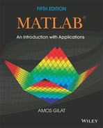
There are several additional plotting commands that are similar to the mesh and surf commands that create plots with different features. Table 10-1 shows a summary of the mesh and surface plotting commands. All the examples in the table are plots of the function ![]() sin (x) cos(0.5y) over the domain −3 ≤ x ≤ 3 and −3 ≤ y ≤ 3.
sin (x) cos(0.5y) over the domain −3 ≤ x ≤ 3 and −3 ≤ y ≤ 3.
Table 10-1: Mesh and surface plots


10.3 PLOTS WITH SPECIAL GRAPHICS
MATLAB has additional functions for creating various types of special three-dimensional plots. A complete list can be found in the Help Window under Plotting and Data Visualization. Several of these 3-D plots are presented in Table 10-2. The examples in the table do not show all the options available with each plot type. More details on each type of plot can be obtained in the Help Window, or by typing help command_name in the Command Window.
Table 10-2: Specialized 3-D plots


Polar coordinates grid in the x y plane:
_A 3-D plot of a function in which the value of z is given in polar coordinates (for example z = rθ) can be done by following these steps:
• Create a grid of values of θ and r with the meshgrid function.
• Calculate the value of z at each point of the grid.
• Convert the polar coordinates grid to a grid in Cartesian coordinates. This can be done with MATLAB’s built-in function pol2cart (see example below).
• Make a 3-D plot using the values of z and the Cartesian coordinates.
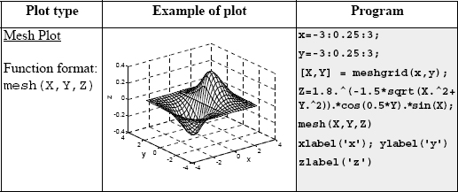
For example, the following script creates a plot of the function z = rθ over the domain 0 ≤ θ ≤ 360° and 0 ≤ r ≤ 2.
The figures created by the program are:

10.4 THE view COMMAND
The view command controls the direction from which the plot is viewed. This is done by specifying a direction in terms of azimuth and elevation angles, as seen in Figure 10-3, or by defining a point in space from which the plot is viewed. To set the viewing angle of the plot, the view command has the form:
![]()
• az is the azimuth, which is an angle (in degrees) in the x y plane measured relative to the negative y axis direction and defined as positive in the counterclockwise direction.
• el is the angle of elevation (in degrees) from the x y plane. A positive value corresponds to opening an angle in the direction of the z axis.
• The default view angles are az = –37.5°, and el = 30°.

Figure 10-3: Azimuth and elevation angles.
As an example, the surface plot from Table 10-1 is plotted again in Figure 10-4, with viewing angles az = 20° and el = 35°.

Figure 10-4: A surface plot of the function ![]() sin (x) cos(0.5y) with viewing angles of az = 20° and el = 35°.
sin (x) cos(0.5y) with viewing angles of az = 20° and el = 35°.
• With the choice of appropriate azimuth and elevation angles, the view command can be used to plot projections of 3-D plots on various planes according to the following table:

An example of a top view is shown next. Figure 10-5 shows the top view of the function that is plotted in Figure 10-1. Examples of projections onto the x z and y z planes are shown next, in Figures 10-6 and 10-7, respectively. The figures show mesh plot projections of the function plotted in Table 10-1.

Figure 10-5: A top view plot of the function ![]() ,
, ![]() , z = 0.5t for 0 ≤ t ≤ 6π.
, z = 0.5t for 0 ≤ t ≤ 6π.

Figure 10-6: Projections onto the x z plane of the function ![]()

Figure 10-7: Projections onto the y-z plane of the function ![]()
• The view command can also set a default view:
view(2) |
sets the default to the top view, which is a projection onto the x-y plane with az = 0°, and el = 90°. |
view(3) |
sets the default to the standard 3-D view with az = –37.5° and el = 30°. |
• The viewing direction can also be set by selecting a point in space from which the plot is viewed. In this case the view command has the form view([x,y,z]), where x, y, and z are the coordinates of the point. The direction is determined by the direction from the specified point to the origin of the coordinate system and is independent of the distance. This means that the view is the same with point [6, 6, 6] as with point [10, 10, 10]. Top view can be set up with [0, 0, 1]. A side view of the x z plane from the negative y direction can be set with [0, −1, 0], and so on.
10.5 EXAMPLES OF MATLAB APPLICATIONS
![]()
Sample Problem 10-1: 3-D projectile trajectory
A projectile is fired with an initial velocity of 250 m/s at an angle of θ = 65° relative to the ground. The projectile is aimed directly north. Because of a strong wind blowing to the west, the projectile also moves in this direction at a constant speed of 30 m/s. Determine and plot the trajectory of the projectile until it hits the ground. For comparison, plot also (in the same figure) the trajectory that the projectile would have had if there was no wind.

Solution
As shown in the figure, the coordinate system is set up such that the x and y axes point in the east and north directions, respectively. Then the motion of the projectile can be analyzed by considering the vertical direction z and the two horizontal components x and y. Since the projectile is fired directly north, the initial velocity ν0 can be resolved into a horizontal y component and a vertical z component:
ν0y = ν0cos(θ) and ν0z = ν0sin(θ)
In addition, due to the wind the projectile has a constant velocity in the negative x direction, νx = −30 m/s
The initial position of the projectile (x0, y0, z0) is at point (3000, 0, 0). In the vertical direction the velocity and position of the projectile are given by:
The time it takes the projectile to reach the highest point (νz = 0) is ![]() . The total flying time is twice this time, ttot = 2thmax. In the horizontal direction the velocity is constant (both in the x and y directions), and the position of the projectile is given by:
. The total flying time is twice this time, ttot = 2thmax. In the horizontal direction the velocity is constant (both in the x and y directions), and the position of the projectile is given by:
x = x0 + νxt and y = y0 + ν0yt
The following MATLAB program written in a script file solves the problem by following the equations above.

The figure generated by the program is shown below.

![]()
Sample Problem 10-2: Electric potential of two point charges
The electric potential V around a charged particle is given by
![]()
where ![]() is the permittivity constant, q is the magnitude of the charge in coulombs, and r is the distance from the particle in meters. The electric field of two or more particles is calculated by using superposition. For example, the electric potential at a point due to two particles is given by
is the permittivity constant, q is the magnitude of the charge in coulombs, and r is the distance from the particle in meters. The electric field of two or more particles is calculated by using superposition. For example, the electric potential at a point due to two particles is given by
![]()
where q1, q2, r1, and r2 are the charges of the particles and the distance from the point to the corresponding particle, respectively.
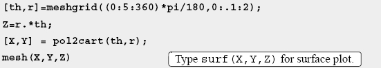
Two particles with a charge of q1 = 2 × 10⁻¹⁰ C and q2 = 3 × 10⁻¹⁰ C are positioned in the x y plane at points (0.25, 0, 0) and (−0.25, 0, 0), respectively, as shown. Calculate and plot the electric potential due to the two particles at points in the x y plane that are located in the domain −0.2 ≤ x ≤ 0.2 and −0.2 ≤ y ≤ 0.2 (the units in the x y plane are meters). Make the plot such that the x y plane is the plane of the points, and the z axis is the magnitude of the electric potential.

Solution
The problem is solved by following these steps:
(a) A grid is created in the x y plane with the domain −0.2 ≤ x ≤ 0.2 and −0.2 ≤ y ≤ 0.2.
(b) The distance from each grid point to each of the charges is calculated.
(c) The electric potential at each point is calculated.
(d) The electric potential is plotted.
The following is a program in a script file that solves the problem.


The plot generated when the program runs is:
![]()
Sample Problem 10-3: Heat conduction in a square plate
Three sides of a rectangular plate (a = 5 m, b = 4 m) are kept at a temperature of 0°C and one side is kept at a temperature T1 = 80°C, as shown in the figure. Determine and plot the temperature distribution T(x, y) in the plate.

Solution
The temperature distribution, T(x, y) in the plate can be determined by solving the two-dimensional heat equation. For the given boundary conditions T(x, y) can be expressed analytically by a Fourier series (Erwin Kreyszig, Advanced Engineering Mathematics, John Wiley and Sons, 1993):

A program in a script file that solves the problem is listed below. The program follows these steps:
(a) Create an X, Y grid in the domain 0 ≤ x ≤ a and 0 ≤ y ≤ b. The length of the plate, a, is divided into 20 segments, and the width of the plate, b, is divided into 16 segments.
(b) Calculate the temperature at each point of the mesh. The calculations are done point by point using a double loop. At each point the temperature is determined by adding k terms of the Fourier series.
(c) Make a surface plot of T.

The program was executed twice, first using five terms (k = 5) in the Fourier series to calculate the temperature at each point, and then with k = 50. The mesh plots created in each execution are shown in the figures below. The temperature should be uniformly 80°C at y = 4 m. Note the effect of the number of terms (k) on the accuracy at y = 4 m.

![]()
10.6 PROBLEMS
1. The position of a moving particle as a function of time is given by:
![]()
Plot the position of the particle for 0 ≤ t ≤ 30.
2. An elliptical staircase that decreases can be modeled by the parametric equations
![]()
where ![]() , a and b are the semimajor and semiminor axes of the ellipse, h is the staircase height, and n is the number of revolutions that the staircase makes. Make a 3-D plot of the staircase with a = 20 m, b = 10 m, h = 18 m, and n = 3. (Create a vector t for the domain 0 to 2πn, and use the
, a and b are the semimajor and semiminor axes of the ellipse, h is the staircase height, and n is the number of revolutions that the staircase makes. Make a 3-D plot of the staircase with a = 20 m, b = 10 m, h = 18 m, and n = 3. (Create a vector t for the domain 0 to 2πn, and use the plot3 command.)

3. The ladder of a fire truck can be elevated (increase of angle ![]() ) rotated about the z axis (increase of angle θ), and extended (increase of r). Initially the ladder rests on the truck (
) rotated about the z axis (increase of angle θ), and extended (increase of r). Initially the ladder rests on the truck (![]() = 0, θ = 0, and r = 8m). Then the ladder is moved to a new position by raising the ladder at a rate of 5 deg/s, rotating at a rate of 8 deg/s, and extending the ladder at a rate of 0.6 m/s. Determine and plot the position of the tip of the ladder for 10 seconds.
= 0, θ = 0, and r = 8m). Then the ladder is moved to a new position by raising the ladder at a rate of 5 deg/s, rotating at a rate of 8 deg/s, and extending the ladder at a rate of 0.6 m/s. Determine and plot the position of the tip of the ladder for 10 seconds.

4. Make a 3-D surface plot of the function ![]() in the domain −3 ≤ x ≤ 3 and −3 ≤ y ≤ 3.
in the domain −3 ≤ x ≤ 3 and −3 ≤ y ≤ 3.
5. Make a 3-D surface plot of the function z = 0.5x2 + 0.5y2 in the domain −2 ≤ x ≤ 2 and −2 ≤ y ≤ 2.
6. Make a 3-D mesh plot of the function ![]() , where
, where ![]() in the domain −5 ≤ x ≤ 5 and −5 ≤ y ≤ 5.
in the domain −5 ≤ x ≤ 5 and −5 ≤ y ≤ 5.
7. Make a 3-D surface plot of the function ![]() in the domain −2π ≤ x ≤ 2π and −π ≤ y ≤ π.
in the domain −2π ≤ x ≤ 2π and −π ≤ y ≤ π.
8. Make a plot of the ice cream cone shown in the figure. The cone is 8 in. tall with a 4 in. diameter base. The ice cream at the top is a 4 in. diameter hemisphere.
A parametric equation for the cone is:
x = r cosθ, y = r sinθ, z = 4r
with 0 ≤ θ ≤ 2π and 0 ≤ r ≤ 2
A parametric equation for a sphere is:
![]()

9. The van der Waals equation gives a relationship between the pressure p (atm), volume V, (L), and temperature T(K) for a real gas:
![]()
where n is the number of moles, R = 0.08206(L atm)/(mol K) is the gas constant, and a (L2 atm/mol2), and b (L/mol) are material constants.
Consider 1.5 moles of nitrogen (a = 1.39 L2 atm/mol2, b = 0.03913 L/mol). Make a 3-D plot that shows the variation of pressure (dependent variable, z axis) with volume (independent variable, x axis) and temperature (independent variable, y axis). The domains for the volume and temperature are 0.3 ≤ V ≤ 1.2 L and 273 ≤ T ≤ 473 K.
10. Molecules of a gas in a container are moving around at different speeds. Maxwell’s speed distribution law gives the probability distribution P(ν) as a function of temperature and speed:
![]()
where M is the molar mass of the gas in kg/mol, R = 8.31 J/(mol K), is the gas constant, T is the temperature in kelvins, and ν is the molecule’s speed in m/s.
Make a 3-D plot of P(ν) as a function of ν and T for 0 ≤ ν ≤ 1000 m/s and 70 ≤ T ≤ 320 K for oxygen (molar mass 0.032 kg/mol).
11. Plank’s distribution law gives the blackbody emissive power (amount of radiation energy emitted) as a function of temperature and wave length:
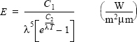

where C1 = 3.742 × 10⁸ Wμm4/m2, C2 = 1.439 × 10⁴ μmK, T is the temperature in degrees K, and λ is the wave length in μm. Make a 3-D plot (shown in the figure) of E as a function of λ (0.1 ≤ λ ≤ 10 μm) and T for 100 ≤ T ≤ 2000 K. Use a logarithmic scale for λ. This can be done with the command: set(gca,‘xscale’,‘log’).
12. The flow Q (m3/s) in a rectangular channel is given by the Manning’s equation:
![]()
where d is the depth of water (m), w is the width of the channel (m), S is the slope of the channel (m/m), n is the roughness coefficient of the channel walls, and k is a conversion constant (equal to 1 when the units above are used). Make a 3-D plot of Q (z axis) as a function of w (x axis) for 0 ≤ w ≤ 8 m, and a function of d (y-axis) for 0 ≤ d ≤ 4 m. Assume n = 0.05 and S = 0.001 m/m.
13. An RLC circuit with an alternating voltage source is shown. The source voltage νs is given by νs = νm sin(ωdt), where ωd = 2πfd, in which fd is the driving frequency. The amplitude of the current, I, in this circuit is given by:
![]()

where R and C are the resistance of the resistor and capacitance of the capacitor, respectively. For the circuit in the figure C = 15 × 10−6 F, L = 240 × 10−3 H, and νm = 24 V.
a) Make a 3-D plot of I (z axis) as a function of ωd (x axis) for 60 ≤ f ≤ 110 Hz, and as a function of R (y axis) for 10 ≤ R ≤ 40 Ω
b) Make a plot that is a projection on the x z plane. Estimate from this plot the natural frequency of the circuit (the frequency at which I is maximum). Compare the estimate with the calculated value of ![]() .
.
14. A defect in a crystal lattice where a row of atoms is missing is called an edge dislocation. The stress field around an edge dislocation is given by:


where G is the shear modulus, b is the Burgers vector, and ν is Poisson’s ratio. Plot the stress components (each in a separate figure) due to an edge dislocation in aluminum, for which G = 27.7 × 10⁹ Pa, b = 0.286 × 10⁻⁹ m, and ν = 0.334. Plot the stresses in the domain −5 × 10⁻⁹ ≤ x ≤ 5 × 10⁻⁹ m and −5 × 10⁻⁹ ≤ y ≤ −1 × 10⁻⁹ m. Plot the coordinates x and y in the horizontal plane, and the stresses in the vertical direction.
15. The current I flowing through a semiconductor diode is given by
![]()

where Is = 10−12 A is the saturation current, q = 1.6 × 10⁻¹⁹ C is the elementary charge value, k = 1.38 × 10⁻²³ J/K is Boltzmann’s constant, νD is the voltage drop across the diode, and T is the temperature in kelvins. Make a 3-D plot of I (z axis) versus νD (x axis) for 0 ≤ νD ≤ 0.4, and versus T (y axis) for 290 ≤ T ≤ 320K.
16. The equation for the streamlines for uniform flow over a cylinder is
![]()
where ψ is the stream function. For example, if ψ = 0, then y = 0. Since the equation is satisfied for all x, the x axis is the zero (ψ = 0) streamline. Observe that the collection of points where x2 + y2 = 1 is also a streamline. Thus, the stream function above is for a cylinder of radius 1. Make a 2-D contour plot of the streamlines around a cylinder with 1 in. radius. Set up the domain for x and y to range between −3 and 3. Use 100 for the number of contour levels. Add to the figure a plot of a circle with a radius of 1. Note that MATLAB also plots streamlines inside the cylinder. This is a mathematical artifact.
17. The deflection w of a clamped circular membrane of radius rd subjected to pressure P is given by (small deformation theory)
![]()
where r is the radial coordinate, and ![]() , where E, t, and υ are the elastic modulus, thickness, and Poisson’s ratio of the membrane, respectively. Consider a membrane with P = 15 psi, rd = 15 in., E = 18 × 106 psi, t = 0.08 in., and υ = 0.3. Make a surface plot of the membrane.
, where E, t, and υ are the elastic modulus, thickness, and Poisson’s ratio of the membrane, respectively. Consider a membrane with P = 15 psi, rd = 15 in., E = 18 × 106 psi, t = 0.08 in., and υ = 0.3. Make a surface plot of the membrane.
18. The Verhulst model, given in the following equation, describes the growth of a population that is limited by various factors such as overcrowding and lack of resources:

where N(t) is the number of individuals in the population, N0 is the initial population size, N∞ is the maximum population size possible due to the various limiting factors, and r is a rate constant. Make a surface plot of N(t) versus t and N∞ assuming r = 0.1 s−1, and N0 = 10. Let t vary between 0 and 100 and N∞ between 100 and 1,000.
19. The geometry of a ship hull (Wigley hull) can be modeled by the equation
![]()

where x, y, and z are the length, width, and height, respectively. Use MATLAB to make a 3-D figure of the hull as shown. Use B = 1.2, L = 4, T = 0.5, −2 ≤ x ≤ 2, and −0.5, ≤ z ≤ 0.
20. The stresses fields near a crack tip of a linear elastic isotropic material for mode I loading are given by:


For ![]() plot the stresses (each in a separate figure) in the domain 0 ≤ θ ≤ 90° and 0.02 ≤ r ≤ 0.2 in. Plot the coordinates x and y in the horizontal plane, and the stresses in the vertical direction.
plot the stresses (each in a separate figure) in the domain 0 ≤ θ ≤ 90° and 0.02 ≤ r ≤ 0.2 in. Plot the coordinates x and y in the horizontal plane, and the stresses in the vertical direction.
21. A ball thrown up falls back to the floor and bounces many times. For a ball thrown up in the direction shown in the figure, the position of the ball as a function of time is given by:
![]()

The velocities in the x and y directions are constants throughout the motion and are given by νx = ν0 sin(θ) cos (α) and νy = ν0 sin(θ) sin (α). In the vertical z direction the initial velocity is νz = ν0 cos(θ), and when the ball impacts the floor its rebound velocity is 0.8 of the vertical velocity at the start of the previous bounce. The time between bounces is given by tb = (2νz)/g, where νz is the vertical component of the velocity at the start of the bounce. Make a 3-D plot (shown in the figure) that shows the trajectory of the ball during the first five bounces. Take ν0 = 20 m/s, θ = 30°, α = 25°, and g = 9.81 m/s2.
