
11
Probabilistic Potential Theory
11.1 Random Walks and the Diffusion Equation
Consider a grid with nodes (i, j) spaced one unit apart in both axes. These nodes, at this point, have nothing to do with electrostatics –– there are no voltages, charges, or fields present. Instead, there is a particle undergoing a random walk. Brownian motion,1 for example, is a random walk of particles. Random walks have various defining characteristics; the random walk discussed here is defined as follows:
- There is a particle sitting at one of the nodes. At time (m − 1) the probability of the particle being at node (i, j) is Pm−1(i, j).
- Every second the particle will quickly jump to an adjacent node. Adjacent means to the left (−x), right (+x), up (+y) or down (−y). Diagonal jumps and multinode jumps are not allowed.
- All of the jumps have equal probability; that is, the probability of any given jump is
 .
.
Four examples of such a walk, reminiscent of a drunkard wandering through a parking lot, are shown in Figure 11.1. In each of these examples the particle started at (0,0).
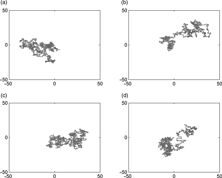
FIGURE 11.1 Four fixed-step two-dimensional random walks.
At a given time, a particle can arrive at node (i, j) only if it started from one of the (four) adjacent nodes. The probability of a particle arriving at node (i, j) is therefore
If the particle had been at node (i, j) at time m − 1, since it had to jump to somewhere, there is a 100% probability (i.e., it is certain) that it is no longer at node (i, j) at time m. The net change in the probability of the particle being in cell (i,j) at time m as compared to the probability that it was at node (i,j) at time m − 1 is therefore
If we look over many time intervals and require that the net change be zero, that is, look for the steady-state situation, equation (11.2) is set equal to zero, and we have
This equation should look familiar.
As an aside, a formal derivation, taking the proper limits and including proper physical constants, leads to the diffusion equation.2 In rectangular coordinates and two dimensions, this is
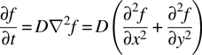
In the steady state the left-hand side (LHS) of this equation is zero, leading to
This is identically Laplace's equation, and then equation (11.3) is the finite difference numerical approximation to Laplace's equation that we've been dealing with all along.
One last point — the diffusion equation looks a lot like the wave equation:

The wave equation and the diffusion equation describe different physical phenomena and are identical only when derivatives with respect to time are zero.
The equivalence of the steady-state wave and diffusion equations leads us to a solution technique for electrostatics problems, sometimes called probabilistic potential theory 3 (PPT), which is distinctly different from anything we've looked at so far. This technique relies on a random-walk game with a set of rules for play and scoring, while physical terms such as electric field, charge, or energy never appear.
11.2 Voltage at a Point from Random Walks
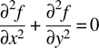
Consider the two-dimensional (2d) cross section shown in Figure 11.2. The figure shows an inner rectangular box asymmetrically located inside an outer rectangular box. Not shown is a 1 × 1 grid of points that these boxes sit on. The outer box is set at 0 V; the inner box is set at 1 V. The point (0,12) — arbitrarily chosen — is the point at which we want to learn the voltage. There are several approaches to treating this as a random-walk probabilistic problem rather than an electrostatics problem.
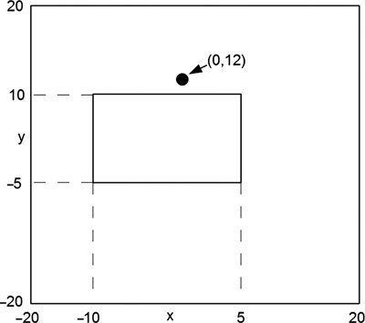
FIGURE 11.2 Two-dimensional structure example for PPT analysis.
The first approach is a random-walk game. Assume that a “random walker” is placed at point (0,12). He then takes his random walk, as described above and exemplified in Figure 11.1. When he hits either the inner or the outer box (boundary condition electrode), his walk is over; he is extracted from the game and the identity of the box that he hit is recorded.
This procedure is repeated a number of times (how many times is necessary will be discussed below). If n 1 is the number of extractions at the inner box and n 0 the number of extractions at the outer box, then the probability of starting at point (0,12), taking a random walk as described above and being extracted at the inner box, is
Since both the random walk and the finite-difference Laplace equations are the same, this probability is identically the voltage at point (0,12) when the inner and outer boxes are electrodes at 1 and 0 volts, respectively. Equation (11.7) is an approximation to the probability. We expect this approximation to improve as the number of random walkers (n 0 + n 1) take their walk, but some discussion of “improve” is necessary — this equation does not converge to the correct answer in the same manner as a Gauss–Seidel relaxation converges to the correct answer. Also, of course, this solution technique can only be as good (or as bad) as the resolution of the grid. In this respect it is identical to the finite difference solutions discussed in previous chapters.
When (n0 + n1) random walkers take their walks, the probability of getting a certain number of these to be extracted at the inner conductor, when the probability of any one of them being extracted at the inner conductor is n1, is calculated using the binomial probability formula. The binomial formula is standard probability-and-statistics text material.4,5 Only relevant results and their interpretation will be presented here.
For a large number of samples (in statistics jargon, the results of each random walk discussed above is a sample), the binomial probability distribution is indistinguishable from the normal, or Gaussian, distribution (a bell curve).
Relating the two distributions, for n = (n 0 + n 1), the number of samples and p the probability for each of the samples, the mean of the normal distribution is
and the standard deviation is
Figure 11.3 shows a normal distribution. The curve is symmetric about the mean μ, which in this example is 5. The standard deviation of this curve σ is 1. The two vertical lines are at x = μ + 1.96σ and μ – 1.96σ (1.96 is often simply rounded to 2 in this situation). The area under the curve between the two lines occupies 95% of the total area under the curve. This is interpreted to mean that, for a very large number of samples, 95% of the results will fall between these two lines. This is referred to as the 95% confidence interval. Had we chosen three sigma 3σ above and below the mean, we would find that ~99% of the area under the curve and this wider region would be our 99% confidence interval.
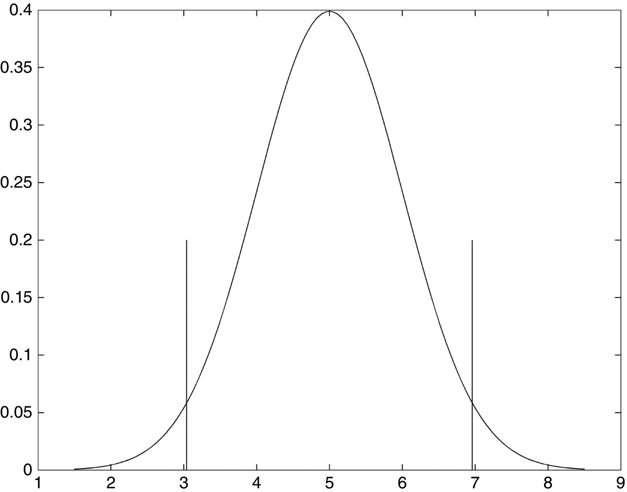
FIGURE 11.3 Graph of a normal distribution; μ = 5, σ = 1.
Relating all of this back to our example, if the probability of n 1 extractions at the center conductors out of n total starts is
we expect the distribution of our n results to resemble a normal distribution (for n sufficiently large) that obeys equations (11.8) and (11.9).
Suppose that we want a 95% confidence interval that is 5% (of the mean) wide. Then
Using equations (11.8) and (11.9) and solving for n, we find that

where n is the number of random walk starts we need to give us a 5% wide confidence interval about p, where p is the voltage at the starting point — our desired result. At this point we seem to be chasing our collective tail. We want to know the minimum n that will let us find p with some measure of confidence, but we first need to know p in order to find n.
This dilemma is resolved by an iterative procedure, as will be shown in MATLAB program ppt1.m below. We take (what we hope to be) a representative number of random-walk starts and then calculate n using equation (11.12). If our number of starts is less than n, we repeat the process. Eventually the predicted value of n becomes relatively constant and then at some point we have made n starts.
Figure 11.4 shows the results of 10 runs of the program.
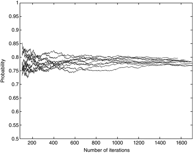
FIGURE 11.4 Repeated runs of program ppt1.m showing convergence of results.
The figure shows that in all of these runs the probability approaches approximately 0.78, but no two runs are identical. If we were to repeat this procedure hundreds of times, we'd find that approximately 95% of the probabilities were within 5% of the average of these probabilities, and if we repeated the procedure thousands of times to accumulate enough data to plot a smooth curve, we'd find a normal distribution of probabilities with the correct characteristics.
Here is MATLAB program ppt1.m — example of a 2d PPT calculation:
% ppt1 Simple 2d random walk ppt example

tic     % turn on timer function

% outer box is a square at x = + - max,y = + - max
max = 20;

% inner box is a rectangle, dimensions as shown
x1 = -10; x2 = 5; y1 = -5; y2 = 10;

% set atarting point
x_start = 0; y_start = 12;

% Intialize counters
nr_iters = 500;       % starting max number of iterations
nr_ones = 0;           % number of hits to 1 volt electrode
iter = 0;           % random walker counter
nr_sigs = 1.96;       % number of sigmas for confidence factor
conf_width = .025;      % half-width fraction about mean for nr_sigs confidence
iter_plot = []; p_plot = []; % arrays to store p(n) for a plot

while iter < nr_iters   % Random walks

 iter = iter + 1 ;
 hit_boundary = 0;       % wandering point flag
 x = x_start; y = y_start;    % starting point
 while hit_boundary < = 0
  p = rand;
  if p < 1/4
   x = x -1;
  elseif p < 2/4
   x = x + 1;
  elseif p < 3/4
   y = y - 1;
  else
   y = y + 1;
  end

  if abs(x) == max | abs(y) == max
   hit_boundary = 1 ; % outer box
  end

  if x > = x1 & x < = x2 & y > = y1 & y < = y2
   hit_boundary = 2;   % inner brick top or bottom
  end
end

if hit_boundary == 2   % Inner box hit counter
 nr_ones = nr_ones + 1;
end

if iter > 100       % Error predictor
  p = nr_ones/iter;   % working intermediate probability
  nr_iters = ceil((nr_sigs/conf_width)^2*(1 - p)/p);
  iter_plot = [iter_plot, iter];
  p_plot = [p_plot, p];
 end

end

volts = nr_ones/nr_iters;

fprintf ('Number of iterations = %d
', nr_iters)
fprintf ('Voltage at starting point = %6.3f
', volts)
toc

plot(iter_plot, p_plot, 'k')
axis ([80, nr_iters + 20, .5, 1.]);
xlabel ('Number of Iterations')
ylabel ('Probability')
hold on
An interesting attribute of this calculation is that the number of iterations required for a given confidence level of the result is a function of that result. If p (which in the example above is the voltage at the random walk’s starting point) is close to one, the scaling factor (1 – p)/p in equation (11.12) is much less than one. On the other hand, if p is very small (e.g., for a point near the 0 V outer box), then this scaling factor begins to exceed 1 significantly. In other words, many more random walks are needed to calculate V at a point if its voltage is close to zero than to one.
This calculation property occurs because of the way in which the acceptable confidence level was specified in equation (11.11). A fixed percentage change of a small number is much smaller than the same fixed percentage change of a large number. Asking for a 5% window centered on (say) 0.01 V is asking much more than asking for a 5% window centered on (say) 0.99 V. From a conventional statistics perspective, we are saying that it's much easier, in terms of the number of data points needed, to be confident about the statistics of a fairly certain event than it is to be confident about the statistics of a fairly rare event.
Interchanging the electrode voltage settings doesn't reduce this problem. Suppose that we set the outer box in Figure 11.1 to 1 V and the inner box to 0 V, and we find the voltage at some point near the outer box to be 0.85 V. Then all we have to do to get the voltage at that point in the original configuration is to subtract this number from 1: specifically 1.00 − 0.85 = 0.15 V. The problem is that if we had found the 0.85 V with a 95% confidence interval of (say) 0.02 V above and below 0.85, then we would know the 0.15 V answer to 0.02 V only above and below 0.15. This latter confidence interval is, on a percentage basis, much higher than the confidence interval at 0.85 V.
For high probability points we have another problem. The calculated necessary number of starting walkers gets so low that we have to make sure that we are getting meaningful numerical results. For example, if p = 0.98, then, on average, only 2% of the starting walkers will be extracted at the outer boundary. Starting 50 walkers at this point will produce numerical nonsense. We need to set a minimum number of iterations (about 1000 in this example) to ensure reasonable statistics.
Variations of the relaxation equation due to dielectric interfaces and/or unequal grid steps can be translated directly into probabilistic interpretations and the random-walk probabilities adjusted accordingly. For example, using the results in Chapter 9, at a dielectric interface along the y axis, we get

and the probability of a step in the -y direction is
and so on.
Uneven node separations, as treated in Chapter 9, are handled the same way. Similarly, a three-dimensional (3d) finite difference grid becomes a 3d random walk. For a simple uniform grid, the probability of any one step is ![]() .
.
If the voltage (Figure 11.1) on the inner and outer boxes had been, say, 870 and 0 V, respectively, then the random-walk problem would be the same as above, but when p is found, it must be scaled by a factor of 870. Combinations of multiple electrodes at arbitrary different voltages are handled in a similar manner.
Figure 11.5 shows a three-electrode structure with the electrodes set at voltages as indicated in the figure:
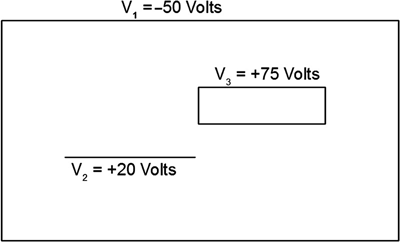
FIGURE 11.5 Structure with several electrodes and electrode voltages.
The procedure for setting up the scaling and offsets is as follows:
- Offset all the voltages so that the most negative of them is zero. In this case, subtract −50 from all the values:

- Scale all the voltages so that the highest voltage is 1.0. In this case, divide all the voltages by 125.

- Run the random-walk program with the following rules:
- The random walk starts at the desired gridpoint, as previously
- The walker is extracted on reaching any of the electrodes
-
The number of extractions at each electrode is recorded (n 1 = number of extractions at electrode number 1, etc.). Then calculate the probability using the weighted sum
(11.15)
-
Now suppose that we find that p = 0.5. First, reverse the scaling: 0.5(125) = 62.5. Then reverse the offset:

The random-walk procedure is an interesting but at this point unsatisfying way to solve the finite difference Laplace equation. Two criticisms are that substantial effort has gone into finding the voltage at only one point rather than over the entire grid, and that the accuracy is a statistical bet — a 95% confidence interval doesn't really guarantee anything. For that matter, if this procedure were used over many points on a grid to determine the voltages at all these points, some of the voltages (about 5% of them) will definitely fall outside the confidence interval.
The procedure in Section 11.3 will be more satisfying in this latter respect because the diffusion equation will be solved without resorting to random walks, or for that matter to random numbers at all.
11.3 Diffusion
The random-walk solution technique as used above repeatedly started one random walker at the point of interest, stayed with him until he was extracted at an electrode, and then started another random walker. The same calculation could have been accomplished by starting a large number of random walkers simultaneously and tracking them all as they meandered about the grid. This is actually our intuitive picture of diffusion. If you put a small drop of cream into a cup of coffee, you can watch as molecules of cream take their random walks and spread out, or diffuse, until the cream is uniformly distributed in the coffee. If the walls of the coffee cup were chemical filters of some sort that absorbed the cream molecules rather than reflecting them back into the coffee, this coffee cup would be a good chemical analogy of our problem solving technique.
If the number of random walkers is very large, then we don't need a random-number generator to tell us which way each of them goes. We don't really care which walker goes which way; just knowing that (in two dimensions) 25% of the walkers at every gridpoint will go one step in each direction on the grid is all the information we need.
We can start with some large number of walkers at the starting point, but this becomes awkward when we get to a point that has, say, three walkers — how do we assign their position at the next step? Instead, start with 1.0 walker and send 0.25 each way. Physically we're following the same procedure; we're just sidestepping some numerical nonsense. The discussion below will still refer to walker, with the understanding that these are all numbers less than 1.0 rather than integers representing individuals.
The diffusion program proceeds in the following manner:
- Put 1.0 walkers at the starting point.
- At each iteration, at every point on the grid transfer
 of the walkers from that gridpoint to each of the (4) adjacent gridpoints. Extract walkers at the electrodes and keep score as in the random walker program.
 - When there is only some predetermined number of walkers left on grid, terminate the process and calculate the final probability. If we set the termination number, for example, for 10−6 walkers left on the grid, then we have a fixed voltage tolerance. On the other hand, if we update the (no longer) predetermined number to a fraction of the probability as we learn it, then we have a tolerance that is a percentage about the final probability.
MATLAB program ppt2.m—a repeat of the—previous problems, solved using diffusion performs this calculation:
% ppt2 repeat of ppt1 example, solved by diffusion

% All dimensions are re-referenced for Matlab indices
% i.e. max has been added to every x & y value so that
% array indices always start at 1

max = 20; % These are the definitions from ppt1
% inner box is a rectangle, dimensions as shown

x1 = 11; x2 = 26; y1 = 16; y2 = 31;

% set starting point
x_start = 21; y_start = 33;

s = zeros(2*max + 1); % array showing current status
s(x_start, y_start) = 1; % initialization

done = 0.;   % extraction monitor
prob = 0.;   % center conductor hit totaller

% Numbers will be moved from s to s2 so as to keep them
% separate, then after every point has been diffused, s2
% will be transferred back to s for the next iteration

x_plot = []; prob_plot = []; % Arrays for observing convergence

tic
while done < .999 % This sets .001 as the "done" level

 s2 = zeros(2*max + 1);   % clear s2
 for i = 2:2*max       % diffuse
  for j = 2:2*max
   s2(i-1,j ) = s2(i-1,j) + s(i,j)/4.;
   s2(i + 1,j) = s2(i + 1,j) + s(i,j)/4.;
   s2(i,j-1) = s2(i,j-1) + s(i,j)/4.;
   s2(i,j + 1) = s2(i,j + 1) + s(i,j)/4.;
  end
 end

 s2(1,:) = 0 ;   % extract at outer box
 s2(2*max + 1,:) = 0;
 s2(:,1) = 0 ;
 s2(:,2*max + 1) = 0;

 for i = x1:x2   % score then extract at inner box
  for j = y1:y2
   prob = prob + s2(i,j);
   s2(i,j) = 0;
  end
end

 done = 1 - sum(sum(s2));   % monitor extraction
 s = s2;             % reestablish s

 prob_plot = [prob_plot,prob];

end
toc

fprintf ('Final probability = %6.3f
', prob)

plot(prob_plot, 'k')
axis ([0, length(prob_plot) + 20, 0., 1.])
xlabel('Number of Iterations')
ylabel('Probability')

save s.txt s -ascii
Using a final remaining number of 0.001 as the termination condition, the program produces a voltage at the starting point of 0.782. Figure 11.6 shows the convergence of the probability with iterations.
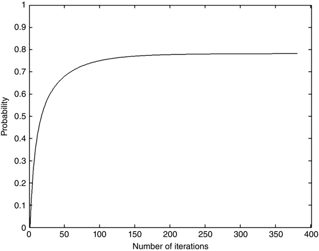
FIGURE 11.6
Convergence of the probability as calculated by ppt2.m.
Comparing Figures 11.6 and 11.4, it is clear how eliminating the random-number generator greatly improved the smoothness of convergence. Also, there is no variation — this program will produce the same results every time it is run.
11.4 Variable-Step-Size Random Walks
The two previous sections showed two techniques for performing a finite difference calculation by taking advantage of the equivalence between the numerical Laplace equation and the steadystate numerical diffusion equation. These calculations, although interesting, brought nothing to the party in terms of practical problem solution. Possibly, if information about the voltage is needed at only very few points, these solution techniques are more efficient than simply solving the entire set of equations.
Another approach to a random-walk solution is to eliminate the grid entirely.
Figure 11.7 shows the same example as shown in Figure 11.2. It has been reconfigured a bit for clarity, so it doesn't look exactly the same as Figure 11.2.
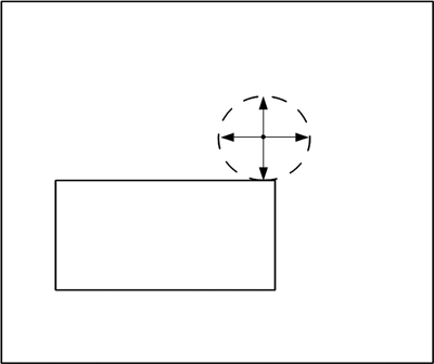
FIGURE 11.7 Two-dimensional potential problem with no grid.
In Figure 11.7, a circle has been drawn about the starting point. The radius of the circle is chosen such that it is tangent to the boundary line (electrode) closest to the starting point. A temporary square grid is established as shown by the arrows, with the starting point and the tangent point of the circle establishing the gridpoint separations.
The random walker now takes a step from the starting point to one of the four gridpoints. She has a ![]() probability of landing on an electrode and being extracted.
probability of landing on an electrode and being extracted.
Figure 11.8a shows one of the other possibilities, the next circle, and the next temporary grid. In this case the gridpoints do not lie along the x and y axes — and there is no need for them to be along these axes. Figure 11.8b shows a possible third circle and set of gridpoints. There is always a 25% probability that the walker will be extracted, this time at the outer electrode.
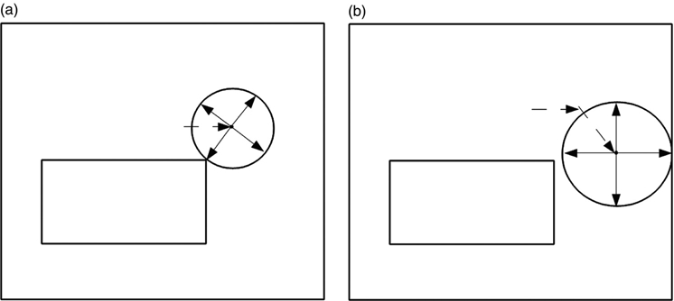
FIGURE 11.8 Further possible random steps, following Figure 11.7.
After three steps, the probability of having been extracted is greater than 50%:
This probability climbs rapidly with the number of steps taken. After six steps, it is
The average walk doesn't take long. Computationally, computer time needed for these shorter walks is offset by the complexity of finding the closest wall and calculating the temporary grid. If there is a dielectric interface, then this interface should be considered a wall insofar as calculating a temporary grid, and we can use equation (11.13) directly to calculate the probabilities of steps. Consider the following programs:
- Program
ppt3.m— repeat of previous example using nongridded PPT:% ppt3 ppt1 example by non-gridded solution tic % turn on timer function max = 20; % This is the definition from ppt1 % inner box is a rectangle, dimensions as shown x1 = -10; x2 = 5; y1 = -5; y2 = 10; % set starting point x_start = 0; y_start = 12; % The first task is to categorize all lines (electrode edges) % The array al has a row for each line. Columns are: % 1. Line type. 1 = horizontal, 2 = vertical % 2. Location. y value for horizontal, x value for vertical % 3,4. Start & stop. x1, x2 for horizontal, y1, y2 for vertical % 5. Voltage al = zeros(8,5); % Block out the al (all_lines) array % This is brute force - a better program would have a subroutine doing this % or it could be stored information in a data file al(1,1) = 1; % top outer box horizontal line al(1,2) = max; al(1,3) = -max; al(1,4) = max; al(1,5) = 0.; al(2,1) = 1; % bottom outer box horizontal line al(2,2) = -max; al(2,3) = -max; al(2,4) = max; al(2,5) = 0.; al(3,1) = 2; % left outer box vertical line al(3,2) = -max; al(3,3) = -max; al(3,4) = max; al(3,5) = 0; al(4,1) = 2; % right outer box vertical line al(4,2) = max; al(4,3) = -max; al(4,4) = max; al(4,5) = 0; al(5,1) = 1; % top inner box horizontal line al(5,2) = y2; al(5,3) = x1; al(5,4) = x2; al(5,5) = 1.; al(6,1) = 1; % bottom inner box horizontal line al(6,2) = y1; al(6,3) = x1; al(6,4) = x2; al(6,5) = 1.; al(7,1) = 2; % left inner box vertical line al(7,2) = x1; al(7,3) = y1; al(7,4) = y2; al(7,5) = 1; al(8,1) = 2; % right inner box vertical line al(8,2) = x2; al(8,3) = y1; al(8,4) = y2; al(8,5) = 1; nr_walls = length(al); % Intialize counters nr_iters = 500; % starting max number of iterations nr_ones = 0; % number of hits to 1 volt electrode iter = 0; % random walker counter nr_sigs = 1.96; % number of sigmas for confidence factor conf_width = .025; % half-width fraction about mean for nr_sigs confidence iter_plot = []; p_plot = []; % arrays to store p(n) for a plot nr_steps = []; % monitor number of steps per walk % Random walks while iter < nr_iters iter = iter + 1 ; hit_boundary = 0; % wandering point flag x = x_start; y = y_start; % start at starting point steps = 0; % count nr steps per walk - not necessary while hit_boundary < = 0 % this is the particle wandering loop steps = steps + 1; % Find the closest wall dists = []; for i = 1:nr_walls if al(i,1) == 1 dist = hor_line_dist(al(i,2:4),[x,y]); dists = [dists;dist]; else dist = vert_line_dist(al(i,2:4),[x,y]); dists = [dists;dist]; end end [min_dist, index] = min(dists(:,1)); % min dist and col nr p1 = dists(index,2:3); % This is the point on a boundary rad = norm([p1(1) - x,p1(2) - y]); % size of step theta = atan2(p1(2)-y,p1(1)-x); p2 = [x - rad*sin(theta), y + rad*cos(theta)]; p3 = [2*x - p1(1), 2*y - p1(2)]; p4 = [2*x - p2(1), 2*y - p2(2)]; p = rand; if p < 1/4 x = p1(1); y = p1(2); elseif p < 2/4 x = p2(1); y = p2(2); elseif p < 3/4 x = p3(1); y = p3(2); else x = p4(1); y = p4(2); end if abs(x) > = max || abs(y) > = max hit_boundary = 1; % outer box end if x > = x1 && x < = x2 && y > = y1 && y < = y2 hit_boundary = 2; % inner brick end end nr_steps = [nr_steps, steps]; if hit_boundary == 2 % Inner box hit counter nr_ones = nr_ones + 1; end if iter > 100 % Error predictor p = nr_ones/iter; % working intermediate probability nr_iters = ceil((nr_sigs/conf_width)^2*(1 - p)/p); iter_plot = [iter_plot, iter]; p_plot = [p_plot, p]; end end volts = nr_ones/nr_iters; t = toc; % timer results fprintf ('Run time = %6.3f ', t) fprintf ('Number of iterations = %d ', nr_iters) fprintf ('Voltage at starting point = %6.3f ', volts) plot(iter_plot, p_plot, 'k') axis ([80, nr_iters + 20, .5, 1.]); xlabel ('Number of Iterations') ylabel ('Probability') hold on avg_nr_steps = sum(nr_steps)/length(nr_steps); fprintf ('Average number of steps = %6.3f ', avg_nr_steps) - Program
vert_line_dist.m— support function forppt3.m:function [stuff] = vert_line_dist(vert_line, pt) % finds the shortest distance from the vert line at x % which extends from yb to yt to the point pt, % returns the distance and the point on the line xp,yp x = vert_line(1); yd = vert_line(2); yu = vert_line(3); pt_x = pt(1); pt_y = pt(2); stuff = zeros(1,3); if pt_y > = yd & pt_y < = yu % we're broadside stuff(1) = abs(x - pt_x); stuff(3) = pt_y; elseif pt_y < yd % point is below stuff(1) = sqrt((x - pt_x)^2 + (yd - pt_y)^2); stuff(3) = yd; else % point is above stuff(1) = sqrt((x - pt_x)^2 + (yu - pt_y)^2); stuff(3) = yu; end stuff(2) = x; end - Program
horiz_line_dist.m— support function forppt3.m:function [stuff] = hor_line_dist(hor_line, pt) % finds the shortest distance from the hor line at y % which extends from xl to xr to the point pt, % returns the distance and the point on the line xp,yp y = hor_line(1); xl = hor_line(2); xr = hor_line(3); pt_x = pt(1); pt_y = pt(2); stuff = zeros(1,3); if pt_x > = xl & pt_x < = xr % we're broadside stuff(1) = abs(y - pt_y); stuff(2) = pt_x; elseif pt_x < xl % point is off to the left stuff(1) = sqrt((xl - pt_x)^2 + (y - pt_y)^2); stuff(2) = xl; else % point is off to the right %dist = sqrt((xr - pt_x)^2 + (y - pt_y)^2); stuff(1) = sqrt((xr - pt_x)^2 + (y - pt_y)^2); stuff(2) = xr; end stuff(3) = y; end
MATLAB program ppt3.m calculates the voltage at any point in Figure 11.2 (the same as Figure 11.7). Using the same starting point as in the previous examples, the result is naturally the same as was calculated by the program ppt1.m. In ppt3.m, the algorithm for storing the electrode line information and for finding the closest electrode are not handled elegantly; the intent is to make the procedure as clear as possible to the reader.
Figure 11.9 shows the results of a typical run.

FIGURE 11.9 Typical result of running ppt3.m.
MATLAB program ppt3.m is a complicated program for the job that it does. Its potential advantage over ppt1.m and ppt2.m, however, is not apparent from the example chosen. However, ppt4.m performs a task that is very difficult to do with grids. ppt4 adds the capability of using a circle (actually a slice of a cylinder) as an electrode. In both ppt3.m and ppt4.m the geometry description is entered line by line. In ppt4.m the geometry description is entered into a data file that the program reads.
The following three PPT programs are useful for this example:
- Program
ppt4.mhere — general-purpose 2d gridless PPT model program:function voltage = ppt4(x_start, y_start) % ppt4 data file driven no grid ppt 2-d solver al = get_ppt_data(); %nr_walls = length(al); [nr_walls,~] = size(al); % Intializations voltage = []; % Random walks for y_nr = 1 : length(y_start) % walk through y data points from input tic % start the timer y_nr nr_iters = 50000; % number of iterations % iter = 0; % iteration counter nr_ones = 0; % number of hits to 1 volt electrode for iter = 1 : nr_iters hit_boundary = 0; % wandering point flag x = x_start; y = y_start(y_nr); % start at starting point while hit_boundary < = 0 % this is the particle wandering loop % Find the closest wall dists = zeros(nr_walls,4); for i = 1:nr_walls if al(i,1) == 1 % horizontal line dist = hor_line_dist(al(i,2:4),[x,y]); elseif al(i,1) == 2 % vertical line dist = vert_line_dist(al(i,2:4),[x,y]); else % circle dist = circle_dist(al(i,2:4), [x,y]); end dists(i,1:3) = dist; dists(i,4) = al(i,5); % the voltages should travel along end [~ , index] = min(dists(:,1)); % col nr p1 = dists(index,2:3); % This is the point on a boundary % rad_step = norm([p1(1) - x,p1(2) - y]); % size of step % theta = atan2(p1(2)-y,p1(1)-x); % p2 = [x - rad_step*sin(theta), y + rad_step*cos(theta)]; % p3 = [2*x - p1(1), 2*y - p1(2)]; % p4 = [2*x - p2(1), 2*y - p2(2)]; rad_step = dists(index,1); phi = atan2(p1(2)-y , p1(1)-x); p2 = [x + rad_step*cos(phi + pi/2) , y + rad_step*sin(phi + pi/2)]; p3 = [x + rad_step*cos(phi + pi) , y + rad_step*sin(phi + pi)]; p4 = [x + rad_step*cos(phi + 3*pi/2) , y + rad_step*sin(phi + 3*pi/2)]; volts = dists(index,4); p = rand; if p < 1/4 x = p1(1); y = p1(2); elseif p < 2/4 x = p2(1); y = p2(2); elseif p < 3/4 x = p3(1); y = p3(2); else x = p4(1); y = p4(2); end % If p < 1/4 we have an extraction if p < 1/4 if volts == 0 hit_boundary = 1; else hit_boundary = 2; end end end if hit_boundary == 2 % 1 volt electrode hit counter nr_ones = nr_ones + 1; end end voltage = [voltage, nr_ones/nr_iters] toc % timer results nr_iters end - Program
get_ppt_data.m:function a = get_ppt_data() filename = uigetfile('*.txt'), % look at available data files fid = fopen(filename); % open the file all_data = (fscanf(fid, '%g'))'; % read the file nr_lines = length(all_data)/5; closeresult = fclose(fid) a = []; % parse the data for i = 1:nr_lines j = 5*(i-1) + 1; a = [a; all_data(j:j + 4)]; end end - Program
circle_dist.m— support function forppt4.m:function [stuff] = circle_dist(input, pt) % finds the shortest distance from the circle % centered at input(1:2) = center = (x0,y0), input(2) = radius = rad % returns the distance and the point on the circle xp,yp rad = input(1); x0 = input(2); y0 = input(3); pt_x = pt(1); pt_y = pt(2); stuff = zeros(1,3); stuff(1) = abs(sqrt((pt_x - x0)^2 + (pt_y - y0)^2) - rad); theta = atan2(pt_y - y0, pt_x - x0); stuff(2) = rad*cos(theta) + x0; stuff(3) = rad*sin(theta) + y0; end
As set up, ppt4 will accept either a single (X,Y) point or a single X value and a vector of Y points. In the former case a single voltage is returned; in the latter case a vector of voltages is returned. Note that ppt4 is written as a function rather than a script so that it may be conveniently called from plotting and/or curve fitting programs.
MATLAB program ppt4 can process arbitrary lines in both the x and y axes, and arbitrary circles. As set up, the voltages on the lines and circles may be only 1 or 0. The data file processing routine, get_ppt_data.m, is set up to only “see” .txt files. This, of course, is very easy to change.
The data file format is exemplified by the following dataset
| 1 | 40 | −20 | 20 | 0 |
| 1 | 0 | −20 | 20 | 0 |
| 2 | −20 | 0 | 40 | 0 |
| 2 | 20 | 0 | 40 | 0 |
| 1 | 10 | −10 | 10 | 1 |
| 1 | 5 | −10 | 10 | 1 |
| 2 | −10 | 5 | 10 | 1 |
| 2 | 10 | 5 | 10 | 1 |
| 2 | −0.25 | 10 | 15 | 1 |
| 2 | .25 | 10 | 15 | 1 |
| 3 | 0.25 | 0 | 15. | 1 |
Figure 11.10 shows the geometry analyzed by ppt4.m using the data set data1.txt. While the program describes a circular electrode, burying half of the circle between the vertical line electrodes effectively creates a semicircle sitting on top of a rectangle.
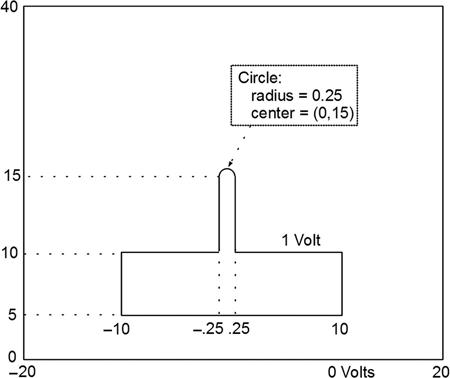
FIGURE 11.10 Structure using rectangles and a circle as electrodes.
Each line in the data file describes a particular electrode geometry. The entry in the first column of each line selects the geometry of that line. Currently allowed values of this entry are 1 — a horizontal line, 2 — a vertical line, and 3 — a circle. Each line has a total of five entries. The table below summarizes the available geometries:
| Column1 | Column2 | Column 3 | Column 4 | Column 5 |
| Horizontal line | Y location | Leftmost X | Rightmost X | Voltage |
| Vertical line | X location | Lower Y | Upper Y | Voltage |
| Circle | Radius | Center X | Center Y | Voltage |
Figure 11.11 shows the results of a ppt4.m run using the data file data1.txt. The electric field (Ey above the post) was calculated from the voltage data using the simple finite difference derivative approximation. Superimposed on the data is the result of a curve fit to these data using the function
Several observations about this program run and the results are described here:
- The convergence criterion [equation (11.12)] does not apply in this program because of the continual readjustment of the step size. For the results shown, a fixed number of iterations (50,000) was used at each starting point.
- The curve fit is, of course, not unique. The results “look pretty good” but this is hard to quantify.
- The results are very noisy. We can use these results to learn about the electrostatic nature of the system, but much more refined runs are necessary if quantitative results are desired.
- The results (and the curve fit) demonstrate the peaking of an electric field at the tip of a post, and the falling back of the electric field to background level as we move away from the post.
The PPT method allows for an interesting interpretation of the peaking of electric fields near sharp objects. Consider the three cases shown in Figure 11.12.
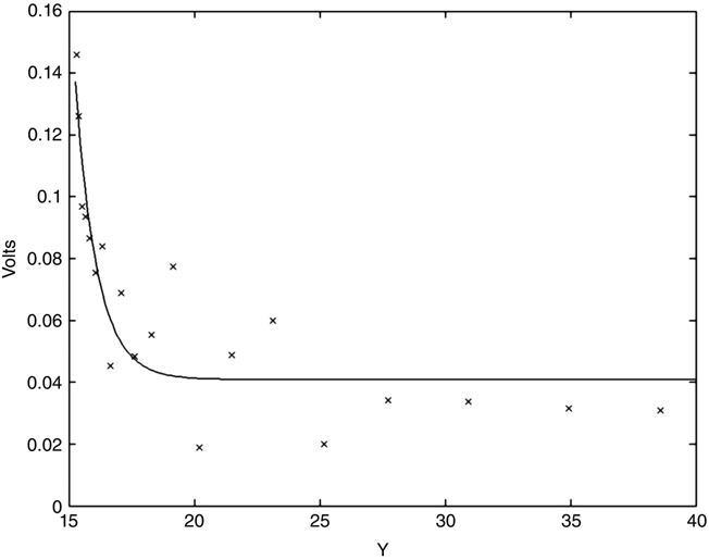
FIGURE 11.11 ppt4.m results for data1.txt dataset.
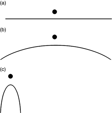
FIGURE 11.12 Examples of various degrees of sharpness near a field point.
In all of the three cases depicted in Figure 11.12, the black dot represents a point where we are calculating the voltage. Along the line normal to the surface and passing through the point, our best estimate of the electric field is

where V(0) is the known applied voltage (boundary condition) on the conductor and V(h) is the voltage predicted by the calculation.
In the case of Figure 11.12a, particles beginning to wander randomly from the point have a high probability of reaching the nearby electrode surface (a plane in this case). This implies that V(h) would be close to V(0) and Ey would be small.
In the case shown in Figure 11.12b, the wandering particles would be less likely to hit the electrode surface before wandering off and possibly hitting another surface. Assuming that the other surface is at a different potential than V(0) (e.g., the outside box in our previous example), the field would be somewhat higher than it was in Figure 11.12a.
In the case in Figure 11.12c, the particles will most likely miss the nearby electrode and wander off. In this case the voltage would be closer to the outside box voltage (in our previous example) than to the nearby electrode voltage, and the field would be very high. The sharper the tip and the higher it sits on a post and base electrode of the same voltage, the less likely that the particle will find this compound electrode structure, and consequently the higher the electric field will be.
11.5 Three-Dimensional Structures
Extending the gridless approach to three dimensions is straightforward — the probability of a step is now ![]() for the six orthogonal choices. One issue that must be contended with is that finding the closest point on some surface and choosing one step as the step to this point does not uniquely define all the steps as it did in two dimensions.
for the six orthogonal choices. One issue that must be contended with is that finding the closest point on some surface and choosing one step as the step to this point does not uniquely define all the steps as it did in two dimensions.
In Figure 11.13, (x 0,y 0) is the current point and p 1 is the closest point to the current point on one of the surfaces in the geometry. Whereas P 2 is now uniquely defined, the other four points are not uniquely defined. They are orthogonal to each other and to the lines from the current point to p 1 and p 2, and all six distances from the current point are the same. The four lines (from the current point to p 2–p 6) may be regarded as a rigid cross that can be spun about the line from p 1 to p 2. In this case a second random number should be obtained to determine the angle between, say, the line from the current point to p 2 and some fixed reference in the structure. Once this is chosen, all six points are specified.
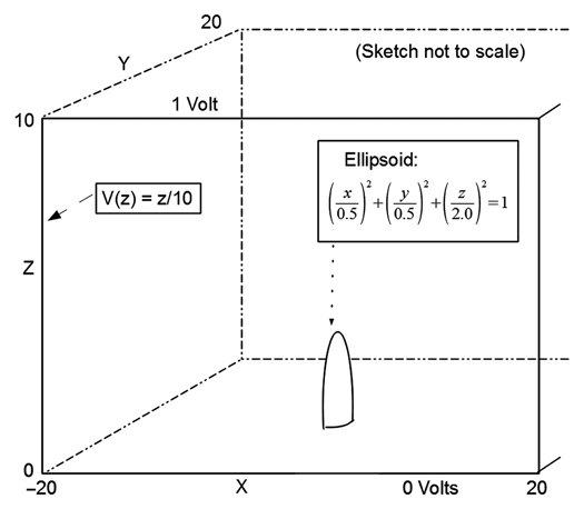
FIGURE 11.13 Example of three-dimensional gridless random-walk step generation.
Problems
11.1 Suppose that we want to use the gridded random-walk procedure (ppt1.m) to find all the node voltages in a structure. As the program stands, this is simply a job of rerunning the program with every free (nonboundary) node as the starting point (assuming, of course, that there are no symmetries in the structure to employ). Modify ppt1.m to do this and to store the results in a matrix V. In order to avoid excessive computer runtime, fix the number of iterations to 1000 per starting point.
11.2 Add the boundary conditions into the V matrix of Problem 11.1 and view the results using MATLAB'S mesh(x,y,V) function.
11.3 Calculate the 95% confidence interval at each matrix point voltage generated in Problem 11.1. View these results using the mesh function.
11.4 One way of improving (reducing) the computer runtime of Problem 11.1 is, as each node voltage is determined, to convert that node to a boundary condition fixed at this (now known) voltage. Modify the program written for Problem 11.1 (or simply create a new program) to do this. Compare the runtimes and the results of the two programs. Are there any new issues here?
11.5 Using ppt4.m, generate a dataset for two concentric cylinders (two circles in this 2d calculation), run the program, and compare the results to the exact answer.
11.6 Create a dataset for ppt4.m of a circle of radius 10 centered in an outer square of side(s) 40. Add a semicircle of radius 1 “sitting” on the original circle, centered at (0,10) as shown in Figure P11.6.
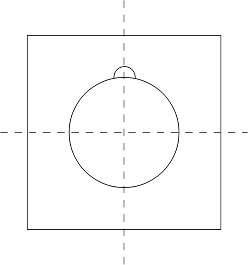
FIGURE P11.6 Geometry for Problem 11.6.
Set the outer square to 0 V and the circle and semicircle to 1.0 V. Calculate the voltage at several arbitrary points.
11.7 Starting with the program ppt4.m, add the capability for describing an ellipse in terms of its center and its major and minor axes. Since a general ellipse description requires four geometry parameters and the existing data structure allows for only three geometry parameters, we'll simplify the situation and require that the center of the ellipse be on the Y axis (X = 0). This guarantees backward capability with earlier datasets.

FIGURE P11.7 Structure for Problem 11.7.
For the structure shown in Figure P11.7, set the outer box at 0 V and the ellipses at 1 V, and calculate the V(y) at X = 0.
References
- 1. Brownian Motion,
www.wikipedia.com. - 2. Diffusion, Diffusion Equation,
www.wikipedia.com. - 3. R. Geulusee, Probabilistic potential theory applied to electrical engineering problems, Proc. IEEE 61(4): (April 1973).
- 4. L. Golnick and W. Smith, The Cartoon Guide to Statistics, HarperPerennial, New York, 1993.
- 5. L. Dworsky, Probably Not, Wiley, Hoboken, NJ, 2008.