
13
Triangles and Two-Dimensional Unstructured Grids
13.1 Introduction
Because the finite element method (FEM) is capable of handling complex geometries and different boundary conditions, much of its development occurred in the mechanical engineering community.3 Electrostatic applications of FEM are rarely as demanding in either the structural complexity or the boundary condition arenas as are many mechanical (stress–strain) problems, so the full menu of capabilities of FEM analysis will not be considered in this book.
The flexibility of using unstructured triangular cells was demonstrated using the method of moments (MoM) technique discussed earlier. In this chapter the use of unstructured triangular cells for planar two-dimensional (2d) FEM models will be developed. For MoM models, there was a good argument for working with right triangles — the barycenter of every triangle was of particular interest, and using right triangles facilitated the analyses. In FEM analysis there is nothing special about a right triangle, so triangles of any shape will be allowed.
Unstructured FEM grids are bookkeeping intensive. The computer program needs three sets of information:
- A List of Nodes. This list assigns a node number to each node and specifies its location.
- A List of Elements. When the elements are triangles, the list specifies each triangle and the (three) nodes that are their vertices.
- A List of Boundary Conditions. This list specifies which nodes are fixed or along planes of symmetry and, in the former case, the voltages at which these nodes are fixed.
There is no absolute “best way” to organize these lists. Lists 1 and 3 can be combined or kept separate.
Other than for very simple demonstration structures, FEM models are generated by computer. The computer software chosen to accomplish this task guides the design of the structure of the data file(s), as we will see shortly.
When calculating capacitance of an unstructured model, the total charge calculation is rarely used. This is due to the difficulty of drawing a satisfactory Gaussian surface. On the other hand, the stored energy calculation is very easy to implement.
Before looking at data structures, we need to derive the coefficient matrix entries for an arbitrary triangle.
13.2 Aside: The Area of a Triangle
This formula will be useful going forward. Figure 13.1 shows an arbitrary triangle (T) in the X–Y plane, inscribed in a rectangle.

FIGURE 13.1 Arbitrary triangle inscribed in a rectangle for area calculation.
The rectangle’s sides are parallel to the X and Y axes, and the vertices of triangle T is as shown. The area of T is simply the area of the rectangle minus the areas of right triangles A, B, and C:
After some manipulation, We obtain

The choice of which vertex is vertex 1, and so on is arbitrary, provided that the vertices are numbered counterclockwise. If they are numbered clockwise, the equation (13.2) calculates the negative of the area.
We will adopt the convention that all element vertices are numbered counterclockwise.
13.3 The Coefficient Matrix
Figure 13.2 shows the same triangle as in Figure 13.1, but without the surrounding rectangle.
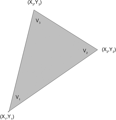
FIGURE 13.2 General triangle for analysis.
The three vertices are set to voltages V1, V2, and V3, as shown. The voltage anywhere in the triangle is given by the function
where the fi are the basis functions

and ai, bi, and ci are determined by the three sets of conditions


The electric field components are
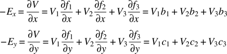
and then
Since the energy is not a function of x or y (in this approximation), we obtain

where AT is as given by equation (13.2).
The terms that must be added to the coefficient matrix (also called assembling the matrix) are obtained by setting the derivatives of equation (13.10), using (13.9), to zero:
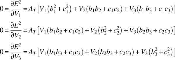
Comparing equations (13.10) and (13.11), it appears that the triangle area AT can drop out because of the 0 on the left side of equations (13.11). Remember, however, that here we are looking at only one triangle of an entire structure. We will sum the energy contributions from all triangles and then take derivatives and set them equal to zero. Except in the (possible but unlikely) case that all the triangles' areas are the same, the area terms will not drop out.
The coefficient matrix for an actual n node structure will have n rows, each row corresponding to a node. If the three nodes of the structure corresponding to the three nodes of the triangle T (Figure 13.2) are ni for the node at (xi,yi), then equations (3.11) become
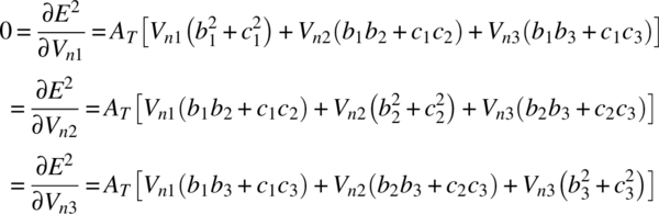
As an example, suppose that we have an eight-node system. The coefficient matrix a, is an 8 × 8 square matrix. Assume that we examine our node list and find that, for triangle 7, n1 is node 1, n2 is node 3, and n3 is node 4. We add the terms from equation (13.12) to the coefficient matrix as equal to

After this has been done for all of the triangles, it is necessary only to bring in the boundary conditions (in exactly the same way as was done for FD equations) and then solve the system for the node voltages.
Once the node voltages have been found, the voltage everywhere is known through equations (13.3)–(13.7), the electric field is known through equation (13.8) (using the coefficients found above). The energy stored in the electric field of each triangle is known through equations (13.10) and (13.9) (again, using the coefficients found above), and the total energy in the system is found by summing all of the individual triangles' energies.
13.4 A Simple Example
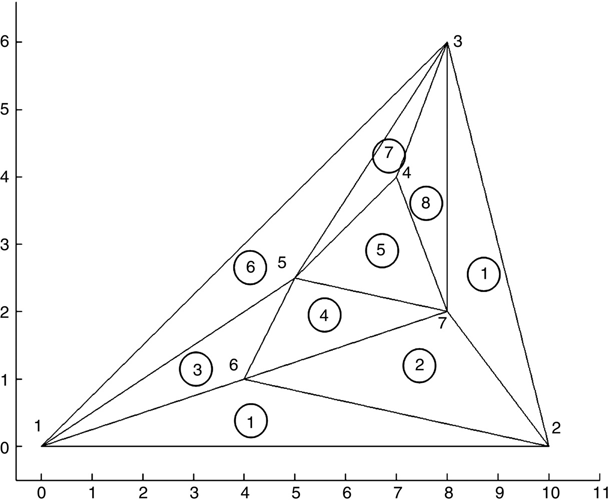
FIGURE 13.3 A very simple triangular mesh structure.
Figure 13.3 shows a very simple triangular mesh (of a triangular structure). This structure is of no particular interest for its electrostatic properties; its use is for illustrating the FEM file information and matrix assembly technique while being as simple as possible. It does have all of the characteristics of more complicated (and more interesting) structures. Examining Figure 13.3, we note that
- The structure is made up of nine triangles with seven common vertices, or nodes. The nodes are numbered using large numbers; the triangles are numbered using smaller, encircled, numbers.
- Each node has a number. The choice of node number (i.e., which node has which number) is arbitrary as long as each node is represented by a unique number, starting at 1, and no numbers are skipped.
- There is a closed outer boundary. These are the lines connecting nodes 1–2, 2–3, and 3–1.
- The nodes on the outer boundary will be set to a boundary condition (typically 0 V).
- There are four internal nodes. At least one of these will be set to a boundary condition other than 0 V. The remaining node voltages will be the unknown variables that we wish to find. We can, of course, set all of the internal nodes to a boundary condition, but then the voltage distribution is fixed and there are no voltages to find. We can still find the stored energy if it is of interest.
- All of the triangle locations are arbitrary so long as no triangle crosses over another triangle and no vertex of any triangle sits along a leg of another triangle.
- Each triangle has a unique number. The numbering choice is arbitrary, with the same constraints as the node numbering. There is, in general, no formula relating the number of triangles to the number of nodes or linking a triangle’s number to the node numbers of that triangle.
Our first task is to gather all the information about this structure, along with the boundary condition information, and put it in a form that’s easily readable by a computer program. Since we want to write programs that are reusable for multiple structures, this means that we want to create data files with all of the necessary information. There is no absolute best algorithm for doing this. The choice presented here is to create three files to carry the node location information, the triangle descriptions, and the boundary conditions.
Table 13.1 is a listing of the node information of this structure, nodes_debug.txt. The first column (italicized) is not actually part of the file. It is simply a counting list (row number) of the nodes. The computer program gets this information automatically as it reads the file; there is no need to explicitly show the counting in the data file. Columns 2 and 3, the actual data file, show the X and Y locations of each node.
TABLE 13.1 Node Information
| Node | X | Y |
| 1 | 0 | 0 |
| 2 | 10 | 0 |
| 3 | 8 | 6 |
| 4 | 7 | 4 |
| 5 | 5 | 2.5 |
| 6 | 4 | 1 |
| 7 | 8 | 2 |
Table 13.2 is a listing of the triangle information for this structure, triangles_debug.txt.
TABLE 13.2 Triangle Information
| Triangle | Nodes | ||
| 1 | 1 | 2 | 6 |
| 2 | 6 | 2 | 7 |
| 3 | 1 | 6 | 5 |
| 4 | 6 | 7 | 5 |
| 5 | 5 | 7 | 4 |
| 6 | 5 | 3 | 1 |
| 7 | 5 | 4 | 3 |
| 8 | 4 | 7 | 3 |
| 9 | 7 | 2 | 3 |
Again, the first (italicized) column is not actually part of the file; it is simply a counting list (indicating row number of the triangles). Columns 2–4 list the three nodes that are the vertices of the triangles. The order of the node numbering for each triangle is arbitrary as long as they are ordered counterclockwise for each triangle.
Table 13.3 is a listing of the boundary condition (bc) information file bcs_debug.txt. The format of this file is, at this point, not totally logical. Column 1 (italicized) conveys no necessary information; it is included for forward compatibility with the automatic meshing capability to be introduced in Chapter 14. For the moment, simply ignore column 1.
TABLE 13.3 Boundary Condition Information
| Ignore | Node | bc |
| 1 | 1 | 0 |
| 1 | 2 | 0 |
| 1 | 3 | 0 |
| 1 | 5 | 1 |
| 1 | 6 | 1 |
Columns 2 and 3 comprise a list of the nodes that are to be boundary conditions and the voltage to which these nodes are set, respectively. Referring to Figure 13.3, the three outer boundary nodes (1, 2, and 3) are set to 0 V and two of the internal nodes (5 and 6) are set to 1 V.
13.5 A Two-Dimensional Triangular Mesh Program
The MATLAB program fem_2d_1.m reads the data files described above, assembles the matrices, finds the node voltages and the structure’s capacitance, and produces some useful graphics. It was written “looking forward” to provide compatibility with the more complicated problems presented in Chapter 14, so some pieces of the code are at this point unnecessary; this will be pointed out as needed:
- Program
fem_2d_1.m—2d triangular mesh FEM program:% 2d FEM with triangles close all filename = input('Generic name for input files: ', 's'), nodes_file_name = strcat('nodes_', filename, '.txt'), trs_file_name = strcat('trs_', filename, '.txt'), bcs_file_name = strcat('bcs_', filename, '.txt'), % get node data dataArray = load (nodes_file_name); nds.x = dataArray(:, 1); nds.y = dataArray(:, 2); nds.z = 0; nr_nodes = length(nds.x) % get triangles data trs = (load(trs_file_name))'; nr_trs = length(trs) % get bcs data bcs = get_bcs(bcs_file_name); dataArray = load(bcs_file_name); bcs.node = dataArray(:,2); bcs.volts = dataArray(:,3); nr_bcs = length(bcs.node) % allocate the matrices a = sparse(nr_nodes, nr_nodes); f = zeros(nr_nodes,1); b = zeros(3,nr_nodes); c = zeros(3,nr_nodes); % generate the matrix terms d = ones(3,3); for tri = 1: nr_trs % Walk through all the triangles n1 = trs(1,tri); n2 = trs(2,tri); n3 = trs(3,tri); d(1,2) = nds.x(n1); d(1,3) = nds.y(n1); d(2,2) = nds.x(n2); d(2,3) = nds.y(n2); d(3,2) = nds.x(n3); d(3,3) = nds.y(n3); Area = det(d)/2; temp = d[1; 0; 0]; b(1,tri) = temp(2); c(1,tri) = temp(3); temp = d[0; 1; 0]; b(2,tri) = temp(2); c(2,tri) = temp(3); temp = d[0; 0; 1]; b(3,tri) = temp(2); c(3,tri) = temp(3); a(n1,n1) = a(n1,n1) + Area*(a(n1,n1) + b(1,tri)^2 + c(1,tri)^2); a(n1,n2) = a(n1,n2) + Area*(a(n1,n2) + b(1,tri)*b(2,tri) + c(1,tri)*c(2,tri)); a(n1,n3) = a(n1,n3) + Area*(a(n1,n3) + b(1,tri)*b(3,tri) + c(1,tri)*c(3,tri)); a(n2,n2) = a(n2,n2) + Area*(a(n2,n2) + b(2,tri)^2 + c(2,tri)^2); a(n2,n1) = a(n2,n1) + Area*(a(n2,n1) + b(2,tri)*b(1,tri) + c(2,tri)*c(1,tri)); a(n2,n3) = a(n2,n3) + Area*(a(n2,n3) + b(2,tri)*b(3,tri) + c(2,tri)*c(3,tri)); a(n3,n3) = a(n3,n3) + Area*(a(n3,n3) + b(3,tri)^2 + c(3,tri)^2); a(n3,n1) = a(n3,n1) + Area*(a(n3,n1) + b(3,tri)*b(1,tri) + c(3,tri)*c(1,tri)); a(n3,n2) = a(n3,n2) + Area*(a(n3,n2) + b(3,tri)*b(2,tri) + c(3,tri)*c(2,tri)); end % bcs for i = 1: nr_bcs n = bcs.node(i); a(n,:) = 0; a(n,n) = 1; f(n) = bcs.volts(i); end % Non-mesh nodes: Set up phony voltage just for matrix form for i = 1 : nr_nodes if a(i,i) == 0 a(i,:) = 0; a(i,i) = 1; f(i) = 0; end end v = af; % calculate capacitance C = get_tri2d_cap(v, nr_nodes, nr_trs, nds, trs) % plot the mesh show_mesh(nr_nodes, nr_trs, nr_bcs, nds, trs, bcs, v) - Program
get_tri2d_cap.m:function C = get_tri2d_cap(v, nr_nodes, nr_trs, nds, trs) % Calculate the capacitance of a 2d triangular structure % Simple linear approx. function is assumed eps0 = 8.854; U = 0; d = ones(3,3); for tri = 1 : nr_trs n1 = trs(1,tri); n2 = trs(2,tri); n3 = trs(3,tri); d(1,2) = nds.x(n1); d(1,3) = nds.y(n1); d(2,2) = nds.x(n2); d(2,3) = nds.y(n2); d(3,2) = nds.x(n3); d(3,3) = nds.y(n3); temp = (d[1; 0; 0]); b1 = temp(2); c1 = temp(3); temp = (d[0; 1; 0]); b2 = temp(2); c2 = temp(3); temp = (d[0; 0; 1]); b3 = temp(2); c3 = temp(3); Area = det(d)/2; if Area < = 0, disp 'Area < = 0 error'; end; U = U + Area*((v(n1)*b1 + v(n2)*b2 + v(n3)*b3)^2 … + (v(n1)*c1 + v(n2)*c2 + v(n3)*c3)^2); end U = U*eps0/2; C = 2*U; % Potential difference of 1 volt assumed end - Program
show_mesh.m:function show_mesh(nr_nodes, nr_trs, nr_bcs, nds, trs, bcs, v) % Take a look at the input data and the solution x_min = min(nds.x)*1.1; if x_min == 0, x_min = -.5; end; x_max = max(nds.x)*1.1; y_min = min(nds.y)*1.1; if y_min == 0, y_min = -.5; end; y_max = max(nds.y)*1.1; figure(1) axis ([x_min, x_max, y_min, y_max]); hold on for i = 1 : nr_trs n1 = trs(1,i); n2 = trs(2,i); n3 = trs(3,i); x = [nds.x(n1), nds.x(n2), nds.x(n3), nds.x(n1)]; y = [nds.y(n1), nds.y(n2), nds.y(n3), nds.y(n1)]; plot (x,y, 'k') end hold on for i = 1 : nr_bcs n = bcs.node(i); x = nds.x(n); y = nds.y(n); text (x, y, num2str(bcs.volts(i))) end figure(2) axis ([x_min, x_max, y_min, y_max]); for i = 1 : nr_trs n1 = trs(1,i); n2 = trs(2,i); n3 = trs(3,i); x = [nds.x(n1); nds.x(n2); nds.x(n3)]; y = [nds.y(n1); nds.y(n2); nds.y(n3)]; z = [v(n1); v(n2); v(n3)]; colormap (gray) % Delete this line for color graphics fill (x,y,z) hold on end end
The program begins by requesting the name for the data files, in this case debug. It then reads the three data files described in Section 13.4.
Matrix assembly and equation solution follow the analysis directly. The boundary conditions are inserted in exactly the same manner as was done in the FD analysis.
The lines beginning with the comment (fake bcs …) do nothing in this example. The purpose of these lines of code will be explained in Chapter 14.
The capacitance of the structure is calculated by the function get_tri2d_cap.m. The stored energy is calculated directly from the equations above.
Function show_mesh.m produces two graphs. The first of these, Figure 13.4, is a sketch of the structure as understood by the program. This is useful for verifying that the data files are correct. Also, the function puts the voltage boundary conditions at the appropriate nodes. Again, this is useful for verifying that the problem is being correctly set up.

FIGURE 13.4 Sketch of structure and boundary conditions as understood by the computer.
The second graph produced is again a sketch of the structure, but this time the voltage profile is interpreted as shades of gray or color. Deleting line noted in the function show_mesh.m changes the MATLAB color map from gray shades that were needed for black-and-white Figure 13.5 (black = 0 V, white = 1 V) to more visually interesting colors, which vary from blue = 0 V to red = 1 V.
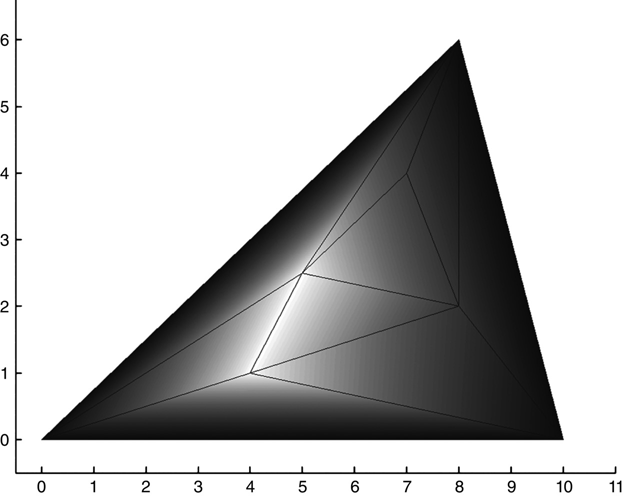
FIGURE 13.5 Sketch of structure and grayscale map of voltage profile.
Inspection of these figures should verify the boundary condition voltages and provide a visual image of the voltage profile that both passes a commonsense test and gives some insight (when dealing with real structures) of the voltages involved.
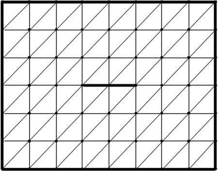
FIGURE P13.4 Structure for Problem 13.2.
Problems
- 13.1 Write a simple MATLAB script to create the data files for the structure shown in Figure P13.1 (or use a spreadsheet, do it manually, etc.). Run
fem1_2d.mand verify that the data files are correct by inspecting the graphics and the resulting capacitance. Does the voltage profile generated look reasonable? - 13.2 Modify the data files produced for Problem 13.1 to create the structure shown in Figure P13.4. Comment on the results of using this data file in
Prob13_1.m(as compared to the previous results).
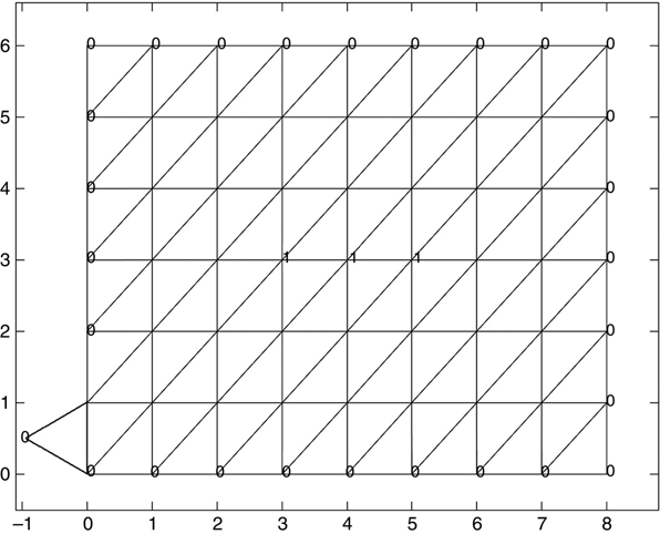
FIGURE P13.1 Structure for Problem 13.1.
- 13.3 Modify the data files produced for Problem 13.2 to create the structure shown in Figure P13.5.
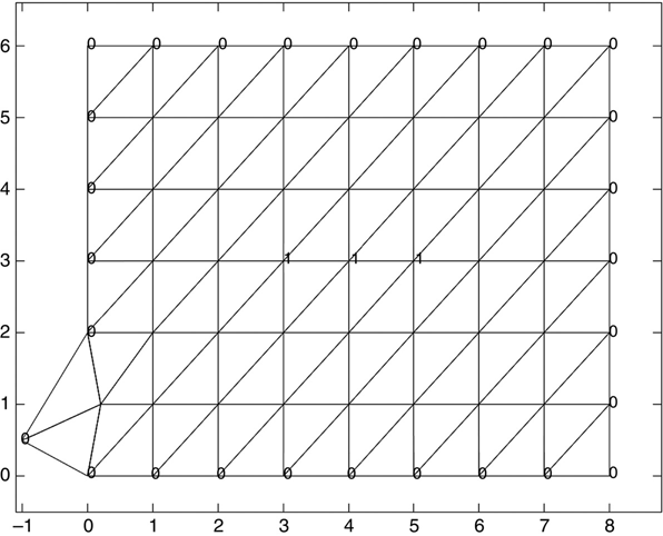
FIGURE P13.5 Structure for Problem 13.3.
- 13.4 Program
fem2d_1.mwill provide the basis of the working programs for the next few chapters. Readers intending to use the programs to solve real problems, or as the bases of programs to solve real problems, and who are familiar with vectorizing MATLAB program techniques, should consider vectorizingfem2d_1.mas a good problem, or project.
Reference
- 1. O. C. Zienkiewicz and R. L. Taylor, The Finite Element Method, 6th ed., Elsevier Butterworth-Heinemann, Burlington, MA, 2005.