
6
Triangles
6.1 Introduction to Triangular Cells
All of the examples and calculations presented thus far have been based on the use of rectangular cells in an X–Y plane. Rectangular cells in an X–Y plane are very useful for many practical problems, so this wasn’t a bad choice. However, rectangular cells are very awkward to work with in three-dimensional (3d) structures, especially when the surfaces involved are not planar. A good example of this problem is the surface of a sphere; there is simply no convenient way to approximate the surface of a (conducting) sphere using a collection of rectangular cells. Also, when a structure has regions where smaller cells are needed to resolve complex geometric features and/or accurate approximate regions where the electric field is changing rapidly but larger cells are satisfactory for much of the geometry, the programs presented in Chapters 1 and 3–5 seldom can do the job — they were written to be as simple as possible and used square cells. A much more useful choice is triangular cells of arbitrary size, location, and orientation. Also, and finally, readers by now must be wondering whether there isn't more to electrostatics than transmission line sections.
Restricting ourselves to uniform-size rectangular cells in X–Y planes let us develop basic method of moments (MoM) solution techniques for different situations (images, dielectric interfaces, rotated electrodes, etc.) and look at solutions without being distracted by complexities of processing geometric information. The get_data_xxx.m functions presented in Chapters 4 and 5 translated two- or three-line input files to all the necessary cell information in only a few lines of code. Moving on to triangles of arbitrary size location and orientation in 3d space brings with it a lot of programming baggage that must be layered on top of the basic algorithm of describe geometry — calculate Li,j — solve the linear equation set. Unfortunately, there is no way around this.
Approximating a surface with triangular (or other) regions is called tessellation. Generating tessellations in two dimensions for MoM problems or in two or three dimensions for finite element or other techniques is a sophisticated field into itself, and there are many texts describing many techniques as well as many software packages available. A full discussion of this subject is outside the scope of this book and won’t be delved into deeply here. Instead, in this chapter we’ll work with existing MATLAB capability and a freely available package that, together, give us a very versatile and powerful capability. The calculations to be described are correct regardless of how the cell structure was created, so these discussions are not limiting in any sense.
6.2 Right Triangles
Limiting our mathematics to right triangles simplifies the work to be done. As shown in Figure 6.1a, any triangle can be subdivided into two right triangles by drawing a line from the vertex opposite the longest side to the longest side, at a 90o angle to the longest side.

FIGURE 6.1 Right triangles.
In the case of a triangle with two equal longest sides or three equal sides, the choice is arbitrary.
Consider any right triangle, rotated so that its legs are parallel to the X and Y axes (Figure 6.1b). The leg parallel to the X axis is of length a, the leg parallel to the Y axis is of length b. It can easily be shown that the three lines drawn from each vertex to the midpoint of the opposite side intersect at the common point (a/3, b/3). This point is the barycenter,1 that is, the center of mass, of the right triangle—regardless of the values of a and b. If we assume that all the charge is concentrated at this point (the long-distance approximation for Li,j ), then the odd-order moments cancel,2 making this the best choice for this point.
Note that the center of a rectangle is its barycenter, due to the symmetries of the rectangle, so no problems arose with rectangles and there was no need to mention this consideration earlier.
Going forward, assume that every triangle (other than right triangles themselves) that is used to describe an electrode geometry will be broken into two right triangles and that there can then be up to twice as many cells (variables) in the numerical problem as there are in the geometric description. If the initial triangles (number, sizes, and positions) have been well chosen to describe the problem, then these subdivisions will not degrade the quality of the model.
6.3 Calculating L i,i (Self) Coefficients
Figure 6.2 shows the right triangle of Figure 6.1 translated so that the barycenter of the triangle is at the origin of the axes. Note that there has been no rotation—sides a and b are still parallel to the X and Y axes, respectively. The triangles of Figures 6.2 and 6.1 look different; this was done deliberately to emphasize the point that the definitions of a and b are consistent in both figures and the calculations below will always be correct, regardless of the relative sizes of a and b. This is not the same as saying that values of a and b are not important.

FIGURE 6.2 Layout for calculating Li,i for a right triangle.
Without any loss of generality, Li,i is the voltage at (0,0) due to a uniform charge distribution on the triangle with a total charge of Qi :

where the integral is over the area of the triangle.
Switching to polar coordinates and substituting the area of the triangle, we obtain
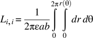
Referring to Figure 6.2, the three angles shown are, in terms of a and b, as follows:
The entire triangle is then divided into the three regions
The integrals in these three regions are
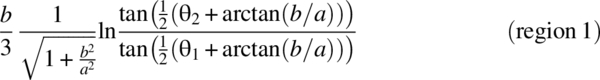
At this point it is straightforward to substitute the angle definitions into equations (6.10)–(6.12), sum the three results, and get the final expression for Li,i . The resulting expression, however, is so messy that it would take at least half of the page to write it out. Since there is very little doubt that anyone needing this expression will generate the numbers using computer code, it is just as useful to leave things as they are. Starting with a and b, calculate the three angles using equations (6.4), (6.5), and (6.6); substitute these angles into equations (6.10), (6.11), and (6.12); and add the three resulting numbers together to obtain the value of the integral in equation (6.3).
6.4 Calculating L i,j FOR i ≠ j
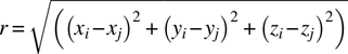
As in the case of rectangles, we cannot integrate the general expression for Li,j . Following the same procedure as in the case of rectangles to develop an approximate expression, the following expression gives good results. Let j represent the charged (right) triangle with (xj ,yj ,zj ) as its barycenter. Let (xi ,yi ,zi ) be the field point at which we want the voltage (in the case, the barycenter of triangle i).
Let
Then
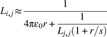
where
6.5 Basic Meshing and Data Formats for Triangular Cell MoM Programs
Our modeling program using triangular cells in principle parallels the rectangle program(s), but there are now many more tasks to complete. Some of these tasks are due to the use of triangles, and some of them are necessary because, unlike the previous constraint that all electrodes be in an X–Y plane, we’re eliminating all constraints on electrode location and orientation.
A good user-oriented modeling program would take the issue of data validation very seriously. For example, are we accidentally specifying that one electrode, at some voltage, passes through or lies on top of another electrode at some other voltage? For our purposes this is extra programming; it contributes neither to understanding of the electrostatics or modeling nor to the results. In general, ignoring this task is a poor decision; it is being made here to try and keep a large task from becoming an overwhelming task for a newcomer.
Going forward, task 1 consists of generating triangular element surfaces that represent the geometry we wish to model. Since the results of this task are not unique, we must make some decisions in addition to the basic “how much resolution do we need — aka what is the value of a?” choice that came up in the previous models.
For example, Figure 6.3 shows a simple handmade right triangle mesh of a planar square electrode. There is a possible problem, however. While both the upper left and lower right triangles fill the corners the same way and the upper right and lower left triangles fill the corners the same way, all four corners are certainly not treated similarly. If we were to build a capacitor using two identical planar squares, we would probably get a good calculation of capacitance, but what about the fields and charge densities in the corners? Physically we know that they should be identical, but would they be identical?
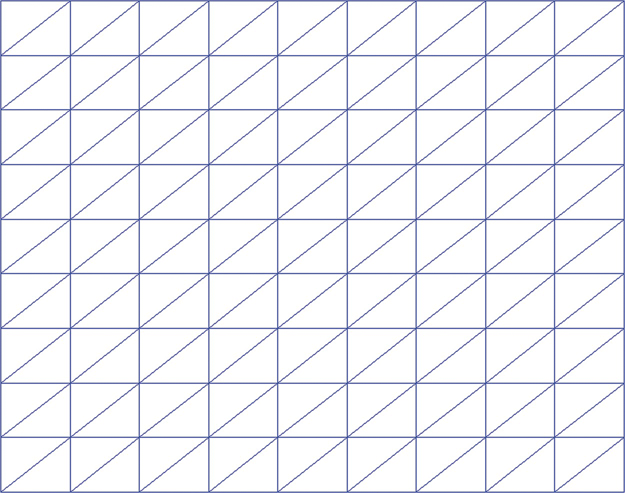
FIGURE 6.3 Simple hand meshing of a square planar electrode.
Figure 6.4 shows a more complicated structure. This mesh was generated using a software package that will be presented later. The configuration of the drawing has been changed from that in Figure 6.3. Because we might now consider electrode surfaces with holes (and/or irregular outer boundaries) the actual electrode region is shown in gray; this makes an internal hole very visible.
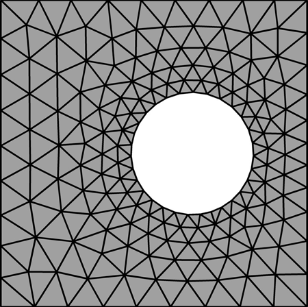
FIGURE 6.4 Meshing of a planar square electrode with an off-center hole.
This electrode has been set up so that the hole is off-center in the square and the resolution near the hole is higher than elsewhere. Now we have to make not one, but several, decisions about resolution.
Figure 6.5 shows a meshed sphere surface. All of the triangles are not identical. Even when unwanted, this happens sometimes because the geometry is not amenable to identical triangular meshing and sometimes the generation software just can't figure out how to do it. In the case of concentric spherical electrodes, for example, we know that physically the charge density on both spheres must be absolutely uniform; however, the model will show small but noticeable variations. This means that we must consider cell size and the expected limits of resolution.
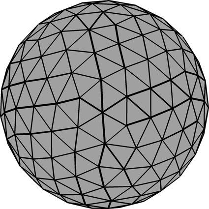
FIGURE 6.5 Uniformly meshed sphere.
The program mom_tri_1.m is presented here to demonstrate a triangular cell script:
% mom_tri_1.m script for solving triangular cell mom problems

clear

% This is a first pass test program to demonstrate all the routines
% necessary to model triangles
% Each row in the array all_tris is a triangle that is, going forward,
% brought in from the mesh generator(s).
% Cols 1:3 is the first node (arbitrary) point (nx1,ny1,nz1)
%     4:6      2nd (nx2,ny2,nz2)
%     7:9      3rd (nx3,ny3,nz3)
%     10 is the voltage the triangle is set to


% This data file is hand-generated and written into the routine
all_tris  =          [-.5   0  0   1    0  0  1   2  0  .5];  % #1
all_tris  = [all_tris;  [-.5  0  0   1   2  0  -.5  2  0  .5]];   % #2
all_tris  = [all_tris;  [-1   0  1   1   0  1  1.5   1    1. -.5]];  % #3
all_tris  = [all_tris;  [-1   0  1   1.5   1  1  0   1  1   -.5]]; % #4


q = triangles_1(all_tris);


V_off = q(end)
q = q(1:end-1)
C1 = sum(q.*(q > 0))
C2 = sum(q.*(q < 0))
MATLAB program mom_tri_1.m is a simple demonstration script for setting up and solving a method of moments (MoM) problem using triangular cells. This program includes two input electrodes, each composed of two triangles. These triangles are shown in Figure 6.6.

FIGURE 6.6 Triangles described in mom_tri_1.m.
In Figure 6.6 the triangles are numbered according to their order in the computer file. The lines in the file can appear in any order without affecting the results. The program mom_tri_1.m (a utility program for triangular cell MoM modeling) calls triangles_1.m and passes the triangle information (all_tris) to it.
function [q, rt_tris] = triangles_1(all_tris)


 %  triangles_1.m


 [nr_input_tris,p] = size(all_tris);
 fprintf ('Number of triangles in input file = %d
', nr_input_tris)


% INPUT DATA VERIFICATION SHOULD OCCUR HERE IN A REAL WORKHORSE PROGRAM


% Generate right triangles from the data
 [rt_tris, volts] = make_right_tris(all_tris);


 tic
 L =  get_L_2(rt_tris);  % vectorized
 nr_vars = length(L);
 new_col = ones(nr_vars,1);
 L =  [L, new_col];
 new_row = [new_col',0];
 L =  [L; new_row];
 toc


 % Solve and finish


 volts = [volts;0];
 q = Lvolts;


end
Program triangles_1.m is a utility program for calling other programs and performing some minimal file processing. It immediately calls make_right_tris.m, passing the triangle data (all_tris) to it. Ultimately this returns an array of right triangles (right_tris) and a vector of triangle voltages (volts).
The make_right_tris.m program — which provides a function for translating a triangle data file to an all-right-triangle data file — is as follows:
function [right_tris, volts] = make_right_tris( all_tris )
% Reads the all_tris list line by line and then splits every
%  triangle into two right triangles. An incoming right
%  triangle is just passed along


 right_tris = [];  volts = [];
 [nr_input_tris,p] = size(all_tris);
 for i = 1: nr_input_tris
  % nodes and voltage of the ith input triangle
  nodes = [all_tris(i,1:3);  all_tris(i,4:6);  all_tris(i,7:9)];
  v = all_tris(i,10);


  [angs,nodes] = get_included_angles(nodes);  % get all the included angles
  if abs(sum(angs) - pi) > .01*pi   % check for problems
   fprintf ('Sum of angles error in triangle %d
', i)
  end
  % If triangle i already a right triangle, just add it to the list
  if (abs(angs(1) - pi/2) < .001*pi/2)
   right_tris = [right_tris; [nodes(1,:), nodes(2,:), nodes(3,:)]];
   volts = [volts;v];
  else
  % find the point for the new right angle vertices
   s21 = sqrt(sum((nodes(2,:) - nodes(1,:)).^2));
   s32 = sqrt(sum((nodes(3,:) - nodes(2,:)).^2));
   f = s21/s32*cos(angs(2));
  % create the new node and new triangles
   new_node = nodes(2,:) + f*(nodes(3,:) - nodes(2,:));
   right_tris = [right_tris; [new_node, nodes(2,:), nodes(1,:)]];
   right_tris = [right_tris; [new_node, nodes(3,:), nodes(1,:)]];
   volts = [volts;v]; volts = [volts;v];


  end
 end
end


% -----------------------------------------------------


function [angs, nodes] = get_included_angles(nodes)


 angs = [];  % get the included angles, return biggest as first
 v12 = nodes(2,:) - nodes(1,:);
 s12 = sqrt(sum(v12.^2));
 v13 = nodes(3,:) - nodes(1,:);
 s13 = sqrt(sum(v13.^2));
 dot = sum(v12.*v13);
 angs = [angs,acos(dot/s12/s13)];
 v21 = -v12;
 s21 = s12;
 v23 = nodes(3,:) - nodes(2,:);
 s23 = sqrt(sum(v23.^2));
 dot = sum(v21.*v23);
 angs = [angs,acos(dot/s21/s23)];
 v31 = -v13;
 s31 = s13;
 v32 = -v23;
 s32 = s23;
 dot = sum(v31.*v32);
 angs = [angs,acos(dot/s31/s32)];
 [ang_max, index] = max(angs);
 if index == 2
  temp = nodes(2,:);
  nodes(2,:) = nodes(1,:);
  nodes(1,:) = temp;
  temp2 = angs(2); angs(2) = angs(1); angs(1) = temp2;
 elseif index == 3
  temp = nodes(3,:);
  nodes(3,:) = nodes(1,:);
  nodes(1,:) = temp;
  temp2 = angs(3); angs(3) = angs(1); angs(1) = temp2;
 end


end
The make_right_tris.m program performs several operations on the all_tris array. Each line of all_tris describes a triangular electrode and the voltage on it. For each line of all_tris, the make_right_tris.m program performs the following tasks:
- Splitting the nine (9) geometry numbers into a 3×3–node array, each row containing the (x,y,z) information for one of the triangle's nodes (arbitrarily ordered at this point).
- Calling the
get_included_anglesarray, which calculates a 1×3 array of the included triangle angles, corresponding to the three nodes. It then rearranges the order of both the angles and node arrays so that the largest angle (and corresponding node) is first. - Adding up the angles and ensuring that they sum to π. (This was actually a debugging check during program development, but it can’t hurt to leave it in.)
- Creating a row in
all_tris[ifangs(1) = π/2, this is already a right triangle] with the node information and an entry in the volts vector with the voltage information. It then loops to the next triangle. -
Finding the point on the longest side, which, when connected to vertex 1, creates two right triangles. With reference to Figure 6.6, using the notation Ni = (xi ,yi ,zi ), we obtain
and so on. The new node, N 4, is given by
(6.17)
where 0 < f <1, f is yet to be determined. From Figure 6.7 and equation (6.17), we obtain
Therefore
- Adding the two new right triangles, (N
4,N
1,N
2) and (N
4,N
1,N
3), to the
rt_trianglesarray and add the voltage (twice) to the volts vector.

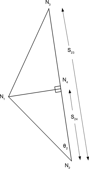
FIGURE 6.7 Arbitrary triangle split into two right triangles.
The program get_L_1.m—a first-pass L calculation program—is as follows:
function [L] = get_L_1(rt_tris )
%Generate the L array from the right triangles
 eps0 = 8.854;
 [nr_rt_tris,junk] = size(rt_tris);
 fprintf('Number of right triangles = %d
', nr_rt_tris)
 L = zeros(nr_rt_tris,nr_rt_tris); % allocate L array


 for j = 1: nr_rt_tris % j triangles are the charged triangles
  a = sqrt(sum((rt_tris(j,4:6) - rt_tris(j,1:3)).^2));
  b = sqrt(sum((rt_tris(j,7:9) - rt_tris(j,1:3)).^2));
  scl = (a + b)/4.; % empirical fitting function parameter
  err_check = (a^2 + b^2 - sum((rt_tris(j,7:9) - rt_tris(j,4:6)).^2)) …
      /(a^2 + b^2) ;
  if abs(err_check) > 1.e-3
   fprintf ('Right triangle file error, #%d %g
', j, err_check)
  end
  % barycenter of jth rt tri
  bary_jth = (rt_tris(j,1:3) + rt_tris(j,4:6) + rt_tris(j,7:9))/3;


  th1 = -atan(b/2/a);
  th2 = pi - atan(2*b/a);
  th3 = 3*pi/2 - atan(b/a);


  t1 = b/3/sqrt(1 + b^2/a^2)*log(tan(.5*(th2 + atan(b/a)))/tan(.5*(th1 + atan(b/a))) );
  t2 = -a/3*log(tan(th3/2 + pi/4.)/tan(th2/2 + pi/4.));
  t3 = -b/3*log(tan(th1/2)/tan(th3/2));


  L_self_tri = (t1 + t2 + t3)/(2.*pi*eps0*a*b);


  for i = 1: nr_rt_tris % this is the field point
   bary_ith = (rt_tris(i,1:3) + rt_tris(i,4:6) + rt_tris(i,7:9))/3;
   % barycenter - barycenter distance
   r = sqrt(sum((bary_ith - bary_jth).^2));
   L(i,j) = 1/(4*pi*eps0*r + 1./L_self_tri./(1 + r/scl));
  end
 end
end
The triangles_1_.m program passes the rt_tris array to get_L_1.m, which generates the L matrix. The get_L_1.m program is straightforward and follows the get_L routines presented in previous chapters. Calculating the self- (diagonal) L term is much more involved than it was for rectangles, but this is just a bookkeeping task for the computer. The get_L_1.m program has been written with explicit looping through all of the L matrix terms. This was done for clarity, certainly not for runtime efficiency. This issue will be addressed in Section 6.6.
The rest of the program is identical to the rectangle programs — the extra row and column needed to ensure charge neutrality are added to the L array, the set of linear equations is solved for q, and capacitance is calculated. For this simple dataset, the result is that C = 40.7 pF.
6.6 Using MATLAB to Generate Triangular Meshings
The example in Section 6.5 was complete in that it started with a description of the desired electrode geometry and ended up with a completed calculation of the charge distribution on the electrodes. Generating the triangle descriptions by hand, however, does not allow for interesting geometries. Although not an impossible task, manual generation of triangular meshings very quickly becomes an overwhelming task when the electrode geometries and desired resolutions are not trivial.
Fortunately, MATLAB has built-in capabilities that perform this task very well. Consider the mom_tri_2.m program, which presents a triangular cell script for basic MATLAB data generation:
% mom_tri_2.m script for solving triangular cell mom problems


close all; clear


all_tris = mesh_prob_6_5;
[q, rt_tris] = triangles_1(all_tris);


V_off = q(end)
q = q(1:end-1);
C1 = sum(q.*(q > 0))
C2 = sum(q.*(q < 0))


figure (2)
hold on
y = 0;


for z = 1 : .1 : 1.51
 x_plot = []; v_plot = [];
 for i = 0 : 100
  x = (i/100);
  x_plot = [x_plot, x];
  pt = [x,y,z];
  v_plot = [v_plot, get_V(pt,rt_tris,q)];
 end
 plot(x_plot, v_plot)
end


axis ([0 1 -.05 .55])
H = line ([.5 .5], [0, .5]);
set(H, 'Linestyle', '- -')
xlabel ('(X,Y,Z) = (X,0,0)')
ylabel ('Volts')
The mom_tri_2.m program is a simple modification of mom_tri_1.m. The explicit definition of the all_tris array has been replaced by a call to the function mesh_gen_1.
The mesh_gen_1.m program — which provides a function for generating and displaying the basic meshing procedure — is as follows:
function all_tris = mesh_gen_1
% mesh_gen_1.m first pass generated triangles data from Matlab routine


 test = [-0.5 : .07 : .5];
 [x,y] = meshgrid(test);
 %h = 1.0;  z = 0*x + h;     % flat electrode example
 h = 1.5;  z = 0*x + h;     % Gaussian Tip example


 tri = delaunay(x,y);   % generate triangles
 nr_tris = length(tri);


 trimesh(tri,x,y,z)


 all_tris = [];       % generate all_tris array
 V = 0.5;
 for i = 1:nr_tris
  n = tri(i,:);
  t1 = [x(n(1)), y(n(1)), z(n(1))];
  t2 = [x(n(2)), y(n(2)), z(n(2))];
  t3 = [x(n(3)), y(n(3)), z(n(3))];
  all_tris = [all_tris; [t1, t2, t3, V]];


 end


 %C = [.5,.5,.5; .5,.5,.5; .5,.5,.5];  % insert for b&w graphics
 %colormap(C)               % insert for b&w graphics
 axis ([-.75 .75 -.75 .75 0. 1.6])
 hold on


 % ---- bottom electrode --------------------------------------
 %h = 0.0; z = 0*x + h; % flat electrode example


 % improved tip resolution ------------------------------
 rad = sqrt(x.^2 + y.^2);
 x = x.*rad; y = y.*rad;
 % -----------------------------------------------------
 %z = 0*x;
 % Gaussian Tip example -----------------------
 z = exp(-50*(x.^2 + y.^2));
 trimesh(tri,x,y,z);
 % -------------------------------------


 V = -.5;
 for i = 1:nr_tris
  n = tri(i,:);
  t1 = [x(n(1)), y(n(1)), z(n(1))];
  t2 = [x(n(2)), y(n(2)), z(n(2))];
  t3 = [x(n(3)), y(n(3)), z(n(3))];
  all_tris = [all_tris; [t1, t2, t3, V]];
 end
end
(Note: The mesh_gen_1.m program included several lines that are commented out. These lines will be brought in, introducing new capabilities, as this section proceeds.)
The mesh_gen_1.m program begins by defining a square (x,y) grid array. Then a grid z(x,y) is described. In this first example z is simply a constant of value h. Treating this as a three-dimensional (3d) structure when there really is no z structure to describe is overkill, but it sets up the correct format for the next example, which will have true z structure.
The function delaunay(x,y) assigns a node number to each point in the grid (x,y) and then fills the space with triangles. Delaunay triangles fill a space with nonoverlapping triangles and strive to avoid “long, skinny” triangles.3 This is a trivial task when working with a uniform rectangular grid of points (this example) but can become very challenging when working with an arbitrary set of points.
The function trimesh combines the triangle information with the node location information and produces 3d graphics of the meshed structure.
The mesh_gen_1 program creates the all_tris array described in Section 6.5. It then repeats the task for a second value of h, creating the simple two-electrode structure shown in Figure 6.8.
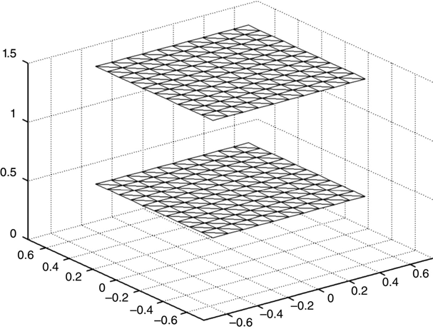
FIGURE 6.8
Triangular cell structure created by mesh_gen_1.
An important attribute of MoM structures is that “what happens in mesh_gen_1 stays in mesh_gen_1.” The all_tris array has node location and voltage information organized by triangles, but there is no numbering of nodes. This means that different geometric structures may share common node locations, but the MoM analysis doesn’t know whether these are common node locations or just very close node locations. A possible problem here is that it also doesn’t know whether, say, two planes at different voltages are touching or even crossing through each other. Since we are concerned more with the MoM analysis than with the grid creation subtleties, we shall leave this type of checking to visual inspection.
The mesh_gen_1 program uses different colors to represent the voltage of the different electrodes. This is, of course, not possible in a black-and-white publication. Two lines that suppress the color information are shown in the listing.
Once the all_tris array has been defined, mom_tri_2 is identical to mom_tri_1. The resulting calculation predicts a capacitance of 29.8 pF.
The MATLAB tic-toc timer function shows that virtually all of the execution time in this program is used by the get_L_1 function. The L array is of size (number of right triangles).2 The number of elements in this array increases quickly according to the number of triangles in the structure. L is a fully populated array. The get_L_1 function addresses every element of this array using a pair of nested loops. While writing get_L_1 this way shows what the function is doing clearly, it does not fully utilize MATLAB’s efficiency in processing vectorized (no explicit) loops.
The get_L_2 function is a direct replacement for get_L_1, but with no explicit loops. It could probably be written to operate more efficiently than it does, but the code was generated to parallel get_L_1 as closely as possible. Here is the get_L2_.m program — a vectorized version of get_L_1.m:
function [L] = get_L_2(rt_tris)
% Generate the L array from the right triangles


 eps0 = 8.854;


[n,junk] = size(rt_tris);
 fprintf('Number of right triangles = %d
', n)


 a2 = rt_tris(:,4:6); a1 = rt_tris(:,1:3);
 a_vec_sq = sum((a2 - a1)'.^2); a_vec = sqrt(a_vec_sq);
 b2 = rt_tris(:,7:9); b1 = rt_tris(:,1:3);
 b_vec_sq = sum((b2 - b1)'.^2); b_vec = sqrt(b_vec_sq);
 c2 = rt_tris(:,7:9); c1 = rt_tris(:,4:6);
 c_vec_sq = sum((c2 - c1)'.^2); c_vec = sqrt(c_vec_sq);
 scl_vec = (a_vec + b_vec)/4;
 err_vec = (a_vec_sq + b_vec_sq - c_vec_sq)./(a_vec_sq + b_vec_sq);
 err_max = max(abs(err_vec));
 fprintf ('Right triangle err_max = %g
', err_max)
 bary = (rt_tris(:,1:3) + rt_tris(:,4:6) + rt_tris(:,7:9))/3;


 th1_vec = -atan(b_vec./2./a_vec); %-atan2(b,2*a);
 th2_vec = pi - atan(2.*b_vec./a_vec); %pi - atan2(2*b,a);
 th3_vec = 3*pi/2 - atan(b_vec./a_vec); %3*pi/2 - atan2(b,a);


 t1_vec = b_vec/3./sqrt(1 + b_vec.^2./a_vec.^2).*log(tan(.5*(th2_vec …
   + atan(b_vec./a_vec)))./tan(.5*(th1_vec + atan(b_vec./a_vec))) );
 t2_vec = -a_vec/3.*log(tan(th3_vec./2 + pi/4.)./tan(th2_vec./2 + pi/4.));
 t3_vec = -b_vec/3.*log(tan(th1_vec./2)./tan(th3_vec./2));


 L_self_vec = (t1_vec + t2_vec + t3_vec)./(2*pi*eps0.*a_vec.*b_vec);


 bx = bary(:,1); xs = (repmat(bx,1,n) - repmat(bx',n,1)).^2;
 by = bary(:,2); ys = (repmat(by,1,n) - repmat(by',n,1)).^2;
 bz = bary(:,3); zs = (repmat(bz,1,n) - repmat(bz',n,1)).^2;
 r = sqrt(xs + ys + zs);
 a_mat = repmat(a_vec',1,n);
 b_mat = repmat(b_vec',1,n);
 L_self_mat = repmat(L_self_vec',1,n);
 scl_mat = repmat(scl_vec',1,n);
 L = 1./(4*pi*eps0*r + 1./L_self_mat./(1 + r./scl_mat));


end
To switch to the vectorized function, triangles_1.m merely replaces the line
with
Since the calculations are identical, the results will be identical. The execution time should decrease by approximately a factor of 150.
6.7 Calculating Voltages
Before proceeding to some more interesting geometries, let’s consider the issue of finding the voltage and the electric field at arbitrary points in space, particularly near our structure. Returning to our basic definitions, we have
where λ
i,j
is the voltage at point j due to all of the (charged) rectangles with barycenters (xj
,yj
,zj
). The notation λ
is used to differentiate this term from the Li,j
term that was used to calculate q. The methods for calculating the two terms are similar; the i in Li,j
refers to the contribution to the voltage at the barycenter of the ith triangle due to the charge on the jth triangle, and the i in λ
i,j
refers to the contribution to the voltage at field point i due to the charge on the jth triangle. In the former case we had set the voltage on all triangles to their applied (boundary) values and found the charge distribution qj
, which supports these applied values. In the latter case we will use the charge distribution qj
, which we have used to find the voltage at an arbitrary point i. If i happens to be the barycenter of one of the electrode triangles, the voltage we find should be the original applied voltage (boundary condition) for that triangle. Here is the get_V.m program—a function used to calculate voltage at an arbitrary point:
function V = get_V(pt,rt_tris,q)
% Get voltage at a given point
% This is actually a reduced version of get_L_2


 xi = pt(1); yi = pt(2); zi = pt(3);


 eps0 = 8.854;


 a2 = rt_tris(:,4:6); a1 = rt_tris(:,1:3);
 a_vec_sq = sum((a2 - a1)'.^2); a_vec = sqrt(a_vec_sq);
 b2 = rt_tris(:,7:9); b1 = rt_tris(:,1:3);
 b_vec_sq = sum((b2 - b1)'.^2); b_vec = sqrt(b_vec_sq);
 c2 = rt_tris(:,7:9); c1 = rt_tris(:,4:6);
 c_vec_sq = sum((c2 - c1)'.^2); c_vec = sqrt(c_vec_sq);
 scl_vec = (a_vec + b_vec)/4;
 bary = (a1 + a2 + b2)/3;


 th1_vec = -atan(b_vec./2./a_vec);
 th2_vec = pi - atan(2.*b_vec./a_vec);
 th3_vec = 3*pi/2 - atan(b_vec./a_vec);


 t1_vec = b_vec/3./sqrt(1 + b_vec.^2./a_vec.^2).*log(tan(.5*(th2_vec …
   + atan(b_vec./a_vec)))./tan(.5*(th1_vec + atan(b_vec./a_vec))) );
 t2_vec = -a_vec/3.*log(tan(th3_vec./2 + pi/4.)./tan(th2_vec./2 + pi/4.));
 t3_vec = -b_vec/3.*log(tan(th1_vec./2)./tan(th3_vec./2));


 L_self_vec = (t1_vec + t2_vec + t3_vec)./(2*pi*eps0.*a_vec.*b_vec);


 r_vec = [xi - bary(:,1), yi - bary(:,2), zi - bary(:,3)];
 r = sqrt(r_vec(:,1).^2 + r_vec(:,2).^2 + r_vec(:,3).^2);
 L = 1./(4*pi*eps0*r + 1./L_self_vec'./(1 + r./scl_vec'));


 V = sum(q.*L);


end
A call to get_V specifying the point of interest as a 1×3 vector [xi
,yi
,zi
], along with the rt_tris and q arrays, returns the value of V at that point. Figure 6.9 shows the results of calculating voltage as a function of x at y = 0 for several values of z.
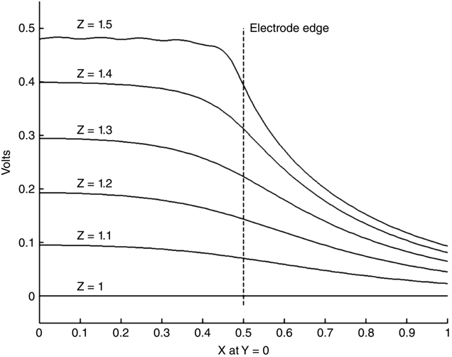
FIGURE 6.9
Voltage profiles of mom_tri_2.m example.
Almost everything in Figure 6.9 is what would be expected. The potential at x = 0 increases linearly with z from v = 0 at z = 0.5 to v = 0.5 at z = 1.5 The voltage equipotentials are parallel to the electrodes most of the way to the end of the electrodes, beginning to fall as they approach (being under the) electrode edge, and then falling toward 0 with increasing x. The farther the equipotential is from the electrode (decreasing z in this figure), the less control the electrode has on the shape of the equipotential as the edge is approached.
On closer inspection we can see that the z = 1.5 equipotential line isn’t quite right. First, the equipotential is at ~ 0.48 V, not the 0.5 V set by the electrode voltage. Also, there is an undulation in the line itself. The problem here is that we are too close to the charged triangles and the λ approximation [equation (6.20), as used in get_V.m] is not that accurate. To do the job better, we would need a get_V function that actually integrates (numerically) over all the charged triangles. A significant weakness in the λ approximation is that it ignores the orientations of the charged triangles — only the barycenter locations are considered. While a function for calculating L that does the job properly would run very slowly, due to the size of the job, a function for calculating λ would be a reasonable undertaking; remember that, to calculate λ, we need (number of triangles) integrations, while to calculate L, we need the square of this amount.
6.8 Calculating the Electric Field
The empirical relationships used in the L and λ approximations of the previous sections were easy to create. All we had to do was find a smooth function (with the approximately correct shape) that connected the two asymptotic regions, the simple V ~ q/r relationship for large ri,j and the known V function (the L self term) at r = 0.
The L self term resulted from the integration of
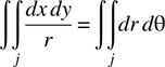
where region j is the area of the triangle (or rectangle) under consideration and includes the point r = 0. While the details of the integration can be very involved, depending upon the shape of the region, this integral always exists.
On the other hand, finding the (magnitude of the) electric field at the barycenter of a uniformly charged planar region requires calculating the integral

where once again, r = 0 is in the integration region. Since
any integration with r = 0 as one of the limits does not exist.
In other words, there is no electric field equation analog to the self L term. The electric field goes to zero at the barycenter of a uniformly charged region. We must look elsewhere for a simple estimate of the electric field. We could, of course, perform the (numerical) integrations of the charged regions, but this approach carries the same caveats as those discussed in Section 6.7 for approximating V.
A simple but in most cases effective approximation is to use a centered numerical derivative, such as
where δ is small enough to allow for the desired resolution, but large enough so as to avoid numerical roundoff errors in the calculations.
Setting δ = 0.01, Figure 6.10 is a repeat of Figure 6.9 except that now the z component of the electric field (Ez ) is plotted. The average electric field between two plates 1 m apart with 1 V difference between them is, of course, 1 V/m. For z = 1.0 through z = 1.4, we see this at x = 0, within a few percent. As we increase x, for z = 1.0 through z = 1.2 the field falls off as x nears the electrode edge, then falls toward 0 with increasing x. For z = 1.3 and particularly at z = 1.4, the electric field begins to peak near the electrode edge, a consequence of the charge density concentration at the electrode edges.

FIGURE 6.10
Ez
profiles of mom_tri_2.m example.
At z = 1.5 we see a very nonphysical situation. Figure 6.10 shows an essentially constant Ez of -0.2 V/m. How could the same calculation that gave such reasonable results for the other values of z perform so badly here?
The answer to this puzzle is that the program is calculating—as computer programs almost always do—exactly what we programmed it to calculate. Equation (6.24) prescribes a centered derivative (with respect to z) calculation about the chosen point. Since our electrode in this example has 0 thickness, the program is subtracting a voltage below the electrode from a voltage above the electrode.
Figure 6.11 is a closeup view of Figure 6.10, with z values between 1.4 and 1.5. There is a range of results going from the nonsensical value at z = 1.50 to the reasonable value at z = 1.40. Of interest is that in this model, a = b = 0.1 for all of the triangles. While not an actual calculation, the size of the triangles involved provides a good rule of thumb as to how useful calculations of V and E can be: If you are farther away from an electrode than the larger of a and b for one of the larger triangles in the region, then the values of V and E will be reasonable. If not, anything can happen.
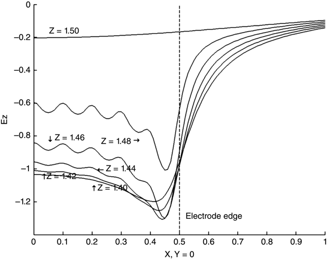
FIGURE 6.11
Ez
profiles of mom_tri_2.m example, z near top electrode.
6.9 Three-Dimensional Structures
There are an infinite number of possible structures that can be described and analyzed. The limiting factors are the needs of the user and the sophistication of the meshing package being used. In this section we’ll examine a few examples to show the possibilities and some of the issues that arise. The first example is shown in Figure 6.12.
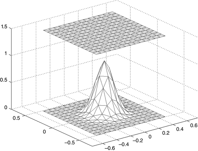
FIGURE 6.12 Parallel plate with a Gaussian “lump” on one plate.
This meshing is accomplished by changing just two lines in mesh_gen_1.m:
- Change h = 1.0; to h = 1.5; for the top electrode.
- On line 31, change z = z + h; to z = exp(-(7*x).^2 – (7*y).^2);.
Note that this change is transparent to the calling program mom_tri_2.m. As long as the data file is in the correct format, mom_tri_2.m will process the data, calculate the charge on each triangle’s barycenter, and calculate the capacitance.
The tip of the Gaussian curve in Figure 6.12 doesn't look particularly Gaussian; the resolution is too low in this region. There are numerous ways to improve this situation. Resolution everywhere could be improved, and the tip of the curve would benefit from this improvement. This solution is always possible but rarely desirable because the number of cells grows quickly, and the number of Li,j matrix elements to calculate grows with the square of the number of cells. Extra nodes could be added manually, but this is a time-consuming and usually haphazard process.
The two lines labeled “improved tip resolution” in mesh_gen_1.m handle this situation by recalculating the grid spacing of the lower conductor. Instead of a linear spacing (such as used in the upper conductor), all of the points are moved closer to x = 0, y = 0. This results in the greatly improved shape of the tip, shown in Figure 6.13.
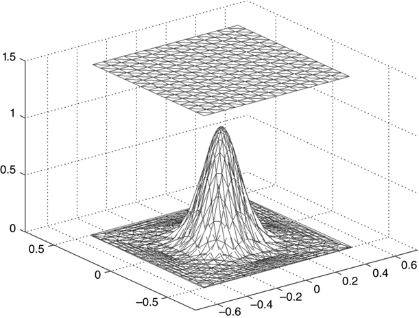
FIGURE 6.13 Structure shown in Figure 6.12 with increased resolution of Gaussian tip.
The freely available distmesh package4 creates meshings using MATLAB code that add greatly to our capabilities.5 This package comes with extensive documentation and examples that won't be repeated here. We will, however, use two distmesh examples as mesh sources for our own examples. Consider the following program, distmesh_example.m—a distmesh code for a square plate with a circular hole:
% distmesh example code


fd = @ (p) ddiff (drectangle(p,-1,1,-1,1), dcircle(p,0,0,0.5));
fh = @ (p) 0.05 + 0.3*dcircle(p,0,0,0.5);
[p,t] = distmesh2d(fd,fh,0.05,[-1 -1; 1 1], [-1 -1; -1, 1; 1,-1; 1,1]);
The three lines of MATLAB code shown produce the sophisticated zoning of Figure 6.14.This simple distmesh code has created (the meshing for) a rectangular electrode with a hole in the center. The distmesh code also produces output arrays that are easily translatable to the all_tris array format used by the examples in this book.
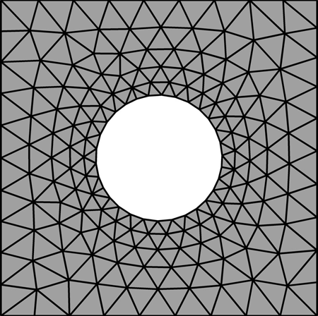
FIGURE 6.14 Results of the distmesh sample code distmesh_example.m.
The easiest way to show how to convert distmesh output to the all_tris format is with an example. The MATLAB function mesh_gen_3.m combines the distmesh example (displayed above) with the Gaussian post example shown previously and generates the graphics to display the result. Here is the program mesh_gen_3.m—a structure built by combining previous examples:
function all_tris = mesh_gen_3
% mesh_gen_3.m 3d figures generated w/distmesh and Matlab
%  this is the emitter region of a Spindt Tip structure


 figure(1)
 fd = @ (p) ddiff (drectangle(p,-1,1,-1,1), dcircle(p,0,0,0.5));
 fh = @ (p) 0.05 + 0.3*dcircle(p,0,0,0.5);
 [p,t] = distmesh2d(fd,fh,0.05,[-1 -1; 1 1], [-1 -1; -1, 1; 1,-1; 1,1]);


 figure(2)
 X = p(:,1);
 Y = p(:,2);
 Z = ones(length(X),1);
 trimesh(t,X,Y,Z);
 hold on
 C = [.5,.5,.5; .5,.5,.5; .5,.5,.5];
 colormap(C);


 all_tris = [];
 nr_tris = length(X);   %%
 for i = 1:nr_tris
  n1 = [X(t(i,1)), Y(t(i,1)), Z(t(i,1))];
  n2 = [X(t(i,2)), Y(t(i,2)), Z(t(i,2))];
  n3 = [X(t(i,3)), Y(t(i,3)), Z(t(i,3))];
  all_tris = [all_tris;[n1,n2,n3], .5];
 end
 % ----------------------------------


 X = p(:,1);
 Y = p(:,2);
 Z = .98*ones(length(X),1);
 trimesh(t,X,Y,Z);
 nr_tris = length(X);   %%
 for i = 1:nr_tris
  n1 = [X(t(i,1)), Y(t(i,1)), Z(t(i,1))];
  n2 = [X(t(i,2)), Y(t(i,2)), Z(t(i,2))];
  n3 = [X(t(i,3)), Y(t(i,3)), Z(t(i,3))];
  all_tris = [all_tris;[n1,n2,n3], .5];
 end


 % ----------------------------------------------------


 % Gaussian post, compress grid spacing near the center
 test = [-1.2 : .14 : 1.2];
 [x,y] = meshgrid(test);
 rad = sqrt(x.^2 + y.^2);
 x = x.*rad/2; y = y.*rad/2;
 tri = delaunay(x,y);


 z = exp(-(7*x).^2 - (7*y).^2);
 tr = TriRep(tri, x(:), y(:), z(:));
 trimesh(tr);


 nodes = tr.X;
 cons = tr.Triangulation;
 [nr_tris,p] = size(cons);
 for i = 1:nr_tris
   all_tris = [all_tris;[nodes(cons(i,1),:), nodes(cons(i,2),:), …
      nodes(cons(i,3),:), -.5]];
 end


 axis ([-1.5 1.5 -1.5 1.5 0. 1.2])


end
There are actually two stacked identical distmesh structures in this example. The upper electrode has effectively been given some thickness. If an even thicker electrode were desired, in addition to separating the two identical layers, more sidewall layers would have to be added.
The simple script mom_tri_3.m calls mesh_gen_3 to generate the electrode meshes (see Figure 6.15), triangles_1 to find the charge on the electrodes, and then get_V to examine a voltage profile.
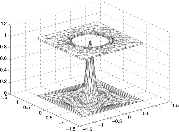
FIGURE 6.15
Combined electrode structure created by mesh_gen_3.
The program mom_tri_3.m—a calling script for mesh_gen_3 structures—is as follows:
% mom_tri_3.m script for handling triangular cell mom problems


close all; clear


all_tris = mesh_gen_3;


[q, rt_tris] = triangles_1(all_tris);


q = q(1:end-1);
C1 = sum(q.*(q > 0))


% look at a voltage profile


figure(3)
x_plot = [-.8 : 0.002 : .8]; V = [];


for i = 1 : length(x_plot)
 pt = [0,x_plot(i), .99];
 V = [V, get_V(pt,rt_tris,q)];
end
plot(x_plot, V)
axis ([-.8 .8 -.6 .6])
xlabel ('X at Y = 0, Z = 0.99')
ylabel ('Voltage')
In mesh_gen_3, the two (identical) planar electrode layers are at z = 1.00 and z = 0.98, both at the same potential (0.5 V) (see Figure 6.16). The Gaussian post structure peaks at z = 1.00, it is at -0.5 V. The voltage profile is taken as a function of x at y = 0, z = 0.99. This profile starts and ends at the (x) edges of the hole in the upper layers, at a z value midway between them. It passes directly through the tip of the Gaussian post, 0.01 below the peak of the tip.
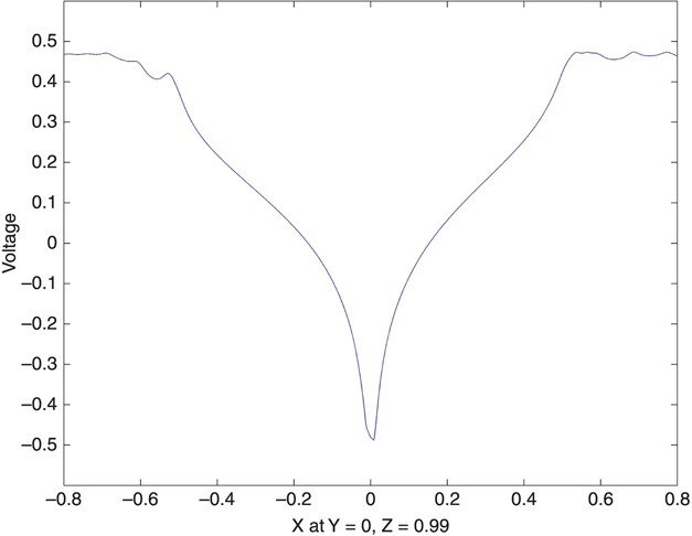
FIGURE 6.16
Voltage profile for mesh_gen_3 structure.
Figure 6.17 shows two concentric spheres. This structure was generated using distmesh, as shown in MATLAB function mesh_gen_4.m.

FIGURE 6.17 Two concentric spheres, radii 1 and 2.
Here is program mesh_gen_4.m—a function that can be used to generate concentric sphere meshing:
function all_tris = mesh_gen_4
% mesh_gen_4.m 3d figures generated w/distmesh
%  These are concentric spheres, r = 1 and r = 2


 figure(2)
 all_tris = [];
 C = [.5,.5,.5; .5,.5,.5; .5,.5,.5];
 colormap(C);


 % ------ outer sphere -----------------------


 fd = @ (p) dsphere(p,0, 0, 0, 2);
 [p,t] = distmeshsurface(fd, @huniform, 0.4, 1.1*[-2 -2 -2; 2 2 2]);


 X = p(:,1);
 Y = p(:,2);
 Z = p(:,3);
 trimesh(t,X,Y,Z);
 hold on
 nr_tris = length(t);
 for i = 1:nr_tris
  n1 = [X(t(i,1)), Y(t(i,1)), Z(t(i,1))];
  n2 = [X(t(i,2)), Y(t(i,2)), Z(t(i,2))];
  n3 = [X(t(i,3)), Y(t(i,3)), Z(t(i,3))];
  all_tris = [all_tris;[n1,n2,n3], .5];
 end


% -- inner sphere -----------------------------------------


 figure(3)
 fd = @ (p) dsphere(p,0,0,0, 1);
 [p,t] = distmeshsurface(fd, @huniform, 0.2, 1.1*[-1 -1 -1; 1 1 1]);
 close 3


 X = p(:,1);
 Y = p(:,2);
 Z = p(:,3);
 figure(2)
 trimesh(t,X,Y,Z);


 nr_tris = length(t);
 for i = 1:nr_tris
  n1 = [X(t(i,1)), Y(t(i,1)), Z(t(i,1))];
  n2 = [X(t(i,2)), Y(t(i,2)), Z(t(i,2))];
  n3 = [X(t(i,3)), Y(t(i,3)), Z(t(i,3))];
  all_tris = [all_tris;[n1,n2,n3], -.5];
 end


 axis ([-3 3 -.5 3–3 3])
end
Figure 6.17 shows the outer sphere partially cut away so as to expose the inner sphere (see line 50 in mesh_gen_4).
MATLAB script mom_tri_4 calculates the capacitance of this structure and produces the curve of the voltage versus the radius between the spheres. Because the electric field in this structure is confined to the region between the spheres, an offset voltage is required to correct for the voltage at infinity—the outside world sees only the outer sphere. This voltage is automatically calculated as q (end) by mom_tri_4 and must be added to the voltage predicted (lines 8 and 22 in mom_tri_4) to get the correct results.
The mom_tri_4 function predicts a capacitance of 227.2 pF. From basic considerations, where a and b are the inner and outer radii, respectively, we obtain

From which
The model’s prediction is 2% above the exact answer.
The voltage between the spheres is only a function of r (symmetry demands this) and again, from basic considerations [a direct extension of equation (6.25)], we obtain

The program mom_tri_4.m—the script used to model concentric spheres—is as follows:
% mom_tri_4.m script for handling triangular cell mom problems


close all; clear


all_tris = mesh_gen_4;
[q, rt_tris] = triangles_1(all_tris);


V_off = q(end)
q = q(1:end-1);
C1 = sum(q.*(q > 0))


% look at a voltage profile


figure(4)
x_plot = [1. : .05 : 2]; V = []; V_exact = [];


for i = 1 : length(x_plot)
 pt = [x_plot(i), 0, 0];
 V = [V, get_V(pt,rt_tris,q)];
 V_exact = [V_exact, -.5 - 2*(1/x_plot(i) - 1)];
end
plot(x_plot, V + V_off, 'kx', x_plot, V_exact, 'k')
xlabel ('X at Y = 0, Z = 0')
ylabel ('Voltage')
The mom_tri_4.m program plots the comparison of the model results and the analytic voltage between the spheres. The result is shown in Figure 6.18. For the most part the results of the model (the x values) agree very well with the analytic expression (the continuous line).
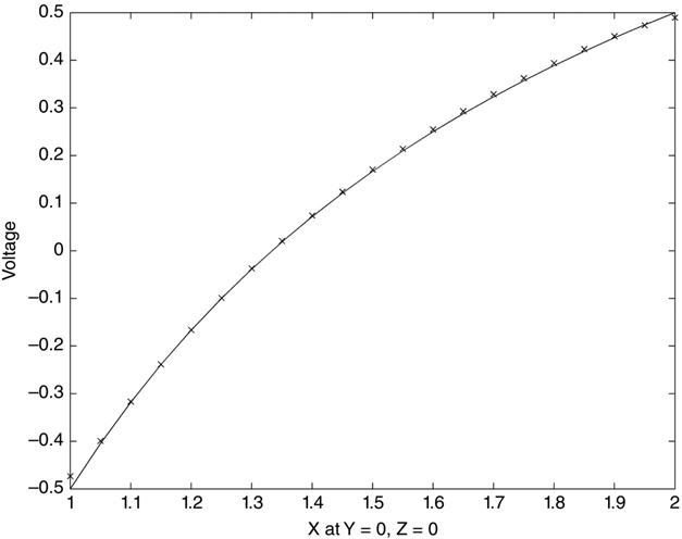
FIGURE 6.18 V(r) between the spheres: model and analytic results.
There is some small degree of error at both spheres (the left and right extremes of the figure), as there was in previous structure voltage scans. Again, the error arise when we try to “get too close” to an electrode.
6.10 Charge Profiles
In previous sections, when electrodes were rectangular and consisted of square cells, it was easy to examine a charge profile. In the more general case of arbitrarily sized and placed triangular cells, unfortunately, this is not the case.
MATLAB program mom_tri_5.m creates a worst-case situation to illustrate the issues:
- Program
mom_tri_5.m—MATLAB script used to generate random node points in a square region:% mom_tri_5.m script for looking at a charge profile close all; clear % note that mesh_get_5 uses a random number generator, results won't repeat all_tris = mesh_gen_5; [q, rt_tris] = triangles_1(all_tris); V_off = q(end) q = q(1:end-1); C1 = sum(q.*(q > 0)) % get some barycenters and areas for all the rt_tris [barys, areas] = process(rt_tris); tol = .02; % find all triangles with |y| of barycenter < tol n = length(q); x_used = []; rho_used = []; for i = 1: n if abs(barys(i,2)) < tol if q(i) > 0 x_used = [x_used, barys(i,1)]; rho_used = [rho_used, q(i)/areas(i)]; end end end figure(2) plot(x_used, rho_used, 'x') xlabel ('x at y = 0, top electrode') ylabel ('charge density') - Program
mesh_gen_5.m:function all_tris = mesh_gen_5 % mesh_gen_5.m %figure(1) %hold on %C = [.5,.5,.5; .5,.5,.5; .5,.5,.5]; %colormap(C); all_tris = []; x = -.5 + rand(400,1); y = -.5 + rand(400,1); tri = delaunay(x,y); z = ones(size(x)); tr = TriRep(tri, x(:), y(:), z(:)); trimesh(tr); hold on C = [.5,.5,.5; .5,.5,.5; .5,.5,.5]; colormap(C); nodes = tr.X; cons = tr.Triangulation; [nr_tris,p] = size(cons); for i = 1:nr_tris all_tris = [all_tris;[nodes(cons(i,1),:), nodes(cons(i,2),:), … nodes(cons(i,3),:), .5]]; end % ---------------------------------------------------- % flat electrode test = [-.5 : 0.05 : .5]; [x,y] = meshgrid(test); tri = delaunay(x,y); z = zeros(size(x)); tr = TriRep(tri, x(:), y(:), z(:)); trimesh(tr); nodes = tr.X; cons = tr.Triangulation; [nr_tris,p] = size(cons); for i = 1:nr_tris all_tris = [all_tris;[nodes(cons(i,1),:), nodes(cons(i,2),:), … nodes(cons(i,3),:), -.5]]; end axis ([-.7 .7 -.7 .7 -.2 1.2]) end - Program
process.m:function [barys, areas] = process(rt_tris) % %n = max(size(used_tris) %fprintf('Number of used right triangles = %d ', n) a2 = rt_tris(:,4:6); a1 = rt_tris(:,1:3); a_vec_sq = sum((a2 - a1)'.^2); a_vec = sqrt(a_vec_sq); b2 = rt_tris(:,7:9); b1 = rt_tris(:,1:3); b_vec_sq = sum((b2 - b1)'.^2); b_vec = sqrt(b_vec_sq); barys = (rt_tris(:,1:3) + rt_tris(:,4:6) + rt_tris(:,7:9))/3; areas = (a_vec.*b_vec/2)'; end
Then mom_tri_5.m, using the function mesh_gen_5.m, creates a new square electrode parallel plate capacitor (see Figure 6.19). One of the electrodes is identical to the previously generated simple square electrode with triangular cells. The other electrode, however, is created using a set of points randomly scattered about the square electrode region.
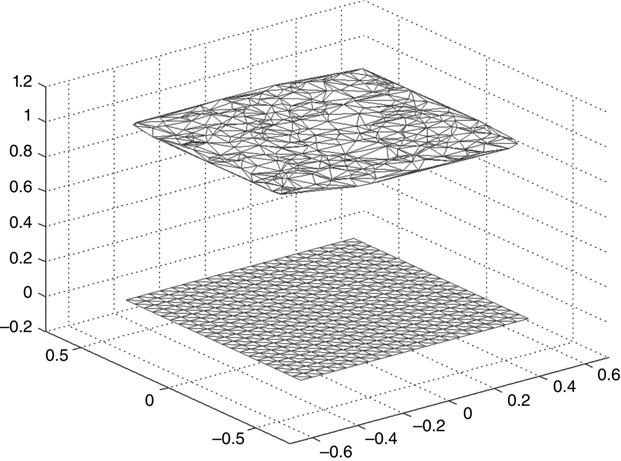
FIGURE 6.19 Parallel plate capacitor with one electrode composed of randomly generated cells.
Remember that this program will not repeat exactly; not only will your results not duplicate the results shown, they won't be the same twice.
The random cell electrode looks enough like a square electrode that the capacitance calculation repeats fairly well. Suppose, however, that we want to calculate a charge density profile. For this example, we choose the charge density as a function of X at Y = 0 along the upper electrode.
The issues in performing this calculation start surfacing immediately. Not only are all the triangles different from each other; their vertices, and therefore their barycenters, are also random distributions.
One way to proceed is to select the triangles whose barycenters are within some small distance of y = 0 and use these barycenters “as if” they are at y = 0. Figure 6.20 shows the result of this calculation.
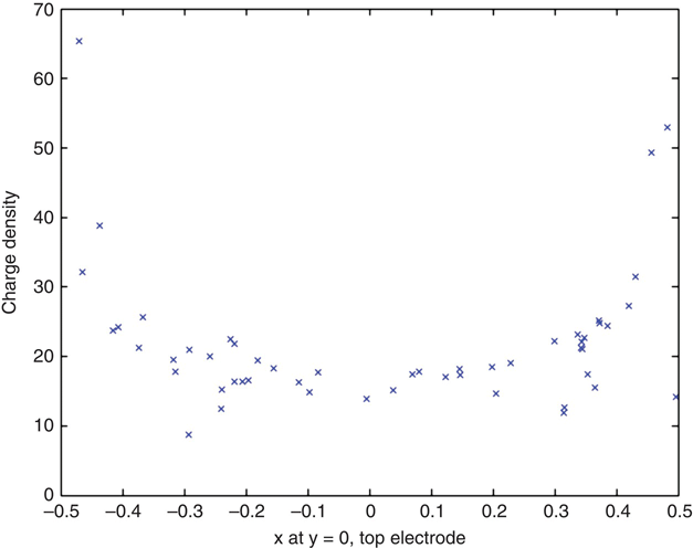
FIGURE 6.20 Charge density versus X at Y = 0 approximated by using triangles with |Y| < 0.02.
When all the cells in an electrode were identical squares, the charge profile using appropriate q values gave us the correct distribution curve. Since the triangles’ areas are all different in this situation, it is necessary to divide each value of q by the area of its triangle to obtain a charge density value.
Figure 6.20 is a reasonable but not excellent portrait of the charge distribution in question. It could be improved by fitting the data to a polynomial and discarding outliers. Alternatively, the charge density in several cells with barycenters close to each data point’s x value could be fit to a polynomial and then the value at (x,y = 0) determined. There is no ideal way to resolve this issue.
Voltage and electric field values in this example will be reasonable far away from the electrode(s). Values near the electrodes will be more erratic than in previous examples because the charge distribution itself is more erratic.
Problems
Two preliminary notes are useful here:
- There is almost never only one way to code an algorithm to achieve a particular task. For creation of node layouts for mesh generation, there is similarly almost never only one good solution. The listings shown below are examples that work; nothing more is claimed for them.
- In the example solutions to follow, the color mapping is left at the MATLAB default and the option to change it to black-and-white format is shown commented out. For more complicated structures (and for a data-file-driven package), a more inventive use of the available color mapping would be very valuable.
6.1 Create a version of mesh_gen, called by mom_tri_2, that creates a parallel-plate structure with circular electrodes.
6.2 Upgrade the results of Problem 6.1 to allow the creation of washers, namely, circular disks containing centered holes.
6.3 Upgrade the results of Problem 6.2 so that the washers interlock (in a chain-link configuration).
6.4 Create a mesh_gen function (and possibly supporting functions) to allow for the generation of meshed rectangles parallel to any axis. Use these functions to generate a box-within-a-box structure.
6.5 Create a mesh_gen function to generate spheres. Construct two concentric spheres with radii = 1, 2, and calculate the capacitance between them. Compare this result to the result using the distmesh package.
References
- 1.
http://en.wikipedia.org/wiki/Center_of_mass. - 2. P. Lazic, H. Stefancic, and H. Abraham, The Robin Hood method—a novel numerical method for electrostatic problems based on a non-local charge transfer,
Physics.com-ph(Nov. 20, 2004). - 3.
http://en.wikipedia.org/wiki/Delaunay_triangulation. - 4.
http://persson.berkeley.edu/distmesh/. - 5. P.-O. Persson and G. Strang, A simple mesh generator in MATLAB, SIAM Rev. 46 (2): 329–345 (2004).